Article

Reducing Particle Exposure and SARS-CoV-2 Risk in Built Environments through Accurate Virtual Twins and Computational Fluid Dynamics

1
Dassault Systemes SIMULIA Meitnerstraße 8, 70563 Stuttgart, Germany
2
Institut für Energie-und Umwelttechnik (IUTA) e.V., 47229 Duisburg, Germany
*
Authors to whom correspondence should be addressed.
Atmosphere 2022, 13(12), 2032; https://doi.org/10.3390/atmos13122032
Submission received: 16 September 2022 / Revised: 24 November 2022 / Accepted: 29 November 2022 / Published: 3 December 2022

Abstract

:
The World Health Organization has pointed out that airborne transmission via aerosol particles can be a strong vector for the spread of SARS-CoV-2. Protecting occupants from infectious diseases or harmful particulate matter (PM) in general can be challenging. While experimentally outlining the detailed flow of PM in rooms may require complex setups, computational fluid dynamics (CFD) simulations can provide insights into improving the safety of the built environment and the most effective positioning of air-purifying devices. While previous studies have typically leveraged Reynolds-averaged Navier–Stokes (RANS) approaches for predicting particle propagation, the turbulence length scales accurately captured in these simulations may not be sufficient to provide a realistic spread and the mixing of particles under the effects of forced convection. In this paper, we experimentally validate a Lattice Boltzmann very large eddy simulation (VLES) approach including particle modeling. We also demonstrate how this simulation approach can be used to improve the effectiveness of air filtration devices in realistic office environments.

1. Introduction

The modes of transmissions for SARS-CoV-2 can be separated in transmission through direct contact and airborne transmission [1]. While transmission through contact has been the focus of the World Health Organization (WHO) in the early days of the pandemic, later scientific information has justified additional measures focusing on limiting airborne transmission [2]. The latter is of particular concern in confined spaces, where the lack of ventilation and air renewal can help small concentrations of emitted viruses to become infectious over time [3,4,5].
For SARS-CoV-2, the individual virus particles have sizes between 60 and 140 nm, but they are typically embedded in larger droplets. For normal breathing, these droplets have a typical size between 200 to 400 nm upon exhalation [6]. In this size range, the dispersion of aerosols is fully dependent on the confined environment with the particles moving under the effects of Brownian motion, inertia, gravity, evaporation [7], and of course convection by air flow from ventilation systems or other devices. This motion includes the impact of natural convection effects from heaters, electronics, or solar radiation [8].
While measurements can provide information on a local concentration level over time, for the purpose of ensuring a safe working and living space, they are difficult to implement without disturbing the environment, and do not provide information about the transport mechanisms. Simulations can, however, give a better insight into the distribution of concentration levels with time and provide information on how to improve room arrangements or safety measures for reducing the health hazard of occupants.
In order to provide valuable results, a simulation must be able to track the aerosol concentration over time and include thermodynamic effects, which will influence room air currents. Furthermore, in order to represent realistic aerosol mitigation methods and to evaluate their effectiveness, simulations must also be able to take into account the impact of filtering systems or air purifying devices.
In this paper, we propose a Lattice Boltzmann-based method (LBM) for simulating aerosol dispersion and deposition in a realistic room with and without air filtering devices. The LBM approach is well suited to this type of problem as it is intrinsically transient [9]. Furthermore, this specific implementation of LBM employs very large eddy simulation (VLES) to explicitly capture relevant scales of turbulence, rather than modelling them [10]. A literature research shows that Reynolds-averaged Navier–Stokes (RANS) approaches, where turbulence is fully modelled, are typically chosen for aerosol transport predictions in buildings [11]. This modeling leads to approximations on the mechanisms responsible for the transport and, consequently, to uncertainties [12]. This is especially true in scenarios involving strong forced convection which results in mixing, as is the case when air filtering devices are active [13,14,15].
As part of this paper, we present validation results comparing experimental measurements with simulations that capture the concentration of aerosols in a realistic room over 1 h. Measurements are compared to assess the difference in concentration levels with air filtering devices, either active or inactive. Following the validation, we then show how simulation can be used to improve the arrangement of the room, and the positioning of the filtering devices, with the aim of minimizing the infection risk for occupants.
The additional information available in the simulation provides useful insights into exploring alternative room scenarios and into driving changes to minimize the infection risk to occupants. The ambition of this simulation-led methodology is to provide actionable scientific information, which would enable verifying, altering and refining blanket measures currently implemented across the globe. Furthermore, the methodology can be used to verify which measures are not restrictive enough or even potentially putting occupants at risk.
The simulation methodology is extendable to the internal flow behavior of filtering devices, which allows the use of LBM to effectively position filters within air filtering or heating ventilation and air conditioning (HVAC) devices, to achieve simultaneously aerodynamic performance and filter efficiency, and to potentially extend the maximum life of the filters.

2. Materials and Methods

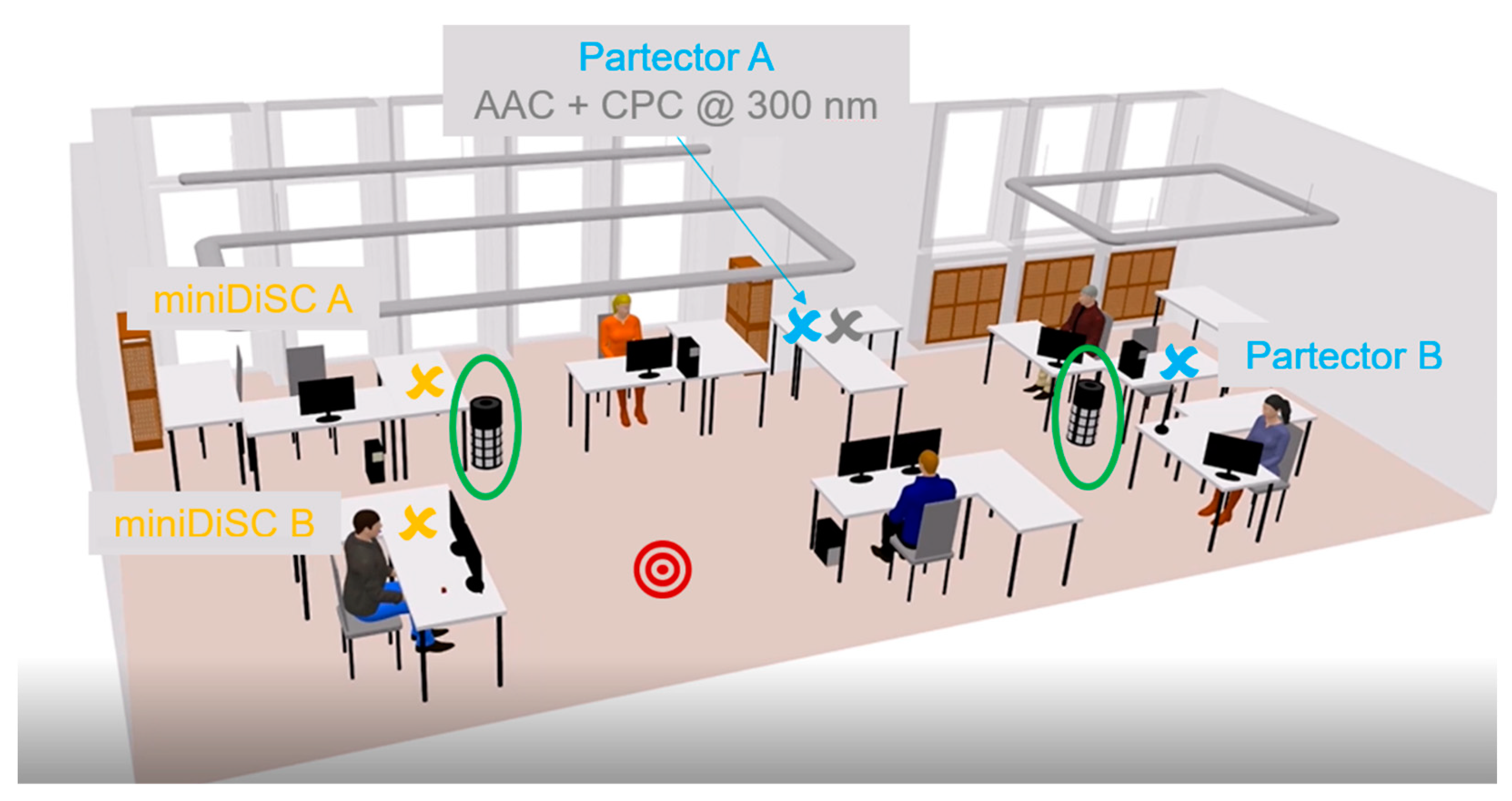
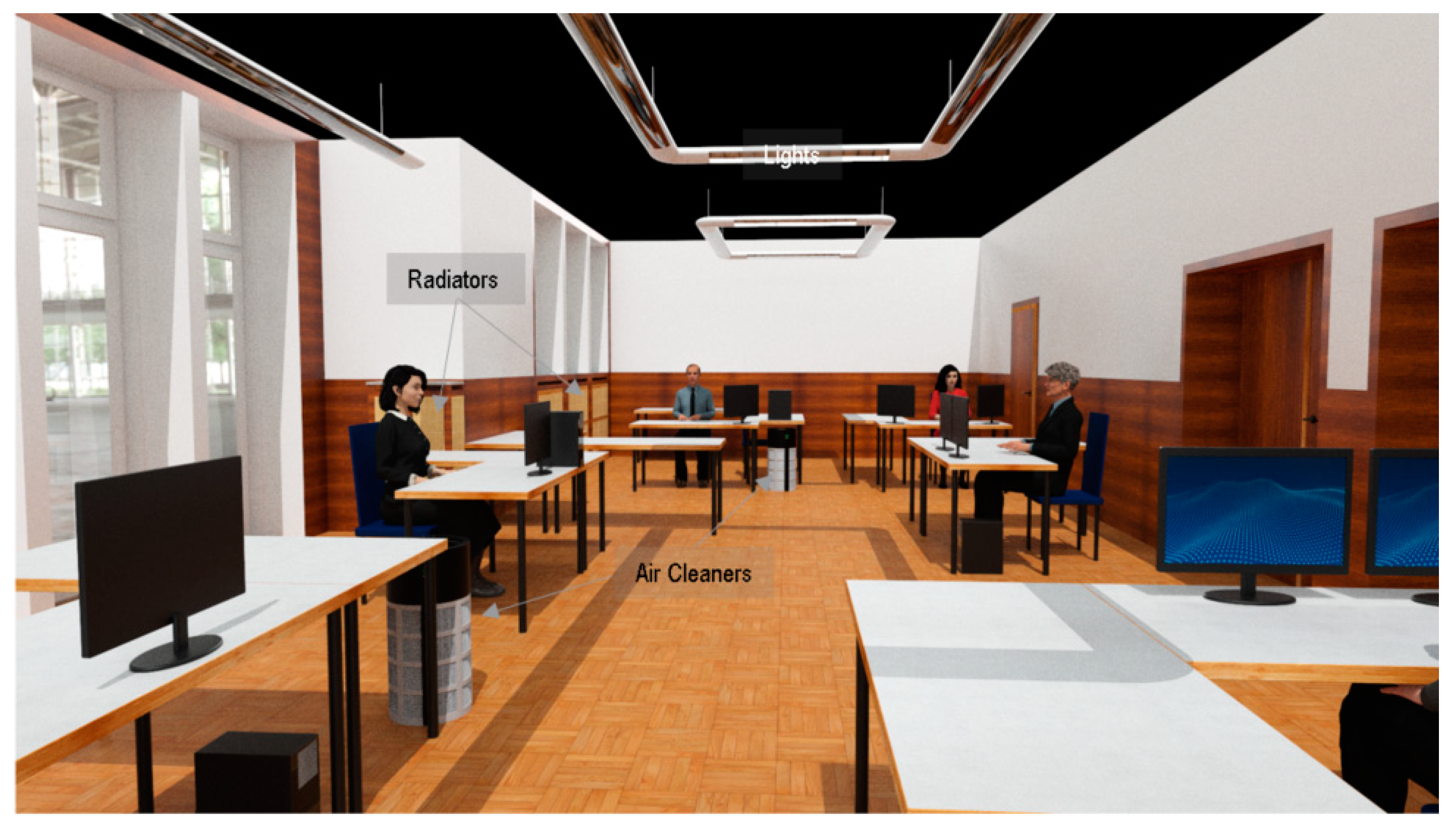
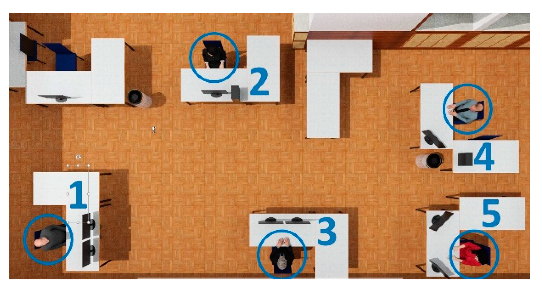
2.1. Experimental Setup

All of the following comparisons between simulation and experiment were conducted in an office room of the Institute for Energy and Environmental Technology (IUTA) e. V. in Duisburg (Germany) in August 2021. The floor area of the room was measured to be 95.5 m2, and the volume 311.3 m3. The room was furnished with several desks, as shown in Figure 1. Four miniaturized measurement instruments were used across the room, consisting of two miniDISC (Fachhochschule Nordwestschweiz; prototype of the later commercialized DiSCmini, Testo GmbH) and two Partector 2 [16]. Both of them measure the total quantity of concentration with reasonable accuracy [17]. As a reference, an aerodynamic aerosol classifier (AAC, Cambustion) was used to classify 300 nm particles, which were then measured with a water-based condensation particle counter (CPC, TSI model 3787). This size is representative for SARS-CoV-2 propagating in fine exhaled droplets. One Partector 2 and the AAC were positioned close to each other in order to calibrate all instruments to the same metric. It should be noted that the particle-measuring devices were directly placed on the table without any stand or offset. It is not known whether a boundary layer developing on the surface of the table could in turn affect the accuracy of the particles measured from this device, with boundary layer sizes expected to be of the order of 1 centimeter in this area [18].
Particles were seeded into the room with an atomizer (model AGK 2000, Palas GmbH), operated with an aqueous 150 g/L NaCl solution at different inlet pressures. The solution droplets, dispersed by the atomizer, were dried by dilution with dry and clean compressed air. Particles were spread across the room by using a desk-mounted fan, in order to achieve a homogenous distribution of particles. Two air cleaners were also installed in the room, with a nominal clean air delivery rate (CADR) of 550 m3/h each. This corresponds to approximately 3.5 air changes per hour (ACH) for this room size. While the virtual twin shows a typical office occupancy, the experiment and simulation validations were conducted at night, with no occupants in the room. All gaps around doors, windows and heating, ventilation and air conditioning (HVAC) unit inlet and outlets were sealed completely, with the result that no airflow could enter or exit the room.

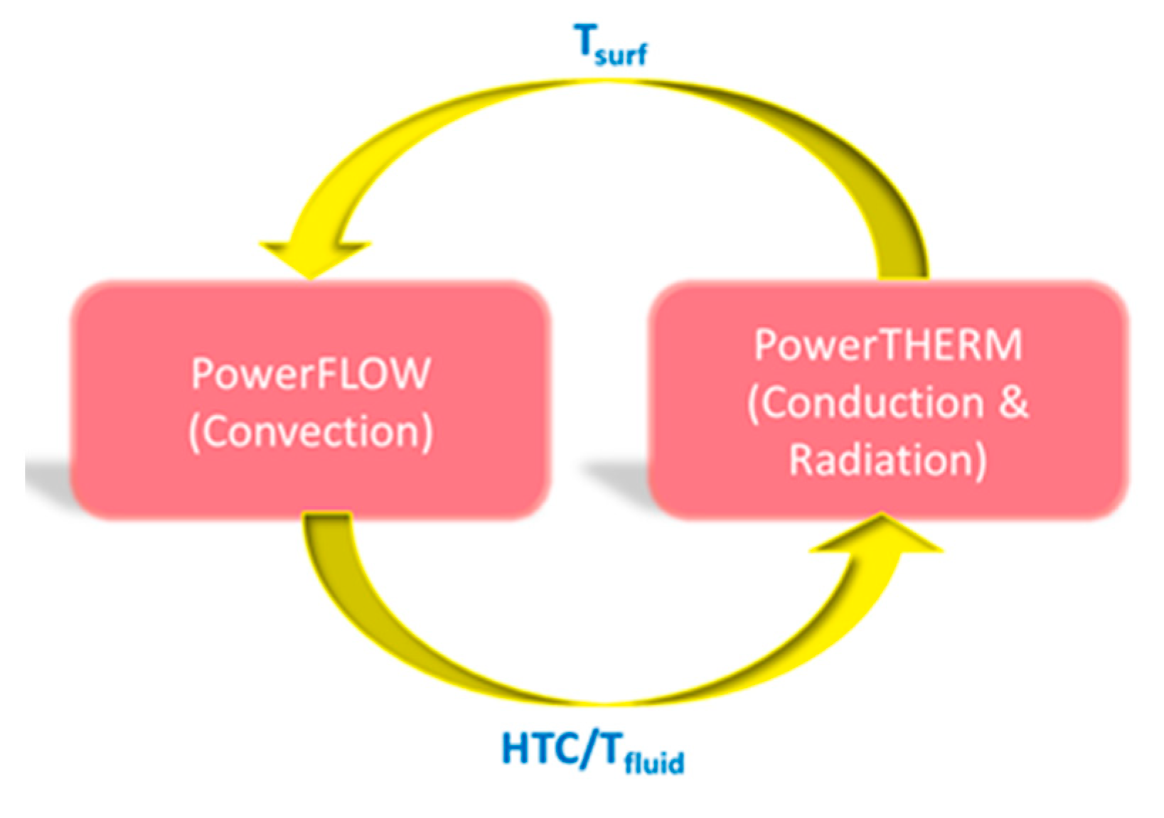
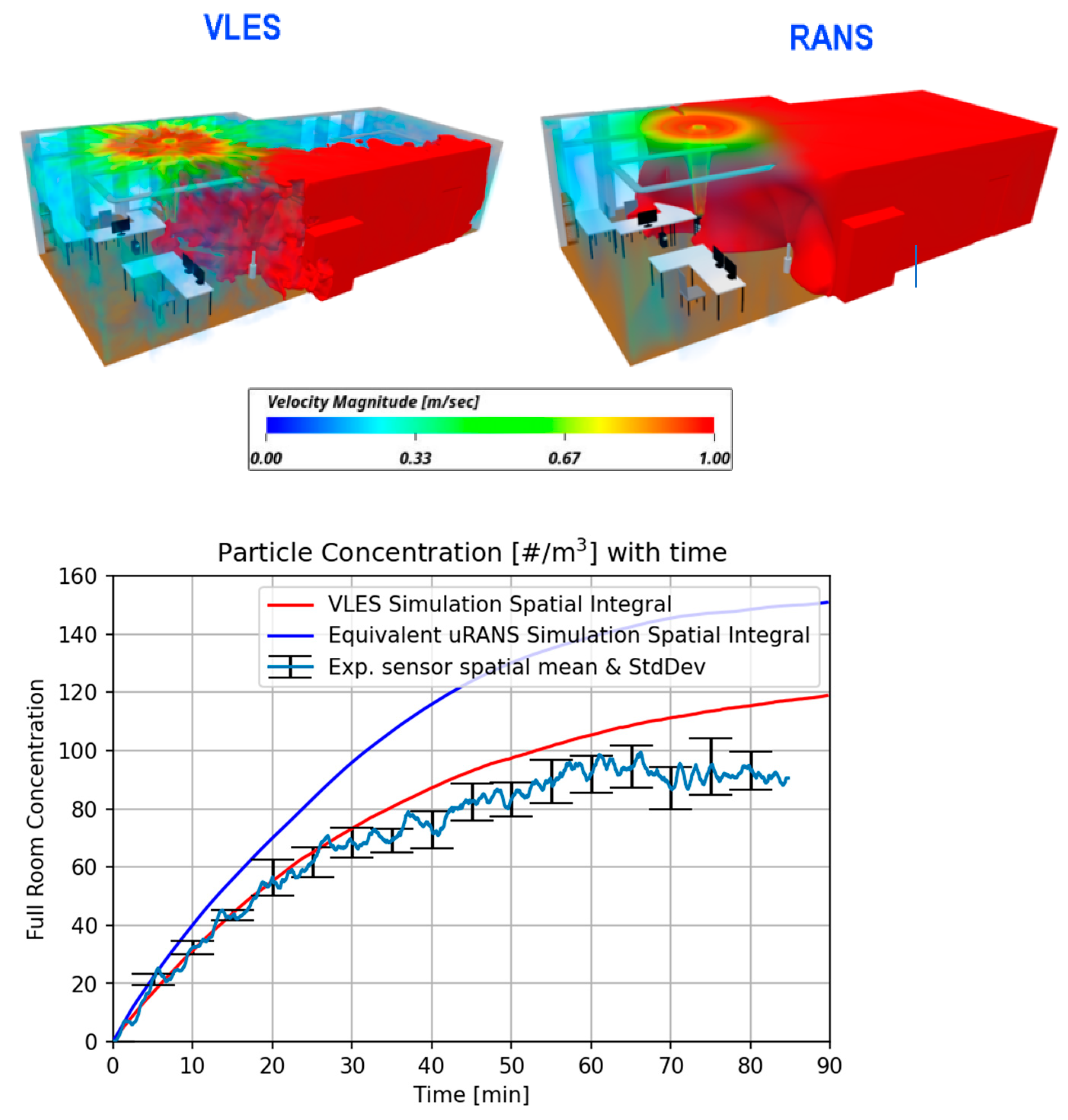
2.2. Simulation Setup

A three-dimensional representation of the room was prepared based on a detailed room measurement and made ready for simulation with 3DEXPERIENCE™ computer aided design (CAD) tools, before being meshed with the PowerDELTA™ tool. The geometry used for the simulation is shown in Figure 2.
In order to account for conduction and room thermal inertia, the doors, ceiling, floor and walls are modelled as multi-layer material, with an appropriate thickness for each layer. A concrete material with a surface absorptivity of 0.7 is used for all the walls of the office, with thickness ranging from 10 to 85 mm depending on the location of the wall. The windows are modelled as transparent materials, and combined with the relevant weather conditions and exterior shading to obtain the correct thermal and solar radiation, wind speed and humidity. Single-glazed glass panels of 6 mm thickness are used to represent the windows. The side of the building with the windows is exposed to the ambient air. The effect of the wind speed, wind direction and relative humidity are read from a weather file and updated during the simulation. Based on the building latitude and longitude, the sun position and solar load are calculated and altered during the course of the simulation. The thermal radiation from the heat sources inside the office room and the direct and diffuse solar radiation from the sun are modelled in detail in this study.
Appropriate heat inputs are applied for all the computers, lighting fixtures and monitors in the room as a function of the time of day. Considering standard hardware under an engineering working load in an office environment, during the day the computer radiates 40 W, the screens 30 W and the lights 35 W. The room is heated with the five radiators placed in the corners. During the night, all devices are turned off. As a result, the correct buoyancy effects are included in the simulation. The locations of the experimental measurement devices are matched in the simulation with simulation probes.
The air cleaners are modelled as mass flow inlets and outlets, with the inlets on the sides of the devices, and the outlet at the top, as shown in Figure 3. The outlet has been modelled as a uniform surface with an area of 0.047 m2 and an average velocity of 2.97 m/s, while the inlets have a total surface area of 0.257 m2 and an average velocity of 0.5 m/s. A separate study was carried out to ensure that the modelled outlet boundary condition correctly reproduced the experimentally measured velocity profile across the outlet section. The flow pattern shows the expected behavior, with an upwards but tilted flow distribution, with enhanced local mixing due to turbulent effects, that quickly dissipates before reaching the ceiling and expanding into the rest of the room. The air released from the top of the air cleaners hits the ceiling, spreads along the side walls, and mixes in the room. Higher amplitudes of velocity and vorticity are typically observed in the upper portions of the room and in the region near the air cleaners.
The inherently transient Lattice Boltzmann-based PowerFLOW™ solver is coupled with the finite difference PowerTHERM™ solver to model all the three modes of heat exchange inside the room [19,20]. The pressure and velocity fields are solved using the Lattice Boltzmann equation, described extensively in existing LBM literature [21,22,23,24,25,26]. The LBM fundamental equation is the Boltzmann equation defined as:
f δ t + u · f = Ω
where f x , t is the particle distribution function (rather than a specific particle). Ω is the collision operator, which relaxes the distribution towards its equilibrium state and includes the interaction of the fluid with solids or turbulence effects. The expression can be re-expressed as the Lattice Boltzmann equation by discretizing in velocity space ξ , to give the form as a function of a finite number of particle velocities. This limits the motion of the particle distributions to a predefined set of directions and speeds. The Boltzmann equation is thus expressed as a set of algebraic equations describing the probability distribution at each state, fi:
f i t + Δ t , x + ξ i Δ t =   f i t , x + Ω i t , x
The temperature equation is solved using an LBM scheme and is fully coupled with the mass conservation and momentum equations, also including effects from buoyancy. For a high Reynolds number, VLES turbulence modelling [27] is incorporated into the Lattice Boltzmann-based solver with a turbulent relaxation time that models the effect of chaotic motion on the statistics of fluid particles collisions.
The PowerFLOW solver also benefits from an integrated Lagrangian particle simulator which includes splash [28], breakup [29] and re-entrainment [30] models. The splash model used determines impinging splash or deposit based on the energy of the impact. The angle of incidence together with this energy is also used to determine the size of the resultant splashed particles. These particles are not to be confused with those discussed above, which are used to describe the carrying medium (air in this case). These particles are not limited to discrete velocities and are dilute; we do not therefore need to consider collisions between these Lagrangian particles. The trajectory of particle motion through air is predicted based on the local drag force acting on the particles, the pressure gradient force, as well as the mass and gravity. The trajectory of the Lagrangian particles is predicted by the following equation:
m D u P a r t i c l e D t = 1 2 ρ C D A u P a r t i c l e u · u P a r t i c l e u + m g
where m is the particle mass, u P a r t i c l e the particle velocity, C D is the particle drag, g is the gravity, ρ the density of the particle and A the particle cross-sectional area. The particles are assumed to be spherical and the drag coefficient is based on the Reynolds number and the Schiller–Naumann correlation [31].
R e = ρ d p u P a r t i c l e u μ g
The full coupling between the Lagrangian particle simulator and PowerFLOW allows us to track the trajectory of millions of particles accurately. During the thermal coupling process, the PowerFLOW exchanges fluid temperature and heat transfer coefficient with PowerTHERM, which in turn returns the surface temperature results to PowerFLOW. Figure 4, shows the PowerFLOW–PowerTHERM coupling process. While a second level of coupling to a system modelling solver, such as Dymola ™, has also been implemented for past building simulations [32] to capture the effects of the HVAC system, this is not required here as the HVAC and rest of the building remain sealed off.

3. Results and Discussion

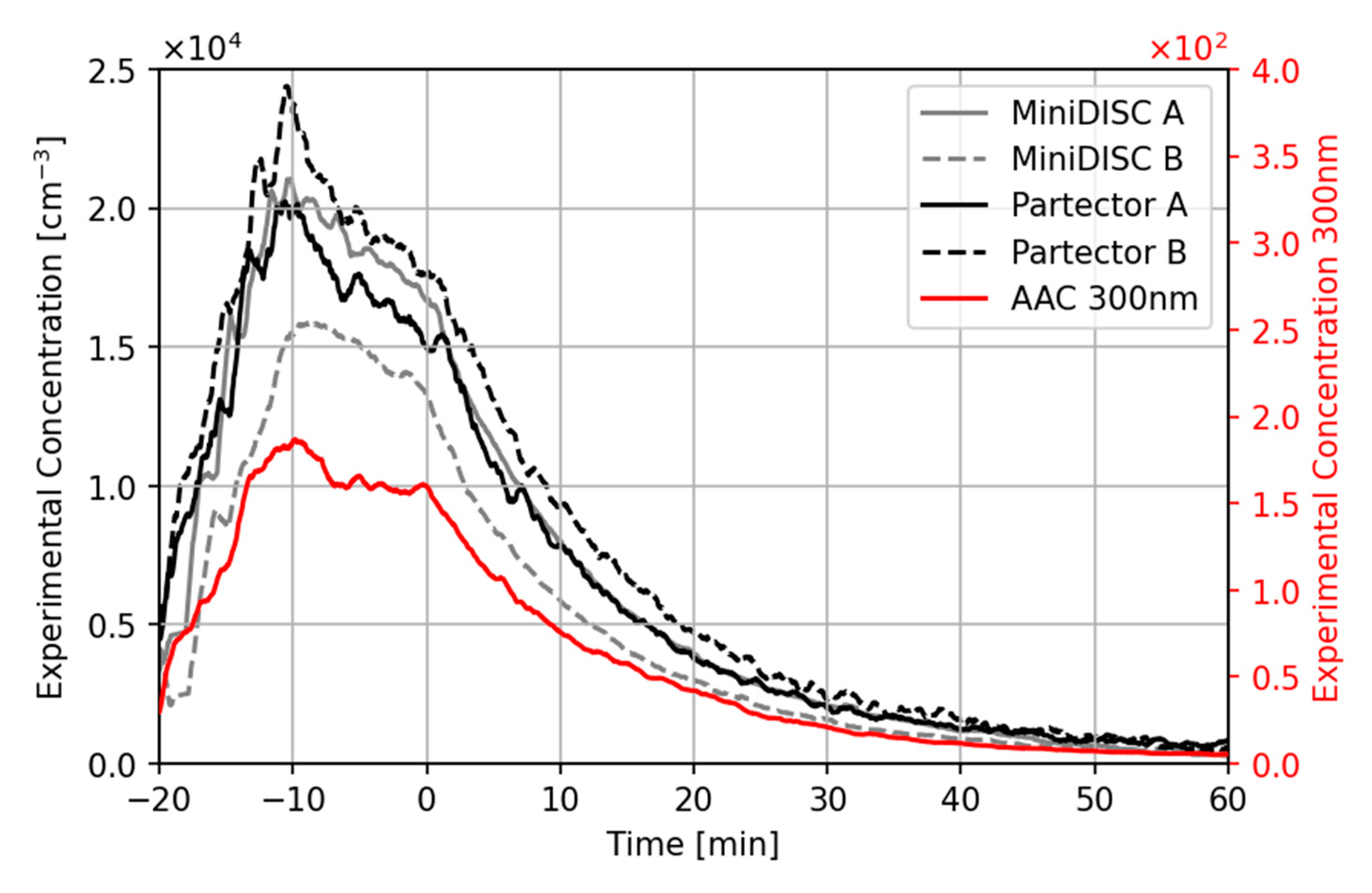
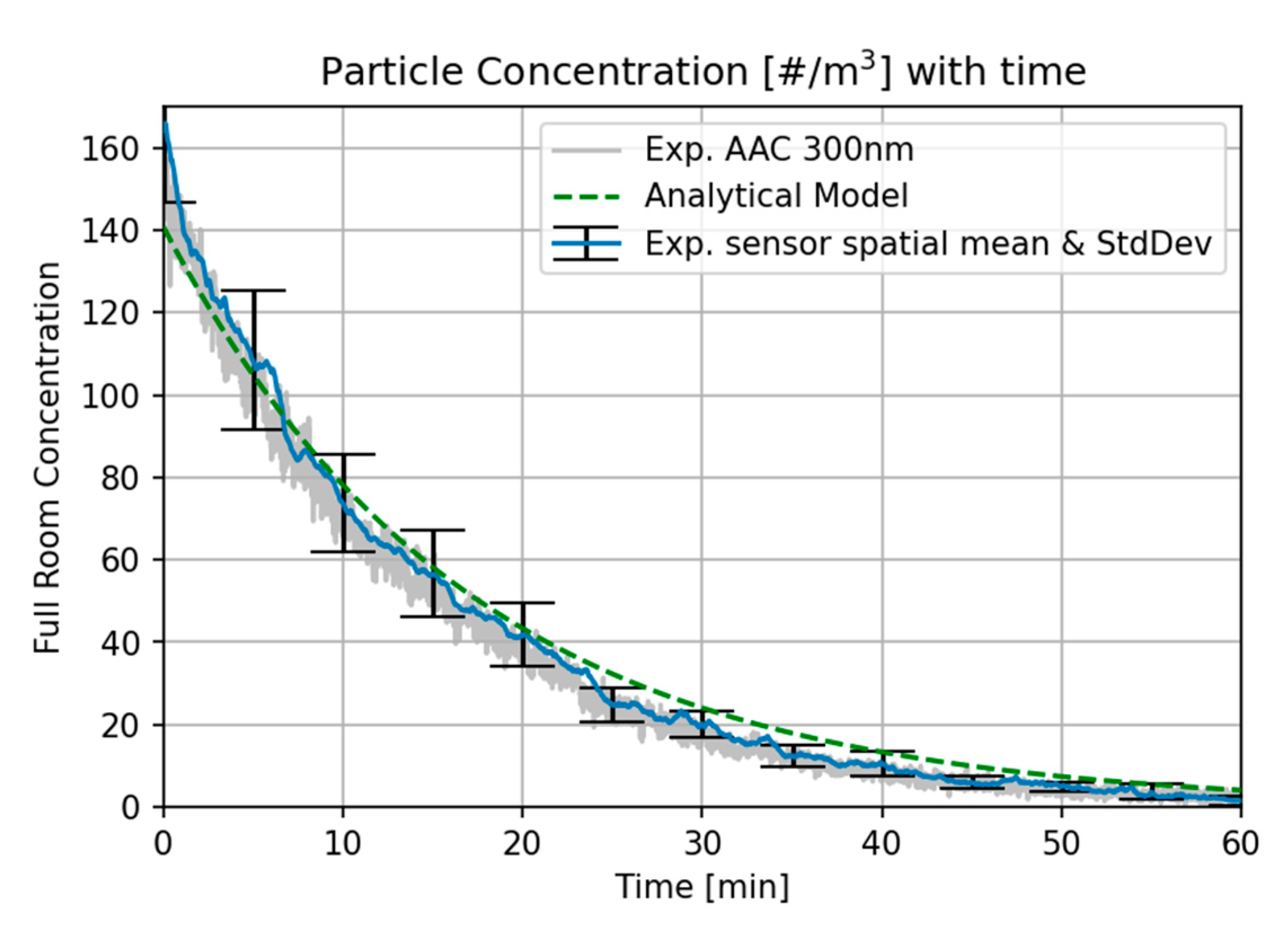
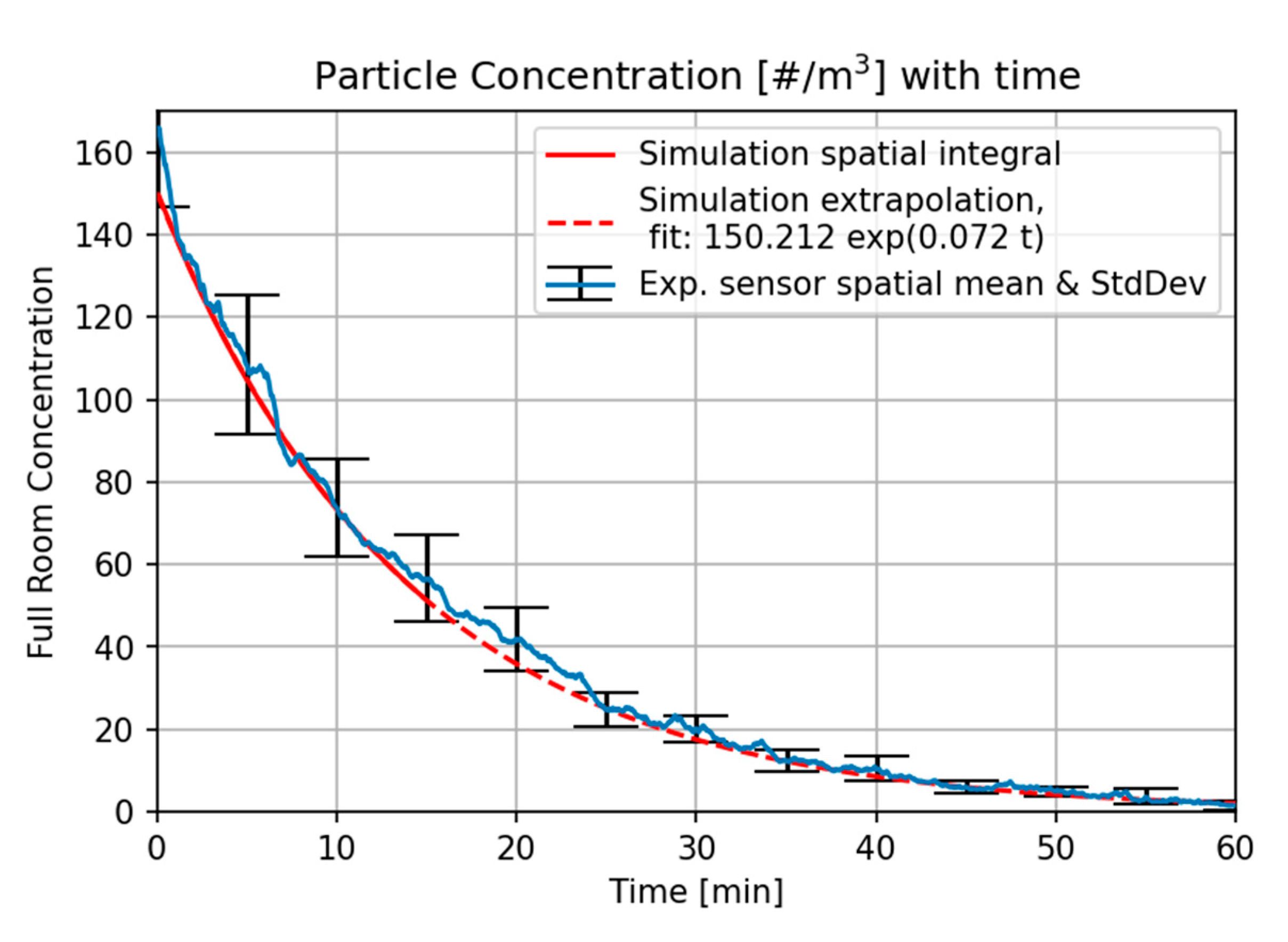
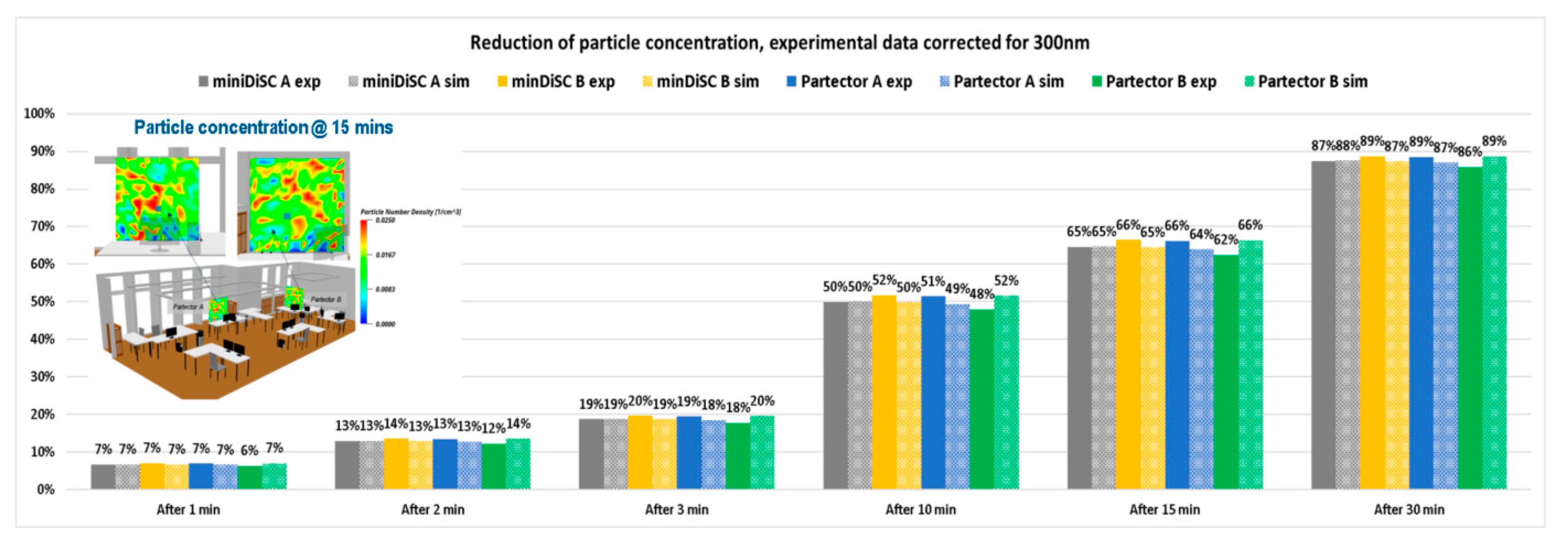
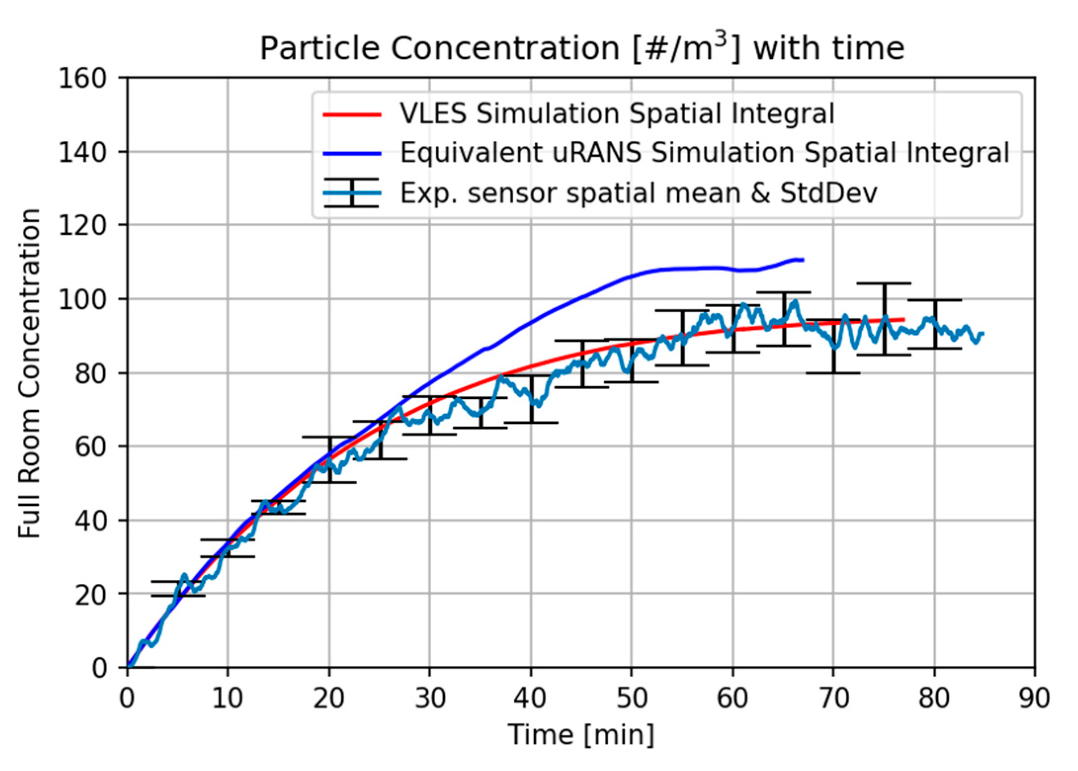
3.1. Validation of Simulated Particle Modelling

3.1.1. Room Clearing Scenario

At the start of the test, the atomizer was operated to emit polydisperse particles with a modal diameter around 100 nm into the room. The emission rate of 300 nm-sized particles was determined to be 1.31 × 10⁷ s−1 at an atomizer pressure of 1 bar and 9.27 × 10⁷ s−1 at a pressure of 3 bar, by measuring the steady-state particle concentration for the operation of an air cleaner with a known CADR in a standardized 30 m³ test chamber. The ceiling fan was turned on during the particle generation phase to allow the particles to homogeneously disperse in the room. The measurement equipment readings confirmed a homogenous distribution of particles with a close-to-constant particle concentration across all measurement devices, as shown in Figure 5, which is in line with previous experimental findings [33,34,35]. At this point, the ceiling fan was turned off and the two air cleaners were turned on so that there was no additional forced convection in the room beyond the effect from the air cleaners themselves. The time at which the air cleaners were turned on marks the t = 0 time, and defines the initial condition of the simulation.
The 300 nm-sized particles investigated here are expected to be convected with room currents, with a small number of particles also being deposited on surfaces due to gravity and diffusion. The addition of the air cleaners causes an additional CADR in the room. Assuming that no recirculation occurs in the room, and that the effects of gravity are negligible, we can estimate an analytical room-clearing curve:
C t = C 0 · e C A D R V · t
where C t is the particle concentration in the room, C 0 the initial room concentration, and   V the room volume [36,37]. Figure 6 shows the room averaged concentration. The results from the AAC device are marked in grey, while the results from all other measurement devices are averaged out in space and time with a moving average to produce the blue curve. The error bars are computed from the spatial differences observed across the room, and represent the standard deviation across the room.
The simulation objective is to confirm that the simulation is able to capture the correct decay rates of particles averaged across the room as well as spatial variations in the decay rate measured across the four room locations. To ensure a high accuracy of results with VLES modelling, a convergence study was conducted to ensure that the relevant physical length scales were accurately captured by the employed grid.
Figure 7 shows the example and result displaying the tracking of some of the simulated particles.
Figure 8 shows the comparison of the averaged 300 nm particle decay curve over time between test, simulations and analytical expectations. All results were normalized to the same initial concentration. The simulation was carried out for 30 min, and the results extrapolated for the remaining experimental time. Very good agreement was obtained between all three cases for the 300 nm concentration of the particles in the room. The slope of the decay curve matches very well both the test and the simulation.
The spatial distribution of the particles is also recorded and compared with the test at the four experimental locations. The spatial distribution is important to understand the risk of exposure from the particles in different places over a certain time. The variation of particles with space, compared to simulation results, is shown in Figure 9. The air cleaners remove about 85 % of the particles after 30 min. This further reduces to 98 % after 60 min and this decrease in particle concentration is seen on all the measuring devices in both the experiment and the simulation. A small difference in percentage of particle reduction between the test and simulation is mainly seen up to 30 min. This remains within the expected accuracy of the experimental measurements, and can also be explained by large spatial variations made visible in the simulation plane plots seen in Figure 9.
The initial activation of the air filtration devices, as well as the associated highly turbulent flow in their vicinity, generates particle motion leading to an inhomogeneous particles distribution early on in the experiment. As time progresses, a homogenous distribution is developed in the room. Nevertheless, the initial variation in particle concentration can affect the cumulative personal exposure of individuals within the room. Table 1 and Figure 10 show the cumulative particle exposure over time at different measurement locations corresponding to co-worker sitting locations, integrated over a volume around their expected head location. The highest exposure is seen at location 1, whereas the lowest exposure is observed at location 4, owing to the specific air cleaner positions and the room geometry. With a standard deviation across cumulative personal exposures for all probes at 30 min of 702 m−3s, and a spatial average of 13,056 m−3s, location 1 levels are beyond one standard deviation above the overall average. From these results, it can be concluded that filter location and room geometry can be optimized to reduce cumulative personal exposure.

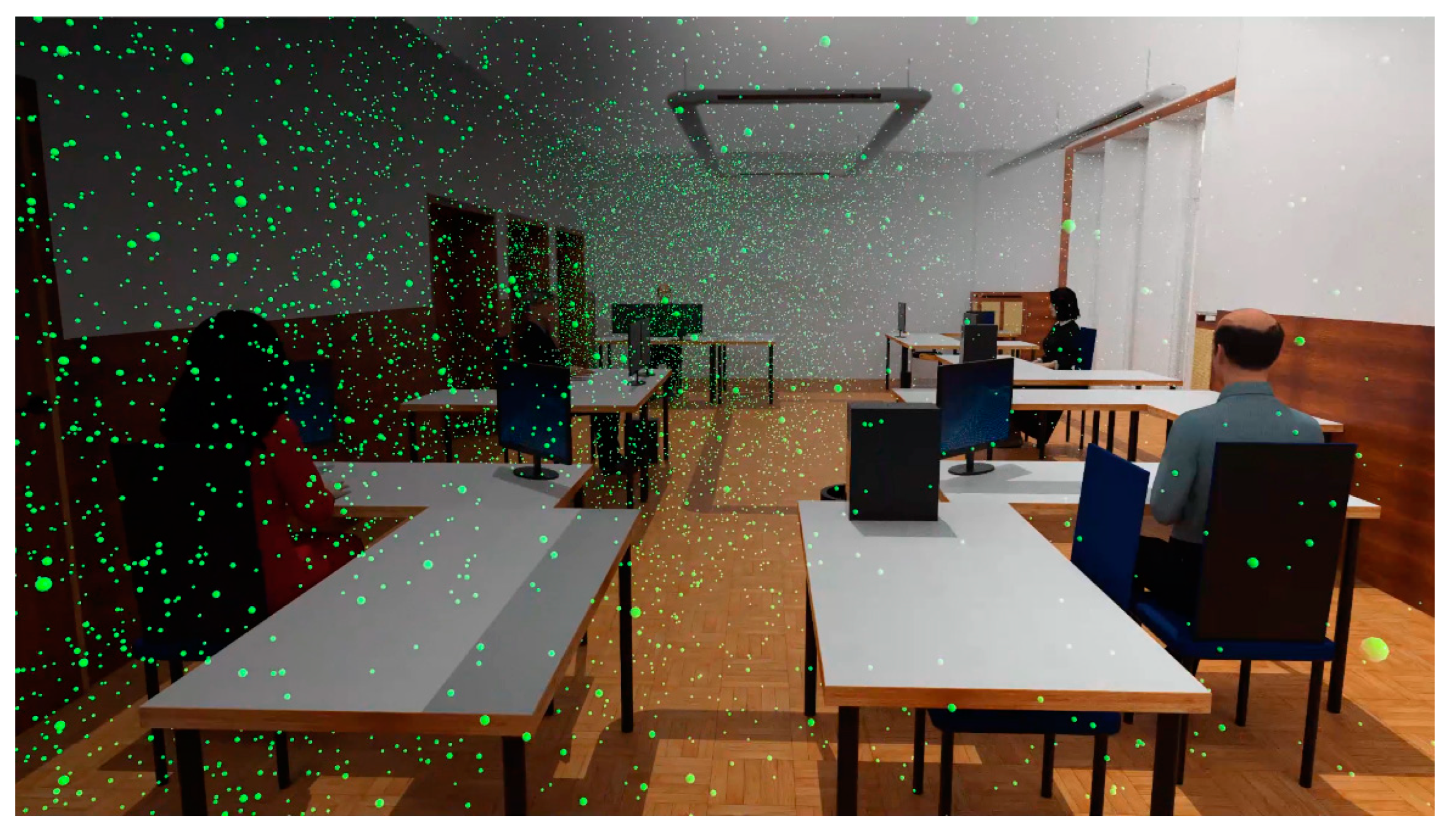
3.1.2. Room Seeding Scenario

In the second validation scenario, particles were seeded into an empty room and the rate of particle increase inside the room over time was compared between the experiment and the simulation. This corresponds, for example, to a scenario with an infectious person continuously emitting virus-laden particles into a room. The experimental setup remained the same as in the room clearing case, with the exception that one air cleaner with a CADR of 550 m3/h was already turned on during the particle generation phase. The simulation was carried out with both scalar transport and particle-modelling approaches, with the scalar transport model neglecting the two-way flow and particle coupling, as well as the effects of gravity on particle deposition. The simulation was also conducted with the VLES activated, but with large-scale structures modelled in a similar fashion to subgrid-scale structures, as opposed to being accurately resolved. While accurately resolved large-scale structures provide the expected VLES results shown previously, using modelling for large scales provides results akin to an unsteady Reynolds averaged Navier–Stokes (uRANS) method [25,38,39]; for simplicity, this will be referred to as equivalent uRANS in the following sections. An example velocity distribution comparing the VLES and equivalent uRANS is shown in Figure 11. The flow exiting from the top of the air filter hits the ceiling and spreads across the room. The flow is more concentrated in the equivalent uRANS simulation compared to the VLES. In the VLES, the turbulence effects on the flow are more pronounced, and there is a good flow spread and mixing inside the room. Less mixing and distribution of flow is observed in the equivalent uRANS simulation, especially close to the floor.
The spatially averaged particle accumulation over time for all the four simulations is compared with experimental results in Figure 12 and Figure 13. Starting with the scalar modelling results of Figure 12, neither the VLES nor the equivalent uRANS results are able to capture the expected concentration stabilization caused by the natural decay of particles in the room. In addition to this, the equivalent uRANS results also provide less accurate results when matching the experimental curve slope. When we look at spatial distribution, the equivalent uRANS results also show a more homogenous distribution of particles in the top right corner of the room, owing to inaccurately represented turbulent flow from the air filtration device.
Figure 13 shows the particle modelling distribution, comparing experimental results with the VLES and equivalent uRANS models. The slope of the particle accumulation curve for the VLES model agrees closely with the test, while the equivalent uRANS mode overshoots the predictions. Furthermore, compared to the scalar transport model, the slope of the VLES particle concentration curve agrees very well with the test, indicating that VLES simulation with particle modelling is capable of capturing the accurate behavior of the seeding and filtering of particles in a room under forced convection effects.

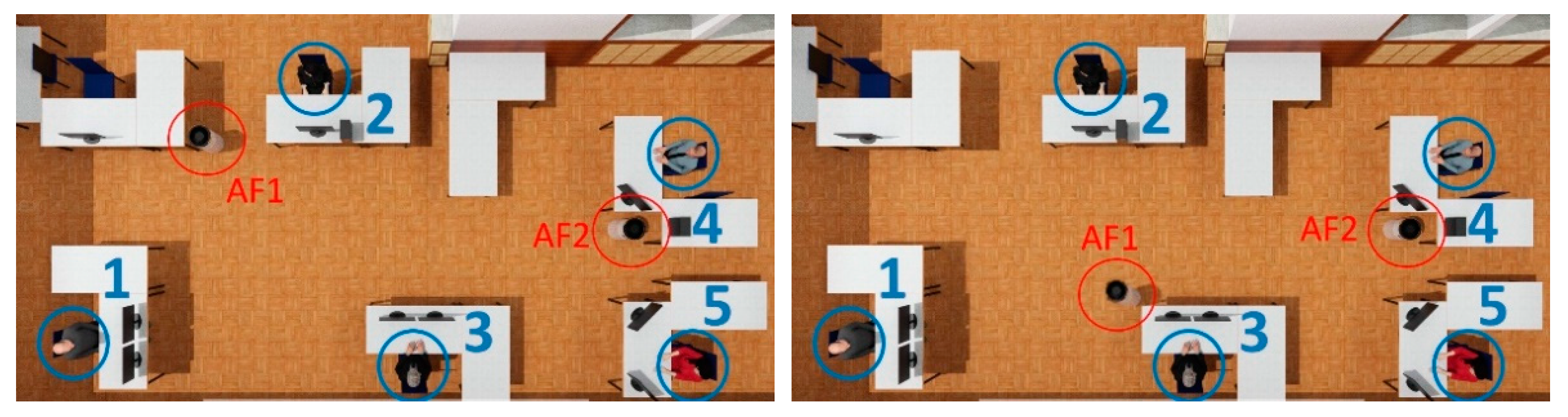
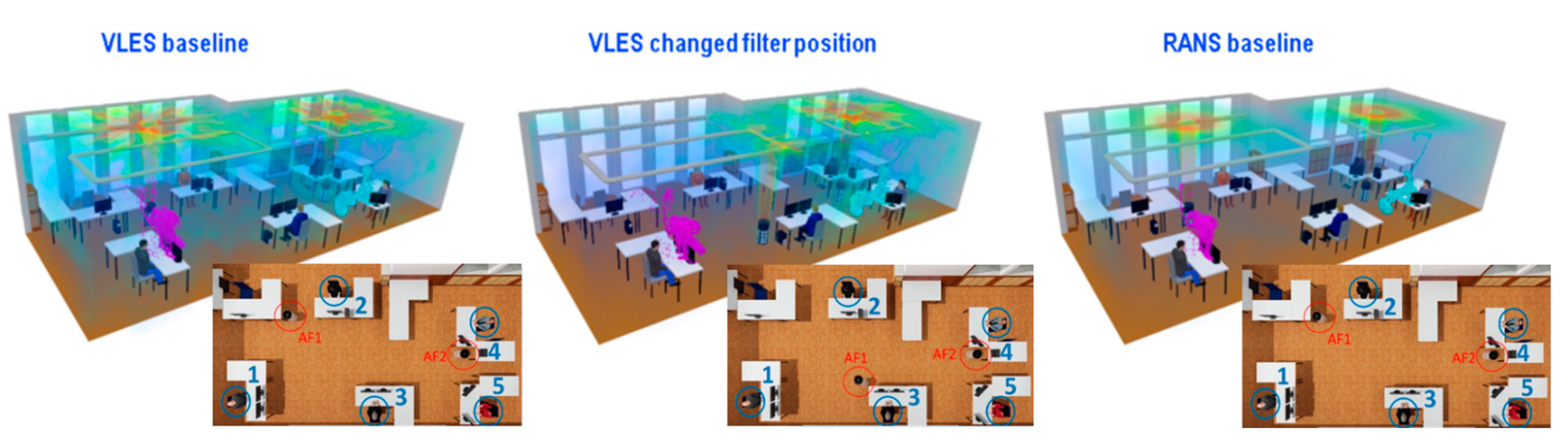
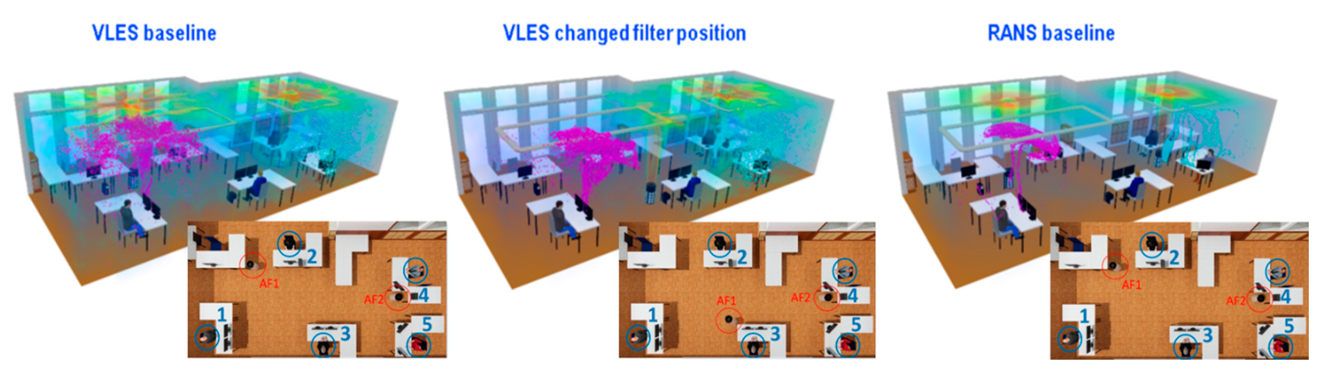
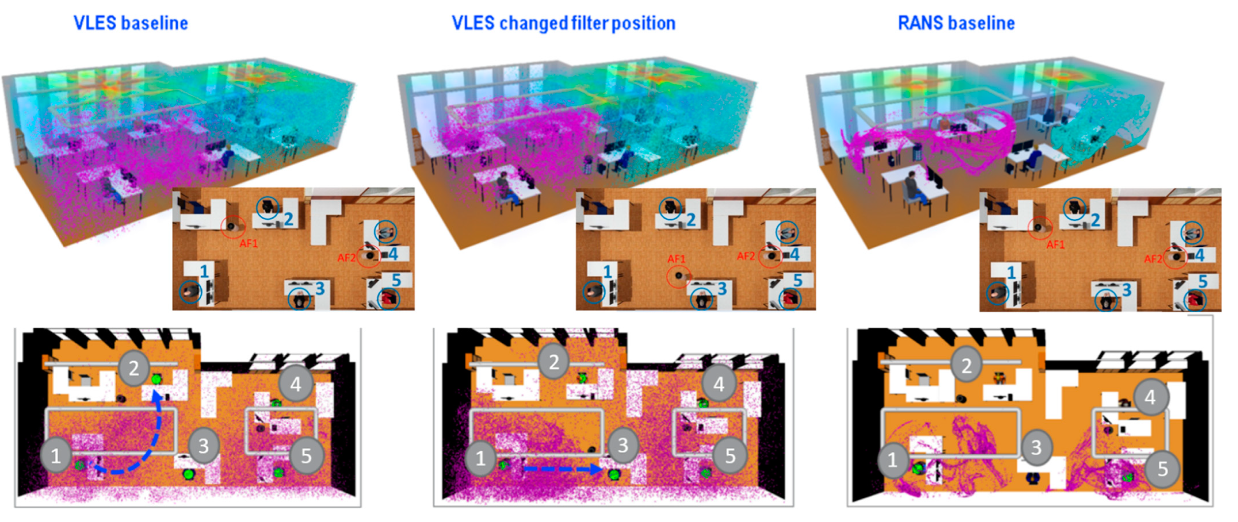
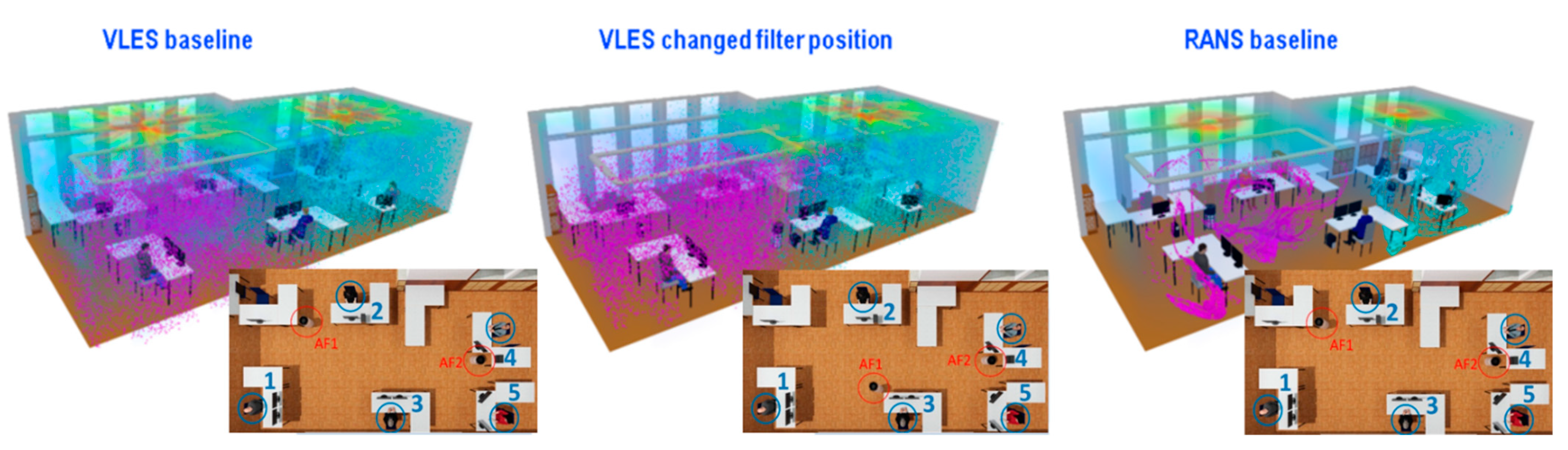
3.2. Leveraging Simulation to Improve Room Layouts: Coughing Scenario

A cough simulation was carried out with occupants inside the room for two different positions of the air cleaners; this simulation could not be compared to experimental results, as coughing could not be mimicked experimentally. In the simulation, five occupants were introduced into the room and particles were emitted by two coughing occupants seated across the room; the particles were monitored over time to assess the risk of exposure for all the other occupants. Figure 14 shows all the room occupants, as well as two possible variations for the position of the air filter 1 (AF1). In this simulation, both air cleaners were turned on and the flow rate was set to 500 m3/h. The simulation was carried out for 2 min to predict the cumulative personal exposure of each occupant shortly after the coughing event. In the baseline filter position, the coughing simulation was carried out with both the VLES and equivalent uRANS approaches, while only the VLES was used for the changed position of the air cleaners.
The information required to set up the cough simulations shown in this paper was collected from several sources. The cough is a double cough while the flow rate variation over time is taken from Figure 8 in [40]. The mouth opening size was approximately 5 cm2, which is the average mouth opening size recorded for a male in [40].
The particle size distribution was fitted to the diameter data from Figure 2 of [41]. The information for the release rate of the particles was also taken from [41], with 1.37 x10⁷ particles being released per cough. Most of these particles were of a smaller size than those measured by other studies [42]. In the present paper, the cough was set up with a mean particle size of 320 nm, with particles sizes varying between 270 nm and 370 nm.
Male 1 and female 5 cough and emit particles inside the room for a period of 0.6 s, starting 2.5 s after the beginning of the simulation. The particles emitted by the two occupants travel along different paths and spread inside the room. In this simulation, both the coughing occupants are facing forward, and the angle of emission is 0°. This results in the emitted particles falling in front of the emitters. Some of the heavier particles settle on computer surfaces, tables and the ground. The lighter particles are carried away by the flow. Figure 15 shows the particle distribution after 25 s for all three scenarios. The particles released from coughing male 1 hit the monitors in front of him and rise up. More fomite deposition is seen on the monitors in front of coughing male 1, while the path of particles emitted from coughing female 5 is not altered by any objects, allowing particles to propagate more freely. The particle distribution is similar after 25 s for all three cases.
After 50 s, in the baseline VLES model, the particles from male 1 rise up towards the ceiling and start spreading inside the room as shown in Figure 16. The particles released from female 5 are pulled towards the air filter. A part of these is sucked in and the rest is entrained by the outlet flow to spread across the room. These particles then travel and spread in the region of the coughing female 5. A similar behavior is observed for the particles released from female 5 in the VLES model with a changed filter position. However, the particles emitted from coughing male 1 do not directly travel to air filter AF1. The particles are carried upwards by the flow after interacting with the monitors. In the equivalent uRANS model, the behavior of the particle movement is the same as in the VLES model, but the particles emitted from the two occupants (male 1 and female 5) remain more clustered. Due to the localized high flow velocities near the filters, these particles do not travel far. In all the results, the particles released from both emitters have not yet reached the other occupants and there is no risk of contamination.
The particles continue to travel farther into the room in the VLES simulations. After 75 s, shown in Figure 17, the particles are now in close proximity of other occupants. In the baseline VLES results, the particles from coughing male 1 rise upwards and travel towards the other side of the room, where the air filter AF1 is placed, close to female 2. Similarly, for the VLES model with a changed filter position, the particles from the coughing male 1 rise up, spread in the upper area, and then travel towards air filter AF1 placed next to male 3. Due to this, the cumulative personal exposure for occupants 2 and 3 will vary as a function of the location of AF1: Female 2 is likely to receive more particles from male 1 in the baseline VLES simulation, whereas male 3 will receive more particles from male 1 in the VLES simulation with a changed filter position. The risk of exposure from particles released by female 5 is similar in both VLES models.
In the equivalent uRANS model, the particles from female 5 are not spread across the room and remain more concentrated around the emitter’s vicinity. The particles from male 2 spread towards male 3. None of the particles reach the other occupants in the equivalent uRANS model, whereas some particles are now in close proximity to other occupants in both VLES models.
Figure 18 shows the particle distribution after 120 s. The particles are well mixed in the baseline VLES and the changed filter position VLES simulations. In the baseline VLES results, male 4, sitting in the corner next to coughing female 5, receives the highest particle concentration. He is followed by female 2 sitting next to the air filter AF1, and male 3 sitting in the center. It can be observed here that the occupants sitting closer to the air cleaners (namely male 4 and female 2) are exposed to more particles than the occupant sitting in the center, between emitters (male 3). Although the air cleaners remove particles from the room with time, they also generate suction, pulling in particles into their close vicinity, which leads to the higher cumulative personal exposures observed for bystanders. This behavior is also observed for the VLES model with the changed filter position wherein male 3 sitting in the center and close to air filter AF1 is exposed to more particles. He is closely followed by male 4 sitting next to the second air filter AF2 on the other side, close to coughing female 5.
After 120 s, the equivalent uRANS model still shows particles remaining clustered around the emitter region, indicating a low risk of exposure for the other occupants. Unlike the VLES model, the equivalent uRANS model does not accurately represent a realistic forced convection scenario, and there is little or no occupant’s exposure to the coughed particles.
Figure 19 shows the cumulative personal exposure of the occupants from the particles emitted from coughing. Comparing baseline and changed filter location VLES simulations, it can be seen that altering the filter position increases the cumulative personal exposure of the room occupants. As discussed previously, occupants sitting closer to the air filters are exposed to higher quantities of particles in both baseline and changed filter position VLES models.
From these results, it can be concluded that the new AF1 air filter position, placed between male 3 and male 1, is detrimental. In this scenario, the effective particle filtering rate is reduced due to recirculation, and the cumulative personal exposure of the occupants is increased. Therefore, it is recommended that the air filter be placed further away from occupants when possible.

4. Conclusions

In this paper, we compared experimental results for the distribution of particles in the size range of exhaled, potentially virus-laden, droplets to simulation results from a Lattice Boltzmann solver for both a room clearing and room seeding case. In both cases, the simulations were able to accurately capture the particle concentration change in the room. Furthermore, spatial variations in the particle concentration also compared favorably between the simulation and the experiment. It was shown that approaches modelling large-scale turbulence rather than accurately resolving grid-scale structures showed a large deviation from the average room particle count and growth rate. As showcased in past literature, we would not recommend uRANS or RANS approaches for modelling particle propagation under forced convection effects, when no randomizing velocities have been added.
The second part of the paper dealt with the usage of simulation to improve the positioning of filtering devices. While filtering devices always reduce the cumulative personal exposure of individuals within the room, it was shown that the location of air filtration devices can also have an impact. Individuals positioned close to the air cleaners showed increased levels of cumulative personal exposure in both coughing scenarios. The impact of this was observed in the first few minutes after the coughing event, before the forced convection had spread particles across the room.
This validation and demonstration of the benefits of simulation is an initial point of research, which is expected to evolve towards systematic optimization of air quality in built environments. While these examples only portrayed the effects of standalone air cleaners, it is expected that the same approach can be applied to HVAC system installations, optimizing the location of inlets and outlets for maximum safety. This can then be combined with human comfort and energy efficiency estimations in order to help balance all three attributes simultaneously.

Author Contributions

Conceptualization, C.M.A.L. and C.A.; methodology, C.M.A.L., J.J., S.S., A.M.T. and C.A.; validation, F.Q. and C.M.A.L.; formal analysis, F.Q. and C.M.A.L.; investigation, S.S., C.A., A.M.T., F.Q., V.N. and C.M.A.L.; resources, C.M.A.L.; data curation, J.L., F.Q. and C.M.A.L.; writing—original draft preparation, V.N. and C.M.A.L.; writing—review and editing, C.M.A.L., C.A., S.S., F.Q. and J.J.; visualization, F.Q.. All authors have read and agreed to the published version of the manuscript.

Funding

This research received no external funding.

Institutional Review Board Statement

Not applicable.

Informed Consent Statement

Not applicable.

Data Availability Statement

Not applicable.

Conflicts of Interest

The authors declare no conflict of interest.

References

  1. Morawska, L.; Cao, J. Airborne Transmission of SARS-CoV-2: The World Should Face the Reality. Environ. Int. 2020, 139, 105730. [Google Scholar] [CrossRef]
  2. Zhang, R.; Li, Y.; Zhang, A.L.; Wang, Y.; Molina, M.J. Identifying Airborne Transmission as the Dominant Route for the Spread of COVID-19. Proc. Natl. Acad. Sci. USA 2020, 117, 14857–14863. [Google Scholar] [CrossRef]
  3. Somsen, G.A.; van Rijn, C.; Kooij, S.; Bem, R.A.; Bonn, D. Small Droplet Aerosols in Poorly Ventilated Spaces and SARS-CoV-2 Transmission. Lancet Respir. Med. 2020, 8, 658–659. [Google Scholar] [CrossRef]
  4. Asbach, C.; Held, A.; Kiendler-Scharr, A.; Scheuch, G.; Schmid, H.-J.; Schmitt, S.; Schumacher, S.; Wehner, B.; Weingartner, E.; Weinzierl, B.; et al. Position Paper of the Gesellschaft Für Aerosolforschung on Understanding the Role of Aerosol Particles in SARS-CoV-2 Infection; Association for Aerosol Research: Raleigh, NC, USA, 2021. [Google Scholar] [CrossRef]
  5. Held, A.; Dellweg, D.; Köhler, D.; Pfaender, S.; Scheuch, G.; Schumacher, S.; Steinmann, E.; Weingartner, E.; Weinzierl, B.; Asbach, C. Interdisciplinary Perspectives on the Role of Aerosol Transmission in SARS-CoV-2 Infections. Gesundh. Bundesverb. Arzte Offentlichen Gesundh. Ger. 2022, 84, 566–574. [Google Scholar] [CrossRef]
  6. Scheuch, G. Breathing Is Enough: For the Spread of Influenza Virus and SARS-CoV-2 by Breathing Only. J. Aerosol Med. Pulm. Drug Deliv. 2020, 33, 230–234. [Google Scholar] [CrossRef]
  7. Mittal, R.; Ni, R.; Seo, J.-H. The Flow Physics of COVID-19. J. Fluid Mech. 2020, 894, F2. [Google Scholar] [CrossRef]
  8. Bourouiba, L.; Dehandschoewercker, E.; Bush, J.W.M. Violent Expiratory Events: On Coughing and Sneezing. J. Fluid Mech. 2014, 745, 537–563. [Google Scholar] [CrossRef]
  9. Succi, S. The Lattice Boltzmann Equation: For Fluid Dynamics and Beyond; Clarendon Press: Oxford, UK, 2001; ISBN 978-0-19-850398-9. [Google Scholar]
  10. Duda, B.M.; Laskowksi, G.M. Lattice-Boltzmann Very Large Eddy Simulations of the NASA Juncture Flow Model. In AIAA Scitech 2020 Forum; AIAA SciTech Forum; American Institute of Aeronautics and Astronautics: Reston, VI, USA, 2020. [Google Scholar]
  11. Ahmadzadeh, M.; Shams, M. Multi-Objective Performance Assessment of HVAC Systems and Physical Barriers on COVID-19 Infection Transmission in a High-Speed Train. J. Build. Eng. 2022, 53, 104544. [Google Scholar] [CrossRef]
  12. Wang, M.; Lin, C.-H.; Chen, Q. Advanced Turbulence Models for Predicting Particle Transport in Enclosed Environment. Build. Environ. 2012, 47, 40–49. [Google Scholar] [CrossRef]
  13. Ivanova, E.; Noll, B.; Aigner, M. RANS and LES of Turbulent Mixing in Confined Swirling and Non-Swirling Jets. In Proceedings of the 6th AIAA Theoretical Fluid Mechanics Conference, Honolulu, HI, USA, 27–30 June 2011. [Google Scholar]
  14. Chen, Q. Ventilation Performance Prediction for Buildings: A Method Overview and Recent Applications. Build. Environ. 2009, 44, 848–858. [Google Scholar] [CrossRef]
  15. Blocken, B. LES over RANS in Building Simulation for Outdoor and Indoor Applications: A Foregone Conclusion? Build. Simul. 2018, 11, 821–870. [Google Scholar] [CrossRef] [Green Version]
  16. Fierz, M.; Meier, D.; Steigmeier, P.; Burtscher, H. Aerosol Measurement by Induced Currents. Aerosol Sci. Technol. 2014, 48, 350–357. [Google Scholar] [CrossRef] [Green Version]
  17. Todea, A.M.; Beckmann, S.; Kaminski, H.; Asbach, C. Accuracy of Electrical Aerosol Sensors Measuring Lung Deposited Surface Area Concentrations. J. Aerosol Sci. 2015, 89, 96–109. [Google Scholar] [CrossRef]
  18. Burr, K.P.; Akylas, T.R.; Mei, C.C. Chapter Two Two-Dimensional Laminar Boundary Layers; Springer: Berlin/Heidelberg, Germany, 2014. [Google Scholar]
  19. Chen, S.; Doolen, G.D. Lattice Boltzmann Method for Fluid Flow. Annu. Rev. Fluid Mech. 1998, 30, 329–364. [Google Scholar] [CrossRef] [Green Version]
  20. Ferziger, J.H.; Kaper, H.G. Mathematical Theory of Transport Processes in Gases. Am. J. Phys. 1973, 41, 601–603. [Google Scholar] [CrossRef]
  21. Zhou, Y.; Zhang, R.; Staroselsky, I.; Chen, H. Numerical Simulation of Laminar and Turbulent Buoyancy-Driven Flows Using a Lattice Boltzmann Based Algorithm. Int. J. Heat Mass Transf. 2004, 47, 4869–4879. [Google Scholar] [CrossRef]
  22. Li, Y.; Shock, R.; Zhang, R.; Chen, H. Numerical Study of Flow Past an Impulsively Started Cylinder by the Lattice-Boltzmann Method. J. Fluid Mech. 2004, 519, 273–300. [Google Scholar] [CrossRef]
  23. Bhatnagar, P.L.; Gross, E.P.; Krook, M. A Model for Collision Processes in Gases. I. Small Amplitude Processes in Charged and Neutral One-Component Systems. Phys. Rev. 1954, 94, 511–525. [Google Scholar] [CrossRef]
  24. Chapman, S. The Mathematical Theory of Non-uniform Gases: An Account Of The Kinetic Theory Of Viscosity, Thermal Conduction and Diffusion. In Gases, 3rd ed.; Cambridge University Press: New York, NY, USA, 1991; ISBN 978-0-521-40844-8. [Google Scholar]
  25. Kotapati, R.; Keating, A.; Kandasamy, S.; Duncan, B.; Shock, R.; Chen, H. The Lattice-Boltzmann-VLES Method for Automotive Fluid Dynamics Simulation, A Review; SAE: Warrendale, PA, USA, 2009. [Google Scholar]
  26. Chen, H.; Chen, S.; Matthaeus, W.H. Recovery of the Navier-Stokes Equations Using a Lattice-Gas Boltzmann Method. Phys. Rev. A 1992, 45, R5339–R5342. [Google Scholar] [CrossRef]
  27. Chen, H.; Kandasamy, S.; Orszag, S.; Shock, R.; Succi, S.; Yakhot, V. Extended Boltzmann Kinetic Equation for Turbulent Flows. Science 2003, 301, 633–636. [Google Scholar]
  28. Mundo, C.H.R.; Sommerfeld, M.; Tropea, C. Droplet-Wall Collisions: Experimental Studies of the Deformation and Breakup Process. Int. J. Multiph. Flow 1995, 21, 151–173. [Google Scholar] [CrossRef]
  29. O’Rourke, P.J.; Amsden, A.A. A Spray/Wall Interaction Submodel for the KIVA-3 Wall Film Model; SAE International: Warrendale, PA, USA, 2000. [Google Scholar]
  30. O’Rourke, P.J.; Amsden, A.A. The Tab Method for Numerical Calculation of Spray Droplet Breakup; SAE International: Warrendale, PA, USA, 1987. [Google Scholar]
  31. Shiller, L.; Naumann, A. A Drag Coefficient Correlation. Z. Ver. Dtsch. Ing. 1935, 77, 318–320. [Google Scholar]
  32. Tumforde, T.; Wischhusen, S.; Nagarajan, V.; Luzzato, C.; Heinrich, A.A.; Lebrun, V.-M.; Mann, A. Balancing Interior Environmental Quality and HVAC Energy Efficiency Using 1D and 3D Simulation; NAFEMS World Congress 2021. In Proceedings of the NAFEMS World Congress 2021, Berlin, Germany, 21 October 2021. [Google Scholar]
  33. Küpper, M.; Asbach, C.; Schneiderwind, U.; Finger, H.; Spiegelhoff, D.; Schumacher, S. Testing of an Indoor Air Cleaner for Particulate Pollutants under Realistic Conditions in an Office Room. Aerosol Air Qual. Res. 2019, 19, 1655–1665. [Google Scholar] [CrossRef] [Green Version]
  34. Szabadi, J.; Meyer, J.; Lehmann, M.; Dittler, A. Simultaneous Temporal, Spatial and Size-Resolved Measurements of Aerosol Particles in Closed Indoor Environments Applying Mobile Filters in Various Use-Cases. J. Aerosol Sci. 2022, 160, 105906. [Google Scholar] [CrossRef]
  35. Curtius, J.; Granzin, M.; Schrod, J. Testing Mobile Air Purifiers in a School Classroom: Reducing the Airborne Transmission Risk for SARS-CoV-2. Aerosol Sci. Technol. 2021, 55, 586–599. [Google Scholar] [CrossRef]
  36. Schumacher, S.; Spiegelhoff, D.; Schneiderwind, U.; Finger, H.; Asbach, C. Performance of New and Artificially Aged Electret Filters in Indoor Air Cleaners. Chem. Eng. Technol. 2018, 41, 27–34. [Google Scholar] [CrossRef]
  37. Schumacher, S.; Banda Sanchez, A.; Caspari, A.; Staack, K.; Asbach, C. Testing Filter-Based Air Cleaners with Surrogate Particles for Viruses and Exhaled Droplets. Atmosphere 2022, 13, 1538. [Google Scholar] [CrossRef]
  38. Chen, H. Large Eddy Simulation of Turbulence Via Lattice Boltzmann Based Approach: Fundamental Physics and Practical Applications. In The Aerodynamics of Heavy Vehicles: Trucks, Buses, and Trains; McCallen, R., Browand, F., Ross, J., Eds.; Springer: Berlin/Heidelberg, Germany, 2004; p. 123. [Google Scholar]
  39. Labois, M.; Lakehal, D. Very-Large Eddy Simulation (V-LES) of the Flow across a Tube Bundle. Nucl. Eng. Des. 2011, 241, 2075–2085. [Google Scholar] [CrossRef]
  40. Gupta, J.K.; Lin, C.-H.; Chen, Q. Flow Dynamics and Characterization of a Cough. Indoor Air 2009, 19, 517–525. [Google Scholar] [CrossRef]
  41. Zayas, G.; Chiang, M.C.; Wong, E.; MacDonald, F.; Lange, C.F.; Senthilselvan, A.; King, M. Cough Aerosol in Healthy Participants: Fundamental Knowledge to Optimize Droplet-Spread Infectious Respiratory Disease Management. BMC Pulm. Med. 2012, 12, 11. [Google Scholar] [CrossRef] [Green Version]
  42. Lindsley, W.G.; Pearce, T.A.; Hudnall, J.B.; Davis, K.A.; Davis, S.M.; Fisher, M.A.; Khakoo, R.; Palmer, J.E.; Clark, K.E.; Celik, I.; et al. Quantity and Size Distribution of Cough-Generated Aerosol Particles Produced by Influenza Patients during and after Illness. J. Occup. Environ. Hyg. 2012, 9, 443–449. [Google Scholar] [CrossRef]
Figure 1. Virtual twin of the office room, with the red circle denoting the location of the atomizer.
Atmosphere 13 02032 g001
Figure 2. Simulated geometry of the office room.
Atmosphere 13 02032 g002
Figure 3. Rendered CFD visualization of the two air cleaning devices in the room. The airflow to the device is shown in yellow and the filtered airflow away from the device in blue.
Atmosphere 13 02032 g003
Figure 4. Scheme of the PowerFLOW–PowerTHERM coupling process.
Atmosphere 13 02032 g004
Figure 5. Concentrations measured with the different instruments before and after switching on the air cleaner at t = 0 min.
Atmosphere 13 02032 g005
Figure 6. Room averaged concentration measured as number of particles per cubic centimeter [#/m3] compared to an analytical model.
Atmosphere 13 02032 g006
Figure 7. Particles at a certain point in time simulated inside room.
Atmosphere 13 02032 g007
Figure 8. Comparison of the analytical, experimental and simulated particle decay curves measured as number of particles per cubic centimeter [#/m3].
Atmosphere 13 02032 g008
Figure 9. Reduction in the particle concentration after different operation times, determined by experiment and simulation.
Atmosphere 13 02032 g009
Figure 10. Overview of the person locations in the room.
Atmosphere 13 02032 g010
Figure 11. Flow distribution differences between VLES (left) and equivalent uRANS (right).
Atmosphere 13 02032 g011
Figure 12. Scalar modelling concentration of particles inside room and comparison between VLES and equivalent uRANS. The red isosurface shows a water vapour mass fraction above 0.0008.
Atmosphere 13 02032 g012
Figure 13. Particle modelling concentration of particles inside room and comparison between VLES and equivalent uRANS.
Atmosphere 13 02032 g013
Figure 14. Geometry of baseline (left) and changed filter position (right). AF1: air filter 1, AF2: air filter 2. The numbering of the people locations in blue remain as previously.
Atmosphere 13 02032 g014
Figure 15. Distribution of the particle concentration for a coughing scenario simulated after 25 s using different simulation methods and positions of the air cleaner.
Atmosphere 13 02032 g015
Figure 16. Distribution of the particle concentration for a coughing scenario simulated after 50 s using different simulation methods and positions of the air cleaner.
Atmosphere 13 02032 g016
Figure 17. Distribution of the particle concentration for a coughing scenario simulated after 75 s using different simulation methods and positions of the air cleaner.
Atmosphere 13 02032 g017
Figure 18. Distribution of the particle concentration for a coughing scenario simulated after 120 s.
Atmosphere 13 02032 g018
Figure 19. Cumulative particle exposure over time. The equivalent uRANS results are not shown as they show no cummulative exposure for non-coughing occupants.
Atmosphere 13 02032 g019
Table 1. Cumulative personal exposure to particles from the simulation results for five different locations in the room.
Cumulative Personal Exposure [m−3s]10 min15 min20 min25 min30 min
Location 1801210,39812,14513,34714,159
Location 27308949311,12612,27513,062
Location 37474977011,30712,43813,100
Location 47576953611,01311,98812,631
Location 57808993411,46712,52113,327
Publisher’s Note: MDPI stays neutral with regard to jurisdictional claims in published maps and institutional affiliations.

