


Comparison of Planetary Boundary Layer Height Derived from Lidar in AD-Net and ECMWFs Reanalysis Data over East Asia
Abstract
:1. Introduction
2. Materials and Methods
2.1. BLH Derived from AD-Net
2.2. BLHs from ECMWFs
3. Results
4. Conclusions
5. Discussion
Author Contributions
Funding
Institutional Review Board Statement
Informed Consent Statement
Data Availability Statement
Acknowledgments
Conflicts of Interest
References
- Arya, S.P. Introduction to Micrometeorology, 2nd ed.; Academic Press: Cambridge, MA, USA, 2001; pp. 1–450. [Google Scholar]
- Stull, R.B. An Introduction to Boundary Layer Meteorology; Kluwer Academic Publishers: Dordrecht, The Netherlands, 1988; pp. 1–27. [Google Scholar]
- Wood, R. Stratocumulus clouds. Mon. Weather Rev. 2011, 140, 2373–2423. [Google Scholar] [CrossRef]
- Seibert, P.; Beyrich, F.; Gryning, S.E.; Joffre, S.; Rasmussen, A.; Tercier, P. Review and intercomparison of operational methods for the determination of the mixing height. Atmos. Environ. 2000, 34, 1001–1027. [Google Scholar] [CrossRef]
- Seidel, D.J.; Ao, C.O.; Li, K. Estimating climatological planetary boundary layer heights from radiosonde observations: Comparison of methods and uncertainty analysis. J. Geophys. Res.-Atmos. 2010, 115, D16113. [Google Scholar] [CrossRef] [Green Version]
- Guo, J.; Deng, M.; Lee, S.S.; Wang, F.; Li, Z.; Zhai, P.; Liu, H.; Lv, W.; Yao, W.; Li, X. Delaying precipitation and lightning by air pollution over the Pearl River Delta. Part I: Observational analyses. J. Geophys. Res.-Atmos. 2016, 121, 6472–6488. [Google Scholar] [CrossRef]
- Vogelezang, D.H.P.; Holtslag, A.A.M. Evaluation and model impacts of alternative boundary-layer height formulations. Bound.-Lay. Meteorol. 1996, 81, 245–269. [Google Scholar] [CrossRef]
- Hennemuth, B.; Lammert, A. Determination of the atmospheric boundary layer height from radiosonde and lidar backscatter. Bound.-Lay. Meteorol. 2006, 120, 181–200. [Google Scholar] [CrossRef]
- Sawyer, V.; Li, Z. Detection, variations and intercomparison of the planetary boundary layer depth from radiosonde, lidar and infrared spectrometer. Atmos. Environ. 2013, 79, 518–528. [Google Scholar] [CrossRef]
- Beyrich, F. Mixing height estimation from sodar data-a critical discussion. Atmos. Environ. 1997, 31, 3941–3953. [Google Scholar] [CrossRef]
- Eresmaa, N.; Karppinen, A.; Joffre, S.M.; Räsänen, J.; Talvitie, H. Mixing height determination by ceilometer. Atmos. Chem. Phys. 2006, 6, 1485–1493. [Google Scholar] [CrossRef] [Green Version]
- Dai, C.; Wang, Q.; Kalogiros, J.A.; Lenschow, D.H.; Gao, Z.; Zhou, M. Determining boundary-layer height from aircraft measurements. Bound.-Lay. Meteorol. 2014, 152, 277–302. [Google Scholar] [CrossRef]
- Chan, K.M.; Wood, R. The seasonal cycle of planetary boundary layer depth determined using cosmic radio occultation data. J. Geophys. Res.-Atmos. 2013, 118, 12422–12434. [Google Scholar] [CrossRef]
- Liu, J.J.; Huang, J.P.; Chen, B.; Zhou, T.; Yan, H.R.; Jin, H.C.; Huang, Z.W.; Zhang, B.D. Comparisons of PBL heights derived from CALIPSO and ECMWF reanalysis data over China. J. Quant. Radiat. Transf. 2015, 153, 102–112. [Google Scholar] [CrossRef]
- Zhang, W.; Guo, J.; Miao, Y.; Liu, H.; Zhang, Y.; Li, Z.; Zhai, P. Planetary boundary layer height from CALIOP compared to radiosonde over China. Atmos. Chem. Phys. 2016, 16, 9951–9963. [Google Scholar] [CrossRef] [Green Version]
- Wang, L.; Schöck, M.; Chanan, G.A. Atmospheric turbulence profiling with SLODAR using multiple adaptive optics wavefront sensors. Appl. Optics 2008, 47, 1880–1892. [Google Scholar] [CrossRef] [PubMed] [Green Version]
- Kovadlo, P.G.; Shikhovtsev, A.Y.; Kopylov, E.A.; Kiselev, A.V.; Russkikh, I.V. Study of the optical atmospheric distortions using wavefront sensor data. Russ. Phys. J. 2021, 63, 1952–1958. [Google Scholar] [CrossRef]
- Wilson, R.W. SLODAR: Measurement of the height of optical turbulence using the Shaka-Hartman wavefront sensor. Mon. ne. R. Astron. Soc. 2002, 337, 103–108. [Google Scholar] [CrossRef] [Green Version]
- Shikhovtsev, A.Y. A method of determining optical turbulence characteristics by the line of sight of an astronomical telescope. Atmos. Ocean Opt. 2022, 35, 303–309. [Google Scholar] [CrossRef]
- Nishizawa, T.; Sugimoto, N.; Matsui, I.; Shimizu, A.; Hara, Y.; Itsushi, U.; Yasunaga, K.; Kudo, R.; Kim, S.W. Ground-based network observation using Mie-Raman lidars and multi-wavelength Raman lidars and algorithm to retrieve distributions of aerosol components. J. Quant. Spectrosc. Radiat. Transf. 2017, 188, 79–93. [Google Scholar] [CrossRef]
- Nishizawa, T.; Sugimoto, N.; Matsui, I.; Shimizu, A.; Higurashi, A.; Jin, Y. The Asian dust and aerosol lidar observation network (AD-Net): Strategy and progress. In Proceedings of the 27th International Laser Radar Conference, New York, NY, USA, 5–10 July 2015. [Google Scholar] [CrossRef] [Green Version]
- Sugimoto, N.; Nishizawa, T.; Liu, X.; Matsui, I.; Shimizu, A.; Zhang, Y.; Kim, Y.J.; Li, R.; Liu, J. Continuous Observations of Aerosol Profiles with a Two-Wavelength Mie-Scattering Lidar in Guangzhou in PRD2006. J. Appl. Meteorol. Clim. 2009, 48, 1822–1830. [Google Scholar] [CrossRef]
- Sugimoto, N.; Nishizawa, T.; Shimizu, A.; Matsui, I.; Jin, Y.; Higurashi, A.; Uno, I.; Hara, Y.; Yumimoto, K.; Kudo, R. Continuous observations of atmospheric aerosols across East Asia. SPIE Newsroom 2015. [Google Scholar] [CrossRef]
- Shimizu, A.; Nishizawa, T.; Jin, Y.; Kim, S.W.; Wang, Z.F.; Batdorj, D.; Sugimoto, N. Evolution of a lidar network for tropospheric aerosol detecti on in East Asia. Opt. Eng. 2016, 56, 031219. [Google Scholar] [CrossRef]
- Sugimoto, N.; Uno, I.; Nishikawa, M.; Shimizu, A.; Matsui, I.; Dong, X.; Chen, Y.; Quan, H. Record heavy Asian dust in Beijing in 2002: Observations and model analysis of recent events. Geophys. Res. Lett. 2003, 30, 1640. [Google Scholar] [CrossRef]
- Shimizu, A.; Sugimoto, N.; Matsui, I.; Arao, K.; Uno, I.; Murayama, T.; Kagawa, N.; Aoki, K.; Uchiyama, A.; Yamazaki, A. Continuous observations of Asian dust and other aerosols by polarization lidars in China and Japan during ACE-Asia. J. Geophys. Res.-Atmos. 2004, 109, D19S17. [Google Scholar] [CrossRef]
- Seidel, D.J.; Zhang, Y.; Beljaars, A.; Golaz, J.-C.; Jacobson, A.R.; Medeiros, B. Climatology of the planetary boundary layer over the continental United States and Europe. J. Geophys. Res.-Atmos. 2012, 117, D17106. [Google Scholar] [CrossRef]
- Han, B.; Zhou, T.; Zhou, X.; Fang, S.; Huang, J.; He, Q.; Huang, Z.; Wang, M. A new algorithm of atmospheric boundary layer height determined from polarisation lidar. Remote Sens. 2022, 14, 5436. [Google Scholar] [CrossRef]
- Zhang, M.; Tian, P.; Zeng, H.; Wang, L.; Liang, J.; Cao, X.; Zhang, L. A comparison of wintertime atmospheric boundary layer heights determined by tethered balloon soundings and lidar at the site of SACOL. Remote Sens. 2021, 13, 1781. [Google Scholar] [CrossRef]
- Guo, J.; Miao, Y.; Zhang, Y.; Liu, H.; Li, Z.; Zhang, W.; He, J.; Lou, M.; Yan, Y.; Bian, L.; et al. The climatology of planetary boundary layer height in China derived from radiosonde and reanalysis data. Atmos. Chem. Phys. 2016, 16, 1330–13319. [Google Scholar] [CrossRef] [Green Version]
- Zhang, H.; Zhang, X.; Li, Q.; Cai, X.; Fan, S.; Song, Y.; Hu, F.; Che, H.; Quan, J.; Kang, L.; et al. Research progress on estimation of atmospheric boundary layer height. Acta Meteorol. Sin. 2020, 78, 522–536. [Google Scholar] [CrossRef]
- Palm, S.P.; Benedetti, A.; Spinhirne, J. Validation of ECMWF global forecast model parameters using GLAS atmospheric channel measurements. Geophys. Res. Lett. 2005, 32, 109–127. [Google Scholar] [CrossRef]
- Shimizu, A.; Sugimoto, N.; Matsui, I. Detailed description of data processing system for lidar network in East Asia. In Proceedings of the 25th International Laser Radar Conference, St. Petersburg, Russia, 5–9 July 2010. [Google Scholar]
- Korhonen, K.; Giannakaki, E.; Mielonen, T.; Pfüller, A.; Laakso, L.; Vakkari, V.; Baars, H.; Engelmann, R.; Beukes, J.P.; Van Zyl, P.G.; et al. Atmospheric boundary layer top height in South Africa: Measurements with lidar and radiosonde compared to three atmospheric models. Atmos. Chem. Phys. 2014, 14, 4263–4278. [Google Scholar] [CrossRef] [Green Version]
- New, M.; Hulme, M.; Jones, P. Representing Twentieth-Century Space-Time Climate Variability. Part II: Development of 1901-96 Monthly Grids of Terrestrial Surface Climate. J. Clim. 2000, 13, 2217–2238. [Google Scholar] [CrossRef]
- Wood, R.; Bretherton, C.S. Boundary layer depth, entrainment, and decoupling in the cloud-capped subtropical and tropical marine boundary layer. J. Clim. 2004, 17, 3576–3588. [Google Scholar] [CrossRef]
- Edwards, J.M.; Beljaars, A.C.M.; Holtslag, A.A.M.; Lock, A.P. Representation of Boundary-Layer Processes in Numerical Weather Prediction and Climate Models. Bound.-Lay. Meteorol. 2020, 177, 511–539. [Google Scholar] [CrossRef]
- Kursinski, E.R.; Hajj, G.A.; Schofield, J.T.; Linfield, R.P.; Hardy, K.R. Observing Earth’s atmosphere with radio occultation measurements using the Global Positioning System. J. Geophys. Res.-Atmos. 1997, 102, 23429–23465. [Google Scholar] [CrossRef]
- Hajj, G.A.; Ao, C.O.; Iijima, B.A.; Kuang, D.; Kursinski, E.R.; Mannucci, A.J.; Meehan, T.K.; Romans, L.J.; Juarez, M.D.; Yunck, T.P. Champ and SAC-C atmospheric occultation results and intercomparisons. J. Geophys. Res.-Atmos. 2003, 109, D06109. [Google Scholar] [CrossRef]
- Tang, G.; Zhang, J.; Zhu, X.; Song, T.; Münkel, C.; Hu, B.; Schäfer, K.; Liu, Z.; Zhang, J.; Wang, L.; et al. Mixing layer height and its implications for air pollution over Beijing, China. Atmos. Chem. Phys. 2016, 16, 2459–2475. [Google Scholar] [CrossRef] [Green Version]
- Zhou, T.; Xie, H.; Bi, J.; Huang, Z.; Huang, J.; Shi, J.; Zhang, B.; Zhang, W. Lidar measurements of dust aerosols during three field campaigns in 2010, 2011 and 2012 over Northwestern China. Atmosphere 2018, 9, 173. [Google Scholar] [CrossRef] [Green Version]
- Zhang, Z.; Huang, J.; Chen, B.; Yi, Y.; Liu, J.; Bi, J.; Zhou, T.; Huang, Z.; Chen, S. Three-year continuous observation of pure and polluted dust aerosols over northwest China using the ground-based lidar and sun photometer data. J. Geophys. Res.-Atmos. 2019, 124, 1118–1131. [Google Scholar] [CrossRef] [Green Version]
- Sugimoto, N.; Jin, Y.; Shimizu, A.; Nishizawa, T.; Yumimoto, K. Transport of mineral dust from africa and middle east to east asia observed with the lidar network (AD-Net). SOLA 2019, 15, 257–261. [Google Scholar] [CrossRef]
- Qi, S.; Huang, Z.; Ma, X.; Huang, J.; Zhou, T.; Zhang, S.; Dong, Q.; Bi, J.; Shi, J. Classification of atmospheric aerosols and clouds by use of dual-polarization lidar measurements. Optics Express. 2021, 29, 23461–23476. [Google Scholar] [CrossRef]
- Honda, N.; Coulibaly, S.; Funasaka, K.; Kido, M.; Oro, T.; Shimizu, A.; Matsumoto, T.; Watanabe, T. Comparison of the concentration of suspended particles and their chemical composition near the ground surface and dust extinction coefficient by Lidar. Biol. Pharm. Bull. 2022, 45, 709–719. [Google Scholar] [CrossRef] [PubMed]
- Zhang, S.; Huang, Z.; Li, M.; Shen, X.; Wang, Y.; Dong, Q.; Bi, J.; Zhang, J.; Li, W.; Li, Z.; et al. Vertical structure of dust aerosols observed by a ground-based raman lidar with polarization capabilities in the center of the Taklimakan desert. Remote Sens. 2022, 14, 2461. [Google Scholar] [CrossRef]
- Su, T.; Li, Z.; Kahn, R. A new method to retrieve the diurnal variability of planetary boundary layer height from lidar under different thermodynamic stability conditions. Remote Sens. Environ. 2020, 237, 111519. [Google Scholar] [CrossRef]
- Odintsov, S.L.; Gladkikh, V.A.; Kamardin, A.P.; Nevzorova, I.V. The height of the region of intense turbulent heat transfer in a stably stratified boundary layer of the atmosphere. Part 2: Relationship with surface meteorological parameters. Atmos Ocean Opt. 2021, 34, 117–127. [Google Scholar] [CrossRef]
- Pavlov, A.N.; Shmirko, K.A.; Stolyarchuk, S.Y. Features of the structure and dynamics of the planetary boundary layer in the Ocean-continent zone. Part II. Summer period. Atmos Ocean Opt. 2013, 26, 285–292. [Google Scholar] [CrossRef]
- Prabha, T.V.; Venkatesan, R.; Mursch-Radlgruber, E.; Rengarajan, G.; Jayanthi, N. Thermal internal boundary layer characteristics at a tropical coastal site as observed by a mini-SODAR under varying synoptic conditions. J. Earth Syst. Sci. 2002, 111, 63–77. [Google Scholar] [CrossRef]
- Sicard, M.; Pérez, C.; Rocadenbosch, F.; Baldasano, J.M.; García-Vizcaino, D. Mixed-layer depth determination in the barcelona coastal area from regular lidar measurements: Methods, results and limitations. Boundary-Layer Meteorol. 2006, 119, 135–157. [Google Scholar] [CrossRef] [Green Version]
- Wei, J.; Tang, G.; Zhu, X.; Wang, L.; Liu, Z.; Cheng, M.; Münkel, C.; Li, X.; Wang, Y. Thermal internal boundary layer and its effect on air pollutants during summer in a coastal city in North China. J. Environ. Sci. 2018, 70, 37–44. [Google Scholar] [CrossRef]


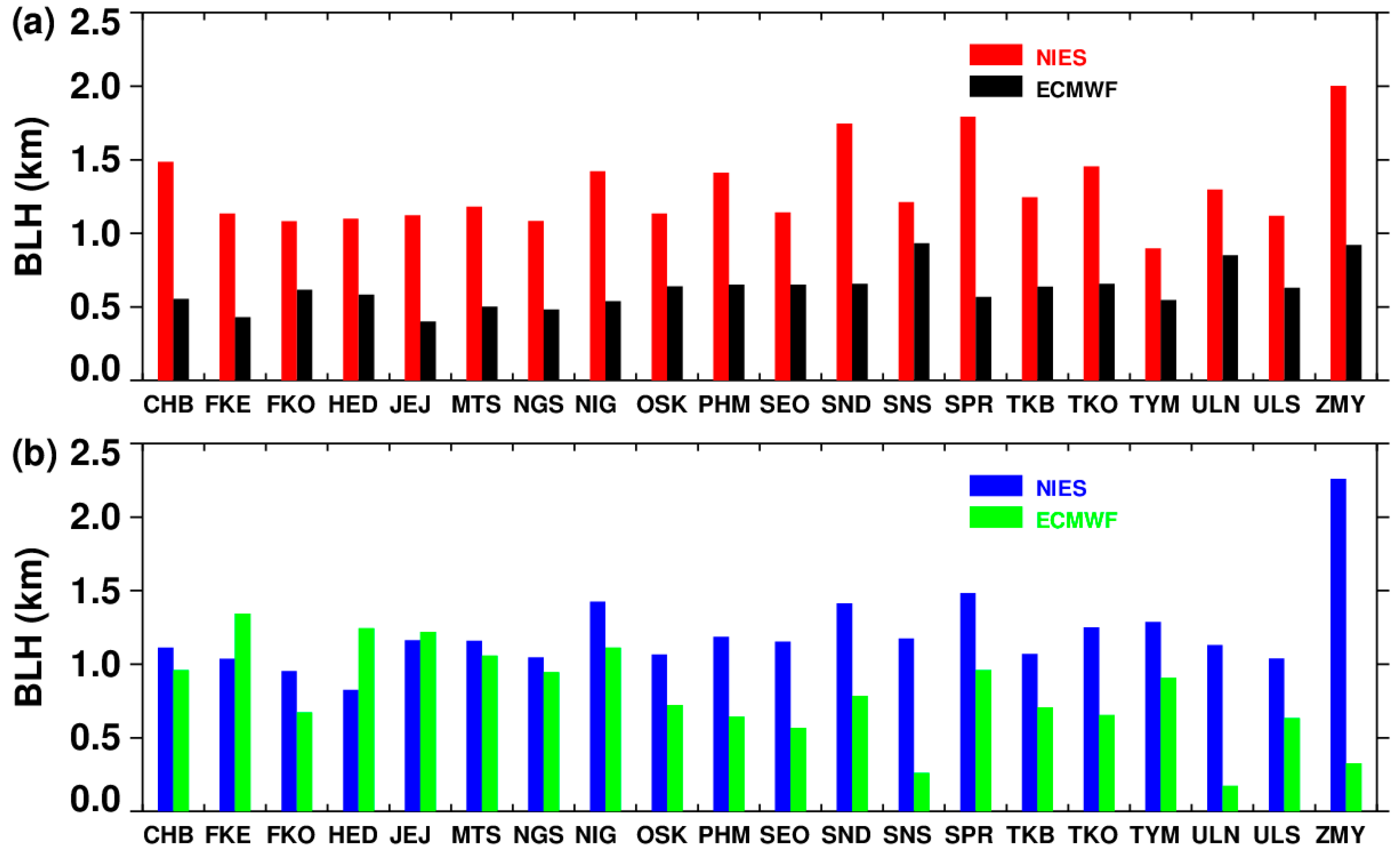
| Summer | Winter | |
|---|---|---|
| Inland | 1.44 | 1.19 |
| Ocean | 1.01 | 1.22 |
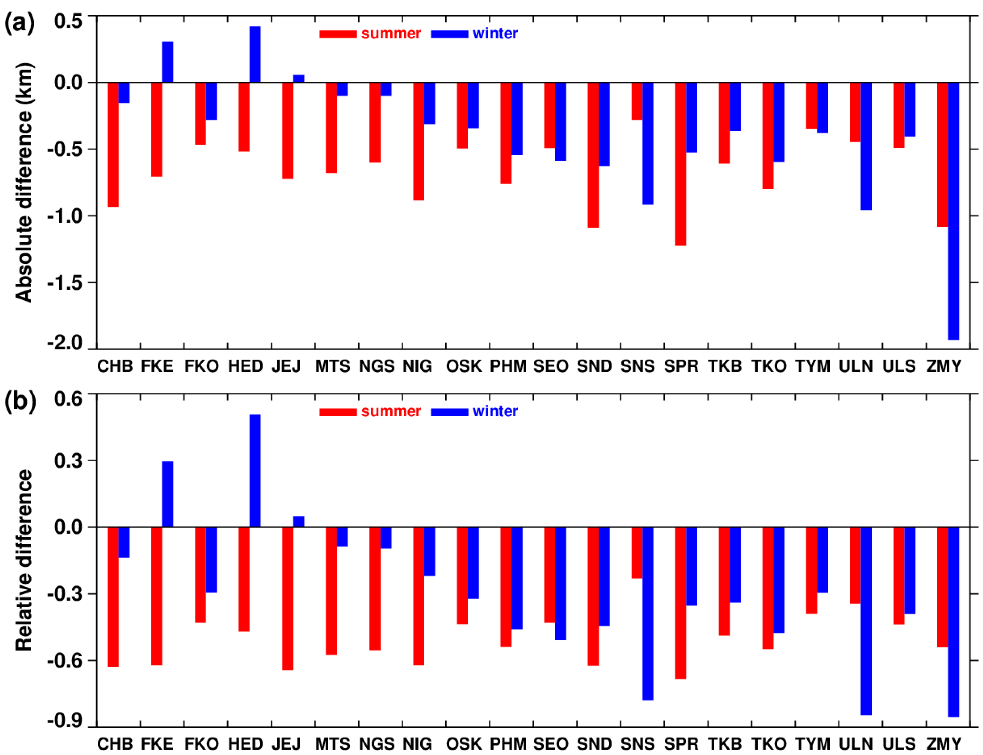
| Absolute Difference (km) | Relative Difference | |||
|---|---|---|---|---|
| Summer | Winter | Summer | Winter | |
| Inland | −0.64 | −1.09 | −0.41 | −0.73 |
| Ocean | −0.65 | 0.26 | −0.58 | 0.28 |
| Coastal areas | −0.70 | −0.37 | −0.53 | −0.30 |
| Mountain | −0.60 | −1.27 | −0.37 | −0.83 |
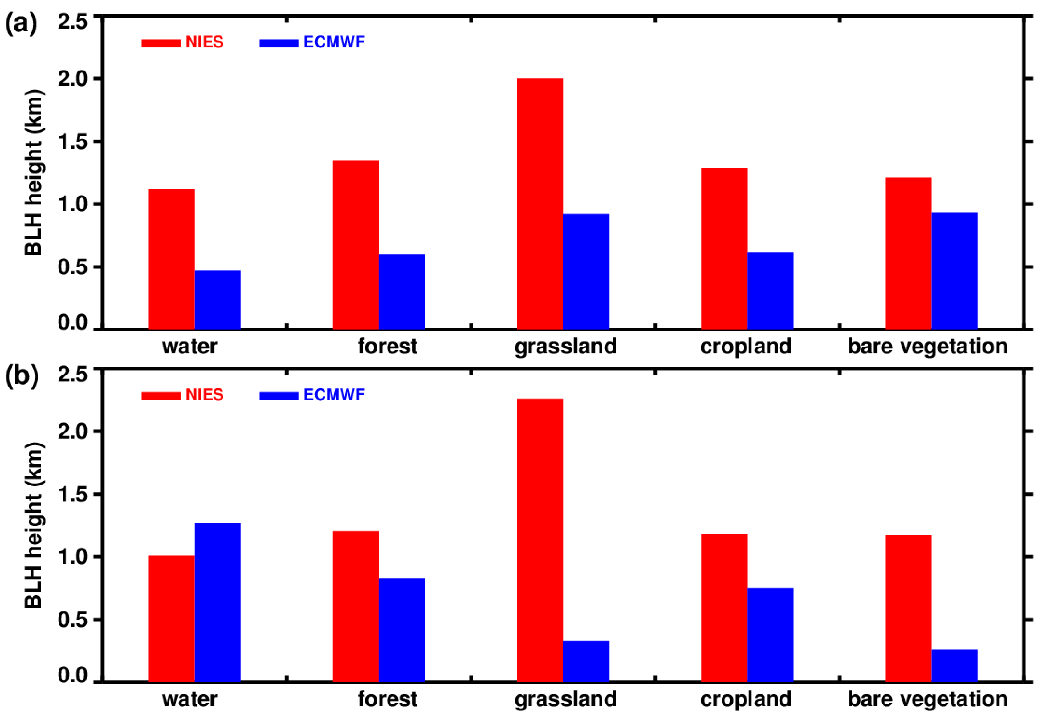
| Water | Forest | Grassland | Cropland | Bare Vegetation | |
|---|---|---|---|---|---|
| Summer | −0.65 | −0.79 | −1.08 | −0.67 | −0.28 |
| Winter | 0.26 | −0.52 | −1.93 | −0.43 | −0.91 |
| Arid | Semi-Arid and Semi-Wet | Wet | |
|---|---|---|---|
| Summer | −0.68 | −0.45 | −0.69 |
| Winter | −1.42 | −0.96 | −0.27 |
Publisher’s Note: MDPI stays neutral with regard to jurisdictional claims in published maps and institutional affiliations. |
© 2022 by the authors. Licensee MDPI, Basel, Switzerland. This article is an open access article distributed under the terms and conditions of the Creative Commons Attribution (CC BY) license (https://creativecommons.org/licenses/by/4.0/).
Share and Cite
Zhang, Z.; Mu, L.; Li, C. Comparison of Planetary Boundary Layer Height Derived from Lidar in AD-Net and ECMWFs Reanalysis Data over East Asia. Atmosphere 2022, 13, 1976. https://doi.org/10.3390/atmos13121976
Zhang Z, Mu L, Li C. Comparison of Planetary Boundary Layer Height Derived from Lidar in AD-Net and ECMWFs Reanalysis Data over East Asia. Atmosphere. 2022; 13(12):1976. https://doi.org/10.3390/atmos13121976
Chicago/Turabian StyleZhang, Zhijuan, Ling Mu, and Chen Li. 2022. "Comparison of Planetary Boundary Layer Height Derived from Lidar in AD-Net and ECMWFs Reanalysis Data over East Asia" Atmosphere 13, no. 12: 1976. https://doi.org/10.3390/atmos13121976