Article

Variations of Secondary PM2.5 in an Urban Area over Central China during 2015–2020 of Air Pollutant Mitigation

1
Key Laboratory for Aerosol-Cloud-Precipitation of China Meteorological Administration, Collaborative Innovation Center on Forecast and Evaluation of Meteorological Disasters, Nanjing University of Information Science and Technology, Nanjing 210044, China
2
Hubei Key Laboratory for Heavy Rain Monitoring and Warning Research, Institute of Heavy Rain, China Meteorological Administration, Wuhan 430205, China
3
Department of Earth and Space Sciences, Southern University of Science and Technology, Shenzhen 518055, China
4
The Institute of Atmospheric Physics, Chinese Academy of Sciences, Beijing 100029, China
*
Author to whom correspondence should be addressed.
Atmosphere 2022, 13(12), 1962; https://doi.org/10.3390/atmos13121962
Submission received: 24 October 2022 / Revised: 9 November 2022 / Accepted: 22 November 2022 / Published: 24 November 2022
(This article belongs to the Special Issue Air Pollution in China (2nd Edition))

Abstract

:
The lack of long-term observational data on secondary PM2.5 (SPM) has limited our comprehensive understanding of atmospheric environment change. This study develops an SPM estimation method, named Single-Tracer Approximate Envelope Algorithm (STAEA), to assess the long-term changes of SPM under different PM2.5 levels and in all seasons in Wuhan, Central China, over the period of anthropogenic pollutant mitigation in 2015–2020. The results show that: (1) the average proportions of SPM in ambient PM2.5 is 59.61% in a clean air environment, rising significantly to 71.60%, 73.73%, and 75.55%, respectively, in light, moderate, and heavy PM2.5 pollution, indicating the dominant role of SPM in air quality deterioration; (2) there are increasing trends of interannual changes of SPM at the light and moderate pollution levels of 1.95 and 3.11 μg·m−3·a−1 with extending SPM proportions in PM2.5 pollution, raising a challenge for further improvement in ambient air quality with mitigating light and moderate PM2.5 pollution; (3) the high SPM contributions ranging from 55.63% to 68.65% on a seasonal average and the large amplitude of seasonal SPM changes could dominate the seasonality of air quality; (4) the wintertime SPM contribution present a consistent increasing trend compared with the declining trends in spring, summer, and autumn, suggesting underlying mechanisms of SPM change for further deciphering the evolution of the atmospheric environment. Our results highlight the effects of air pollutant mitigation on long-term variations in SPM and its contributions with implications for atmospheric environment change.

1. Introduction

Airborne particulate matter (PM) refers to a relatively stable suspension system composed of liquid and solid particles dispersed homogeneously in the atmosphere. Atmospheric fine particles, designated PM2.5, denote the PM with an aerodynamic diameter equal to or less than 2.5μm [1]. A primary cause of air pollution is the high levels of particulate matter, particularly PM2.5 [2]. PM2.5 is composed of both primary PM2.5 (PPM) and secondary PM2.5 (SPM). PPM mainly includes primary organic matter (POA), black carbon (BC), dust, coal smoke, and sea salt directly emitted into the atmosphere by human activities or natural sources [3]. SPM is mainly composed of nitrates, sulfates, ammonium salts, and secondary organics formed by chemical processes involving gaseous precursors SO2, NOx, and volatile organic compounds (VOCs) [1,4]. The PPM and SPM have different effects on air quality and climate systems [5]. For example, the black carbon aerosol is a typical PPM that can strongly absorb solar shortwave radiation, reduce atmospheric visibility, and inhibit the atmospheric radiation balance [6]. In contrast, the S O 4 2 , N O 3 , and N H 4 + in the SPM with a strong optical scatter capacity are also closely correlated with the PH value of atmospheric precipitation [7,8].
Since 2013, China has carried out actions for the prevention and control of PM2.5 pollution (http://www.gov.cn/xinwen/2018-02/01/content_5262720.htm (accessed on 31 August 2022)). As a result, in 2020, the annual mean concentrations of PM2.5 in China fell to 33 μg·m−3 [9]. However, about 80% of the Chinese population is still exposed to annual mean concentrations of PM2.5 exceeding 35 μg·m−3, and 99% of the population is exposed to annual PM2.5 levels over the WHO Air Quality Guidelines of 10 μg·m−3 [10]. On average, during 2014–2018, SPM accounted for 63.5% of the PM2.5 in southern China and 57.1% in northern China [11], suggesting that SPM has become the major part of PM2.5 observed in China. Therefore, the control of PM2.5 pollution in China is confronting a key challenge, owing to our poor understanding of SPM change with a long-term assessment of the contribution to the atmospheric environment [12].
As one of the hub cities in central China, Wuhan has experienced rapid urbanization and modernization, which could potentially exert an impact on air quality [13]. Meanwhile, Wuhan is also located in a key receptor region in the regional transport of air pollutants from the emission source regions in northern China, resulting in heavy PM2.5 pollution in autumn and winter over central China in the urban areas [14,15]. The PM2.5 pollution episodes in Wuhan are characterized by high levels of SIA (secondary inorganic aerosols of sulfate, nitrate, and ammonium) and SOA (secondary organic aerosols) [16]. The sulfur oxidation ratio and nitrogen oxidation ratio are relatively high in winter, and SIAs are the predominant components of wintertime PM2.5 pollution in this urban area [17], indicating the importance of SPM in air pollution and the complexity of changing the urban environment and climate.
Studies on PM2.5 pollution and SPM mainly focus on the Beijing-Tianjin-Hebei region of the North China Plain, the Yangtze River Delta of East China, and the Sichuan Basin of Southwest China. Less attention has been paid to the urban regions in central China. In addition, the SPM is studied using online and offline observation methods to analyze the chemical components and sources of PM2.5. Moreover, most of these SPM studies are restricted to short-term observations with high economic costs and a substantial workforce, making it difficult to conduct long-term studies [18,19,20], which limits our understanding of long-term variations in the SPM with seasonality and its impacts on air quality change. Therefore, the motivation for this study’s targeting of Wuhan, an urban area in central China, is to investigate the multi-year variations in SPM with its contribution to seasonal changes and various levels of air quality over 2015–2020 in the context of reducing anthropogenic pollutant emissions in China. This study aims to assess the variations in SPM over recent-year anthropogenic emission reduction with implications for the importance of secondary aerosols in environmental and climatic changes over urban regions.

2. Data and Methods

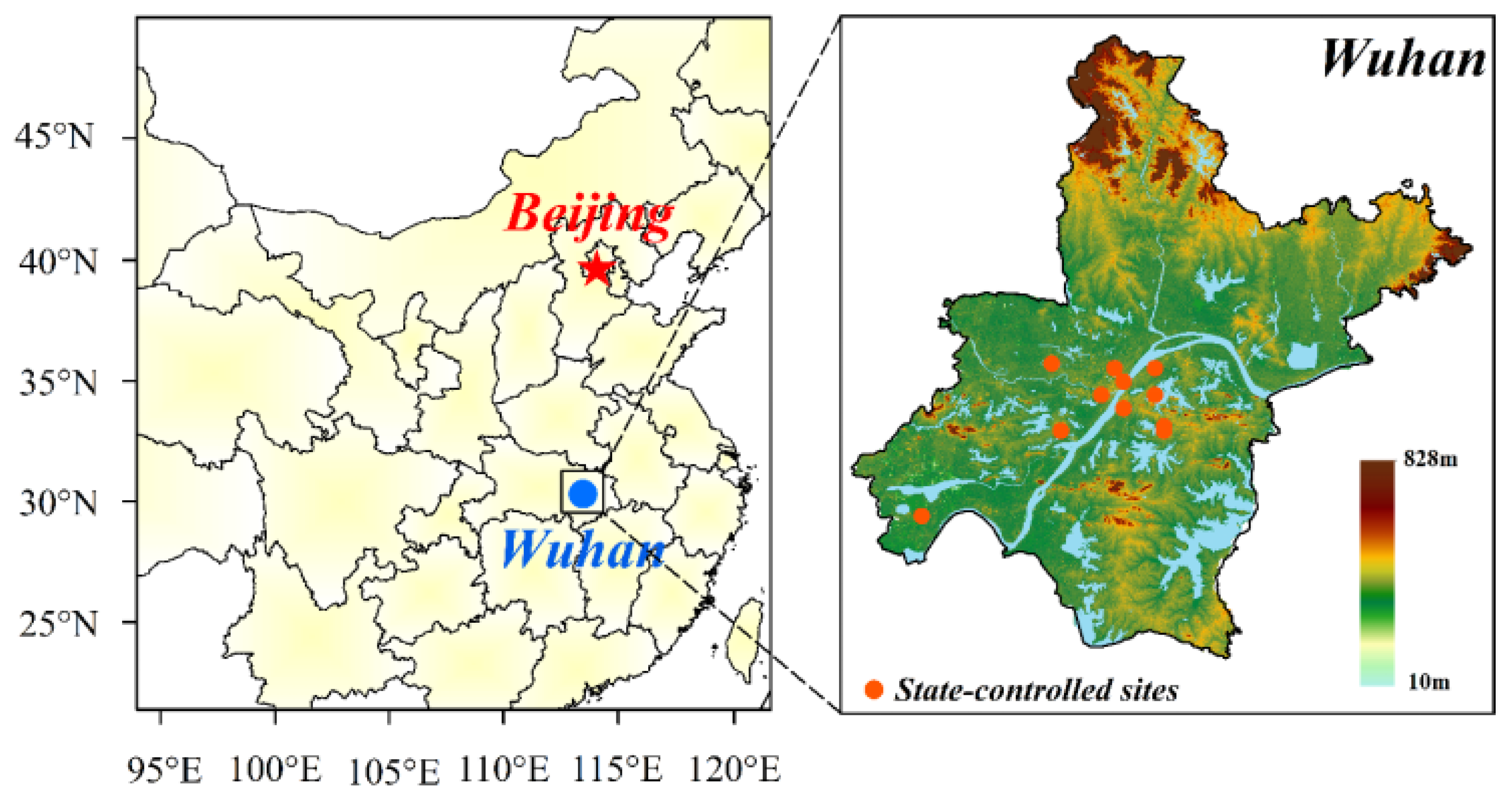
2.1. Environmental and Meteorological Data
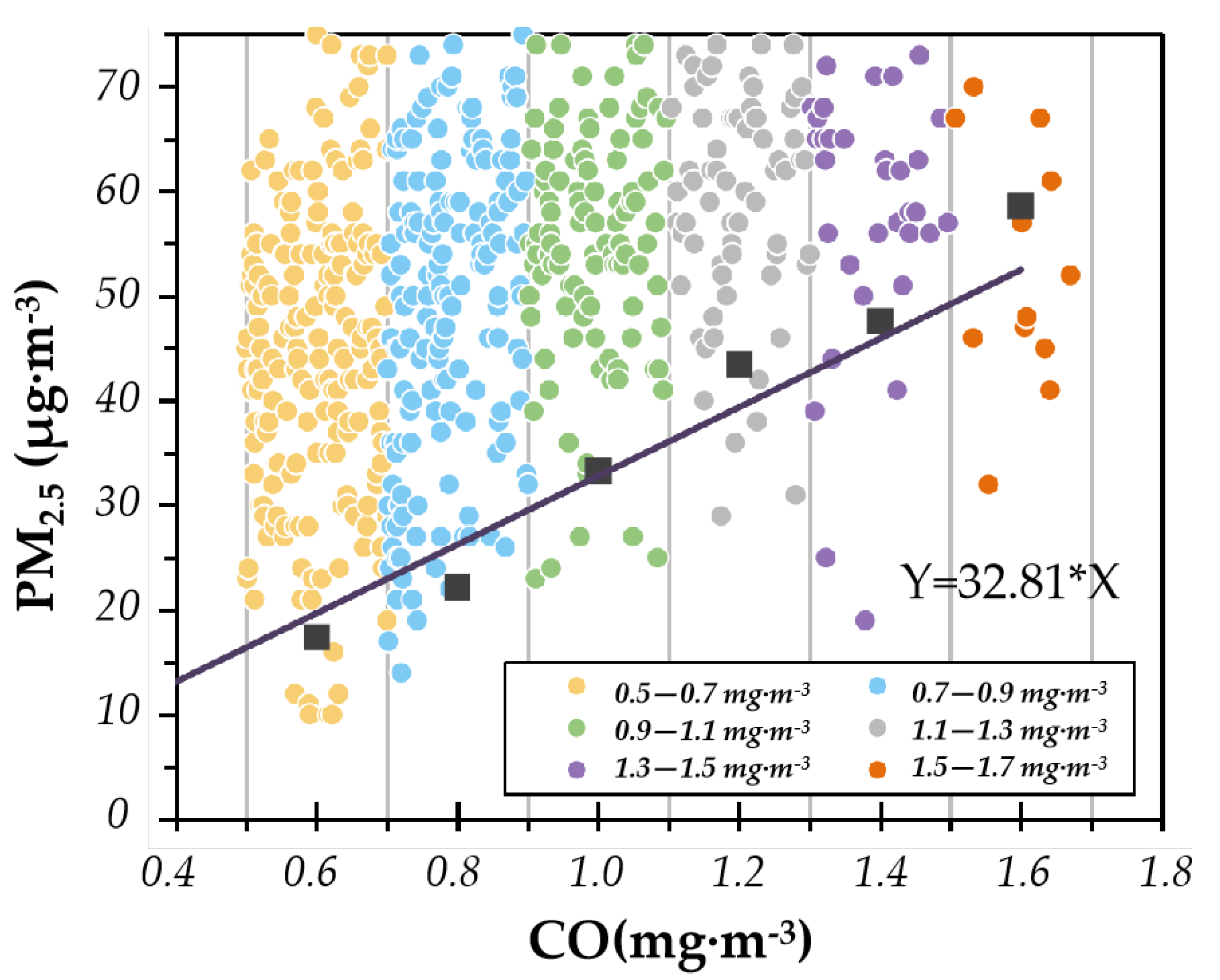
In this study, the monitoring data of air pollutants, including PM2.5, CO, SO2, NO2, and O3 in urban areas of Wuhan (Figure 1) from 1 January 2015 to 31 December 2020, are derived from the China national environmental monitoring network (http://www.mee.gov.cn (accessed on 1 July 2022)), and air pollution data complying with national standards and requirements for ambient air quality monitoring. The urban air pollutant concentrations are represented by the regional averages across the monitoring network in Wuhan. Moreover, meteorological data for air temperature (T), relative humidity (RH), sea level pressure (SLP), wind speed (WS), and wind direction (WD) at the Wuhan observatory of meteorology are sourced from the national meteorological information center of China (http://data.cma.cn/ (accessed on 15 July 2022)), with temporal resolutions of 1 h.
Some unconventional observation data of PM2.5 components, such as water-soluble inorganic ions, organic carbon (OC), and EC, which are derived from continuous online monitoring in urban Wuhan [21,22], with short-term offline sampling at an urban site in Wuhan [23] are used to evaluate the estimated proportion of SPM in PM2.5.

2.2. Methods

Online instrument measurement and offline lab analysis are commonly used to study PM2.5 compositions. These methods can precisely identify the chemical components and source apportionments of PM2.5, which are widely employed in the investigation of secondary particulate matter and its effects on air pollution change [18,19,20,24]. However, these online and offline observation methods can only conduct short-term, single-point studies due to substantial economic costs and huge workforce requirements. Additionally, numerical models, such as the chemical transport model (CTM), are also useful tools for characterizing the secondary PM2.5. Nevertheless, the uncertainties of physical and chemical processes in the CTM and the significant dependence of CTM modeling on air pollutant emissions and meteorological drivers impede the wide use of numerical models to study secondary PM2.5 components [25,26].
Chang and Lee [27] proposed a method for estimating the secondary particles based on the conventional measurements of PM2.5, CO, and O3 with the following considerations: (1) the primary PM2.5 (PPM) is the dominant contributor to ambient PM2.5 under low oxidation capacity with daily maximum O3 concentrations of O3-max < 60 ppb. (2) the ratio of observed PM2.5 and CO under low oxidation capacity (O3-max < 60 ppb), denoted as (PPM/CO)L, is used to represent the fraction of PPM from emission sources, as CO is a typical tracer of primary air pollutants from anthropogenic emissions. (3) The PPM in the light (60 ppb < O3-max < 80 ppb), moderate (80 ppb < O3-max < 120 ppb), and heavy (O3-max > 120 ppb) levels of oxidation capacity can be estimated with the following Equation (1):
PPM = CO × (PPM/CO)L
(4) based on the estimation of PPM from Equation (1), the SPM concentrations and their contribution to ambient PM2.5 (SPMC) are quantitatively estimated with the following equations:
SPM = PM2.5 − PPM
SPMC = SPM/PM2.5
This method of Chang and Lee has been applied widely to assess the secondary particles and their contribution to changes in the atmospheric environment [28,29,30]. However, Gu [31] argued that the contribution of secondary components to PM2.5 cannot be ignored, even in low atmospheric oxidation in the ambient atmosphere, and the weak practicality of Chang and Lee’s methods merely resulted from the uncertainties in (PPM/CO)L, the fraction of PPM from anthropogenic emission sources. Similar to air pollutant change, the uncertainties in (PPM/CO)L are generally decided by meteorological conditions and air pollutant emissions [32]. Therefore, reducing the uncertainties in (PPM/CO)L could improve the method of estimating SPM by considering the influences of meteorological conditions and anthropogenic emissions in the development of the method for this study.

2.3. Development of Method

In this study, the (PPM/CO)L ratio (Equation (1)) is defined as RPPM/CO, and we develop a more accurate estimation method for SPM concentration, named the Single-Tracer Approximate Envelope Algorithm (STAEA) based on the AEM method [29], first of the AEM without comprehensively considering the influences of meteorological conditions on RPPM/CO estimation. For instance, wet deposition of the precipitation process can remove PM2.5 but not insoluble CO, which would lead to a significant underestimation of the RPPM/CO ratio. Furthermore, in order to possibly minimize the concentrations of SPM in observed PM2.5 with accurate estimations of RPPM/CO, the AEM method discusses the SPM concentration changes in different air quality levels while not involving the impacts of atmospheric oxidation on the formation of secondary aerosols [33]. Therefore, the STAEA-method filter through the observed PM2.5 and CO data for clean air quality (daily mean PM2.5 concentration < 75 μg·m−3), low photochemical activities (maximum hourly concentration O3-max < 60 ppb), and non-precipitation days (daily precipitation amount = 0.0 mm), aims to reduce the uncertainties in RPPM/CO from meteorological conditions.
Another major improvement over the AEM method is that STAEA estimation can possibly eliminate the impact of anthropogenic emission changes. (1) RPPM/CO ratios vary along with significant changes in the anthropogenic emissions of different seasons over the recent-year mitigation and different times of day. Therefore, separately estimating RPPM/CO for different time periods can reduce the uncertainties from emission changes. (2) The STAEA method is based on an essential presumption that the air pollutant source emissions in a certain area remained stable during a short time period, which means that the estimated PPM/CO ratios should remain unchanged regardless of high or low CO levels.
Our estimations of RPPM/CO divided one day into 8 time periods to respectively estimate 192 different RPPM/CO (6 years × 4 seasons × 8 time-periods) from 2015 to 2020, and each 3-h period of PM2.5 with its corresponding CO concentrations was grouped according to the CO concentration bins with the ranges over 0.5–0.7, 0.7–0.9, 0.9–1.1, 1.1–1.3, 1.3–1.5, and 1.5–1.7 mg·m−3 [29]. For the sake of estimating RPPM/CO with the minimum possible impact of SPM, the lowest ψ (ψ = 1, 2, 3, …) numbers of PM2.5 concentrations within CO bins with a corresponding CO level were averaged to represent estimated RPPM/CO ratios (black squares, Figure 2), and the robust RPPM/CO is the slope of the fitting line for black squares with an optimal fitting degree.

2.4. STAEA Method Evaluation

To assess the improvement of the STAEA-estimated contribution of SPM to PM2.5, we compared the errors of STAEA and AEM estimations with observation-based analyses of PM2.5 components from published studies (Table 1). The secondary organic carbon (SOC) concentrations could usually be estimated by the elemental carbon (EC)-tracer method [34], and the secondary organic aerosol (SOA) concentrations were calculated by multiplying the SOC concentration by an empirical coefficient of 2.0 [35], with the following steps:
SOC = OC − EC × (OC/EC)min
SOA = 2.0 × SOC
where OC denotes the mass concentrations of organic carbon and (OC/EC)min represents the minimum observed OC/EC in primary emissions. The concentrations of secondary inorganic aerosol (SIA) were estimated using the accumulation of water-soluble inorganic ions (WSIIs), such as sulfate, nitrate, and ammonium concentrations. As SPM is the sum of SIA and SOA, the ratio of SPM/PM2.5 could be estimated with the concentrations of PM2.5 and SPM (Table 1).
The evaluation of STAEA estimations presents the reasonable performances of SPM concentrations and the contribution rate of SPM/PM2.5 based on the comparisons with the available measurements (Table 1). Furthermore, averaged over three measurement periods, the STAEA estimation error of 9.06% is much lower than the AEM estimation with a mean error of 29.71%, confirming a significant improvement of secondary PM2.5 estimation with our developed STAEA method. However, there were discrepancies between the estimations and the measurements of secondary PM2.5, which could have resulted from the STAEA estimations considering only anthropogenic emissions with a CO tracer and excluding the natural emissions of PM2.5, as well as the different sampling sites and observation periods. Overall, the STAEA estimation could better capture the changes in secondary PM2.5 concentrations with the contributions to ambient PM2.5, which could be used in the following analysis of variations in secondary PM2.5 in Wuhan over the 2015–2020 period of emission reduction.

3. Results and Discussion

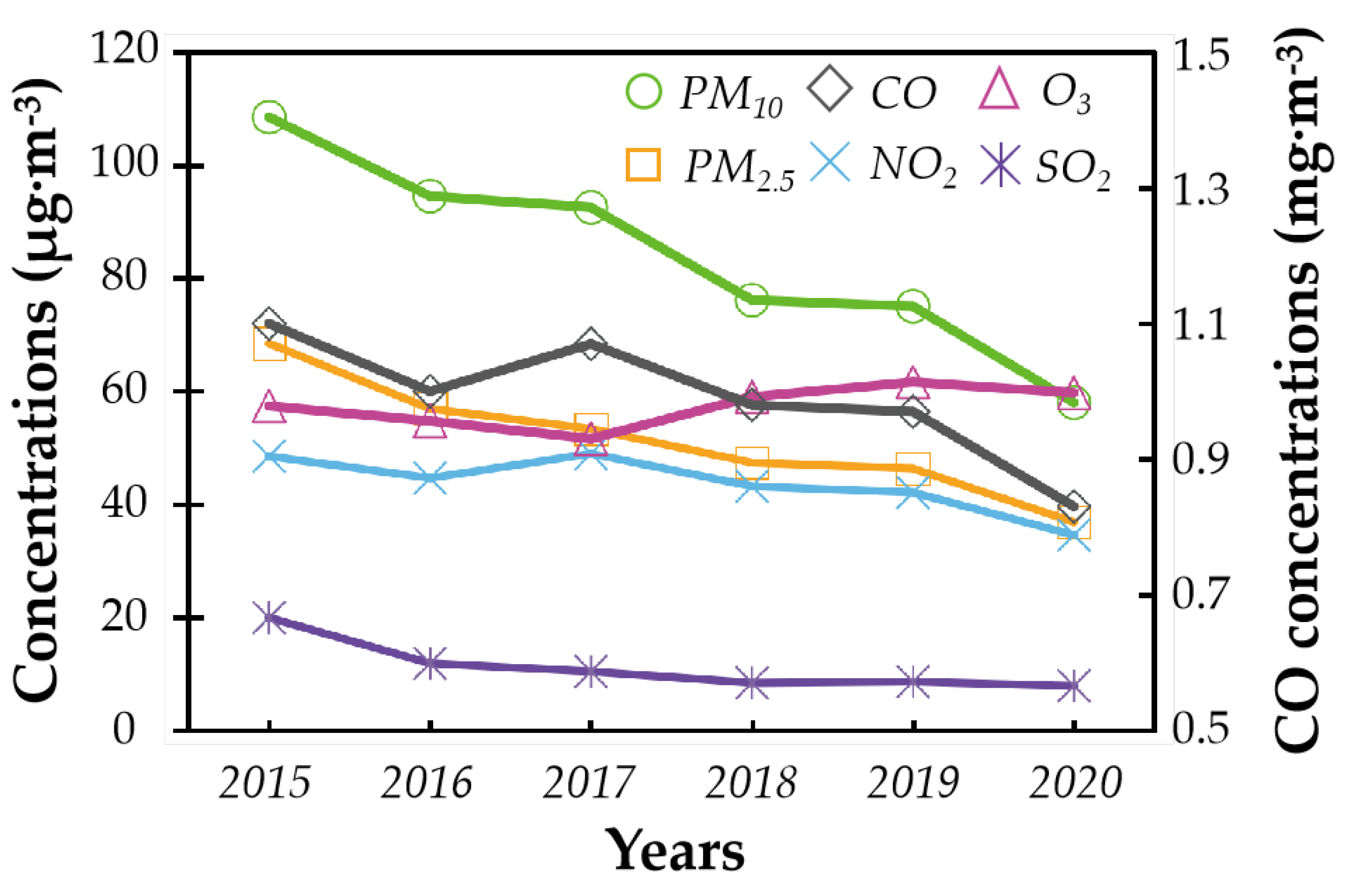
3.1. Variations of Air Pollutants and PM2.5 Pollution

The interannual variations in ambient air pollutants in Wuhan over 2015–2020 are shown in Figure 3, based on the data from the air quality monitoring network. The annual averages of PM2.5 concentrations dropped from 68.49 μg·m−3 in 2015 to 36.84 μg·m−3 in 2020 in Wuhan, presenting a significant decrease of 46.21% with air pollutant emission control in China over the 2015–2020 period. Similarly, the annual averages of PM10 concentrations fell by 46.57% from 108.56 μg·m−3 in 2015 to 58.00 μg·m−3 in 2020. In addition, the annual mean concentrations of the gaseous pollutants NO2, SO2, and CO were 34.55 μg·m−3, 7.84 μg·m−3, and 0.83μg·m−3 in 2020, respectively, a decrease of 30.20%, 60.64%, and 24.55% compared with 2015, demonstrating that the urban area in central China had achieved a remarkable improvement in air quality with the past 6-year anthropogenic pollutant mitigation period. However, the annual mean of near-surface O3 concentrations exhibited an increase from 57.40 μg·m−3 in 2015 to 59.74 μg·m−3 in 2020, indicating the potential enhancement of oxidation capacity in the ambient atmosphere during air pollutant mitigation during 2015–2020.
Based on the daily PM2.5 concentration ranges over 0–75 μg·m−3, 75–115 μg·m−3, 115–150 μg·m−3, and higher than 150 μg·m−3, ambient environment was classified respectively into clean air qualities of light, moderate and heavy PM2.5 pollution according to the national standard of ambient air quality in China (Ministry of Ecology and Environment of China, available at: https://www.mee.gov.cn/ (accessed on 31 August 2022)). With this classification of air quality levels, it was found in Wuhan that during 2015–2020 the annual number of days with clean air quality increased from 240 days in 2015 to 340 days in 2020, and light (moderate) PM2.5 pollution days decreased from 76 (31) days in 2015 to 23 (3) days in 2020 (Table 2). Noticeably, heavy PM2.5 pollution days dropped from 17 days in 2015 to 0 days in 2020, with heavy PM2.5 pollution eliminated in 2020 (Table 2).
The combined effects of local accumulation, regional transport, and secondary aerosol formation show great seasonal changes in atmospheric pollution in urban areas [14,36,37]. Winter is a typical season with frequent PM2.5 pollution in Wuhan. As listed in Table 3, the 6-year period (2015–2020) had a cumulative 285 days with PM2.5 pollution in winter, which was much more than 68, 61, and 2 days in spring, autumn, and summer, respectively. Wintertime accounted for 68.51% of PM2.5 pollution days over the past 6 years. Taking 2015–2020 as a whole, light, moderate, and heavy PM2.5 pollution days in Wuhan accounted for 69.47%, 20.91%, and 9.62% of all PM2.5 pollution days, respectively, with a ratio of about 7:2:1 among light, moderate, and heavy levels of PM2.5 pollution. Therefore, the light level of PM2.5 pollution was the dominant urban PM2.5 pollution in all seasons, and the occurrence peaks were seen in winter.
In summary, Wuhan has been experiencing significant decreases in PM2.5, PM10, CO, SO2, and NO2 levels since 2013, reflecting the great effects of stringent emission control on air quality improvement. However, the near-surface O3 exhibited an increasing trend with the dominance of light PM2.5 pollution in urban air pollution over the recent-year air pollutant mitigation, implying the importance of atmospheric oxidation for SPM in light air pollution. The long-term variations in SPM over recent years of anthropogenic emission mitigation remain unclear in the urban region, limiting our understanding of air quality evolution with implications for further fine control of air pollution and atmospheric environment management.

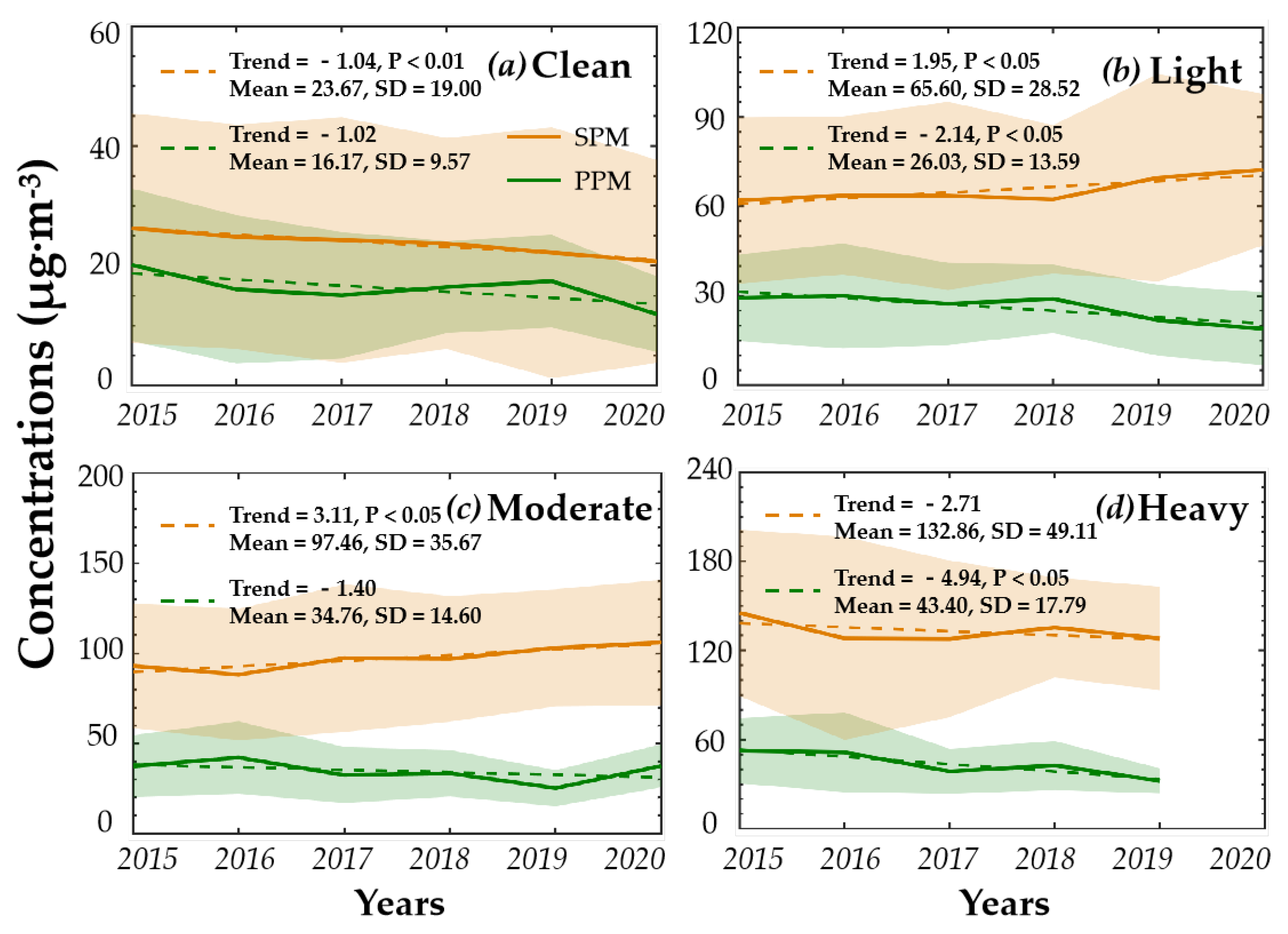
3.2. Long-Term Variations of SPM in Air Quality Levels

Long-term variations in the SPM influencing air quality are important for understanding the changes in the atmospheric environment and assessing the emission control for mitigating air pollution. Therefore, we employed the STAEA method here to estimate the changes in SPM and PPM in Air Quality Levels with the various levels of ambient PM2.5 based on the 6-year (2015–2020) data from meteorological and environmental observations in the urban Wuhan region of central China.
Based on the STAEA estimations, Figure 4 presents the interannual variations in SPM and PPM with the linear trends, average values, and standard deviations in different PM2.5 levels over 2015–2020. With a deterioration in the urban air quality from clean air quality, light, moderate to heavy PM2.5 pollution, the recent-year averages of SPM concentrations increased from 23.67 μg·m−3, 65.60 μg·m−3, 97.46 μg·m−3 to 132.86 μg·m−3 accompanied by PPM concentrations aggravating ambient PM2.5 levels (Figure 4). With the ratio of SPM/PM2.5 representing the contribution of SPM to the ambient PM2.5 concentration, the urban air quality changes in Wuhan over 2015–2020 are reckoned to be the results of contributions of SPM to different PM2.5 levels enhanced from 59.61% in clean air quality to 71.60%, 73.73%, and 75.55%, respectively in light, moderate, and heavy PM2.5 pollution, indicating that SPM has become a dominant component of PM2.5 deteriorating the urban environment. The mitigation of secondary aerosol formation could largely improve air quality.
Accompanying decreasing PPM concentrations between 2015 and 2020, the annual concentrations of SPM in clean air quality decreased from 26.29 μg·m−3 in 2015 to 20.71 μg·m−3 in 2020, while there were contrasting patterns of interannual SPM changes at the light and moderate pollution levels with annual concentrations of SPM increasing, respectively, from 62.01 μg·m−3 and 93.11 μg·m−3 in 2015 to 72.30 μg·m−3 and 106.04 μg·m−3 in 2020 (Figure 4). These results highlight a distinctly important role for SPM in light and moderate air pollution over the recent years of anthropogenic pollutant mitigation. Furthermore, heavy PM2.5 pollution was eliminated in 2020 as both PPM and SPM concentrations in heavy air pollution fell significantly from 2015 to 2020. To statistically detect the long-term variations in SPM contributions to ambient PM2.5 levels, the difference (DF) between the linear trends of SPM (TrendS) and PPM (TrendP) over recent years is introduced here as follows:
DF = TrendS − TrendP
with a positive (negative) DF representing the increasing (decreasing) contribution of SPM to ambient PM2.5 concentration in long-term changes in the atmospheric environment.
As shown in Figure 4 and Table 4, the PPM concentrations exhibited decreasing trends in clean air quality and all air pollution levels over 2015–2020, with the most prominent trend (−4.94 μg·m−3·a−1) in heavy air pollution, reflecting the consistent declines in PPM in air quality change over the recent years of anthropogenic pollutant emission reduction. The long-term change trends of SPM in the atmospheric environment are noteworthy, with the negative linear trends at −1.04 μg·m−3·a−1 in a clean air environment and at −2.71 μg·m−3·a−1 in heavy PM2.5 pollution, in contrast with the positive trends at 1.95 μg·m−3·a−1 and 3.11 μg·m−3·a−1 in light and moderate pollution, respectively (Figure 4; Table 4). By comparing the DF values at different air quality levels (Table 4), clean air quality uniquely has a descending contribution of SPM (DF = −0.02 μg·m−3·a−1) over the recent years, differing from the increasing contributions of secondary aerosols to PM2.5 pollution change over the emission control process [38,39]. Furthermore, the contributions of SPM to light and moderate PM2.5 pollution, as indicated respectively with the high DF values of 4.09 and 4.51 (Table 4), were largely intensified in this urban area during 2015–2020, confirming the difficulty of improving air quality with the enhancement trends in secondary aerosols with high contributions to light and moderate PM2.5 pollution during recent years of PPM reductions [40].
Standard deviation, as a statistical measure of dispersion in a frequency distribution, is used to characterize the amplitude of SPM and PPM in long-term variations in an atmospheric environment. Comparing the standard deviations (SD) of PPM and SPM over 2015–2020 (Figure 4), it is remarkable that the SD values of SPM are more than 2 times greater than the PPM changes for all the ambient PM2.5 levels from clean air quality, light, moderate, and heavy air pollution, presenting the significantly large extent of SPM in air quality change. These values could have resulted from the complex physical and chemical processes of secondary aerosols with more influence factors than primary aerosols. The large amplitude of SPM variations with the more complex mechanism could raise the difficulty of air quality management, and it is more feasible to improve the atmospheric environment using fine control of the secondary aerosols.

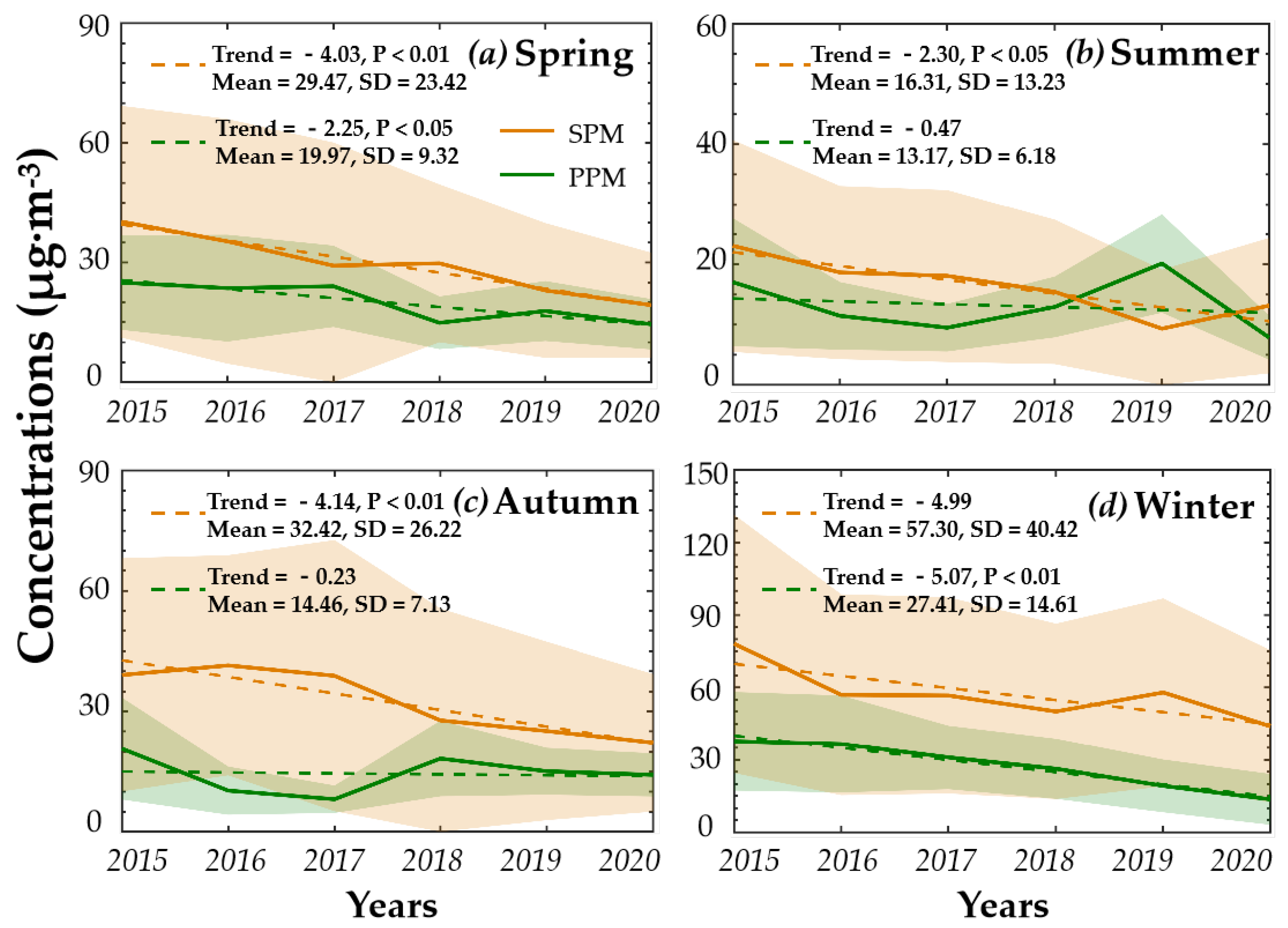
3.3. Seasonal Variations of SPM and PPM

The seasonal changes in secondary particles with their contributions to ambient PM2.5 are attributed to the variations in air pollutant emissions related to human activities as well as the meteorological conditions affecting the atmospheric processes of chemistry and physics. In this section, the STAEA estimations are used to identify the seasonal changes in SPM and PPM to further understand the urban environment of central China in Wuhan.
Based on the STAEA estimations over 2015–2020 (Figure 5), the seasonal mean SPM and PPM concentrations reached up to 57.30 μg·m−3 and 27.41 μg·m−3 in winter, and fell to 16.31 μg·m−3 and 13.17 μg·m−3 in summer, presenting the seasonal oscillations of both PPM and SPM between the highest levels in winter and the lowest levels in summer. The seasonal contributions of SPM to the PM2.5 levels were averaged at 55.63% in summer, while the high contributions of SPM were 68.65% and 68.33% in autumn and winter, respectively. Such results are in accordance with previous studies [11]. High levels of SPM could largely contribute to poor air quality in winter with frequent PM2.5 pollution (Table 3).
As presented in Figure 5 and Table 5, both SPM and PPM concentrations exhibited decreasing trends in all seasons over 2015–2020, with the most significant declines of −4.99 μg·m−3·a−1 and −5.07 μg·m−3·a−1, respectively, for SPM and PPM in winter. The seasonality of SPM contributions in the changes of atmospheric environment is noteworthy, with a positive DF (Equation (6)) value at 0.08 μg·m−3·a−1 in winter and negative DF values of −1.78 μg·m−3·a−1, −1.83 μg·m−3·a−1, and −3.91 μg·m−3·a−1 in spring, summer, and autumn (Table 5). The SPM contribution to the wintertime high PM2.5 levels was enhanced from year to year, accompanied by the descending trends in SPM and PPM over the 2015–2020 period of anthropogenic emission reduction (Figure 5; Table 5), which is consistent with our current understanding of atmospheric environmental change [11,38]. However, it is puzzling that the contributions of SPM to ambient PM2.5 declined in spring, summer, and autumn in contrast with wintertime’s increasing SPM contribution over the recent-year air pollution controls. Such an increase could imply the potential mechanisms of SPM change for further study in understanding atmospheric environment change with the thresholds of reducing air pollutant emissions to mitigate SPM potency for effectively improving air quality.
Furthermore, the SD values of SPM are identified as larger than the PPM changes in all seasons, comparing the standard deviations (SD) of PPM and SPM over 2015–2020 (Figure 5). The large amplitude of seasonal SPM variations could dominate the seasonality of urban air quality for air environment management.

4. Conclusions

Previous studies of secondary aerosols were limited to observation-based analyses of short-term PM2.5 components with PM2.5 pollution episodes, leading to our poor understanding of long-term SPM change and its contribution to the atmospheric environment. In this study, we developed the SPM estimation method (STAEA) based on routine environmental and meteorological monitoring data. Compared with the existing AEM estimations and measurements, the STAEA method was confirmed to have a better performance in capturing the SPM concentrations and their contributions to ambient PM2.5. We employed the STAEA method to investigate the 6-year changes of SPM and its contributions to seasonal variations and changing levels of air quality in Wuhan during the 2015–2020 mitigation of anthropogenic air pollutants. The major conclusions are highlighted as follows:
The contributions of SPM to ambient PM2.5 levels increase from 59.61% in clean air quality to 71.60%, 73.73%, and 75.55%, respectively, in light, moderate, and heavy PM2.5 pollution levels, with the key components of PM2.5 in a deteriorating atmospheric environment over 2015–2020. The long-term changes in light and moderate PM2.5 pollution with increasing SPM trends at 1.95 and 3.11 μg·m−3·a−1 and the enhancement of the SPM contributions to PM2.5 pollution could aggravate difficulties in the improvement of the atmospheric environment. Both PPM and SPM oscillate seasonally between high levels in winter and low levels in summer, and the large amplitude of seasonal SPM variations could dominate the seasonality of urban air quality. The contributions of SPM to seasonal PM2.5 changes declined in spring, summer, and autumn in contrast with a wintertime increase in the SPM contribution to frequent air pollution. The SPM contributions to the atmospheric environment rise in winter with the descending trends of SPM and PPM at all seasons over 2015–2020, implying the potential mechanisms of SPM change for further understanding atmospheric environment change.
The present study investigates the variations of secondary PM2.5 in an urban area over central China during 2015–2020 with the continuous emission control since 2013 and the unexpected reduction of anthropogenic emissions attributed to the COVID-19 lockdowns. Due to a limited understanding of the complex mechanisms of secondary aerosol formation, further research could be desired with more comprehensive, longer, and updated observations and simulation analyses of atmospheric chemical and physical processes to generalize the regional changes in secondary aerosols and their implications for the multi-scale changes in the atmospheric environment and the improvement of air quality.

Author Contributions

Conceptualization and methodology, D.L. and T.Z.; software and visualization, D.L., Y.W., and Z.L.; observational data, Y.B. and Y.Z. (Yan Zhu); writing—original draft preparation, D.L. and Y.Z. (Yan Zhu); writing—review and editing, T.Z. and D.L; formal analysis and discussion, D.L., T.Z., Y.Z. (Yan Zhu), W.F. and Y.Z. (Yuqing Zhang). All authors have read and agreed to the published version of the manuscript.

Funding

This research was funded by the National Science Foundation of China (Grant No. 41830965, 42075186, and 42275196) and the National Key Research and Development Program of China (Grant No. 2022YFC3701204).

Institutional Review Board Statement

Not applicable.

Informed Consent Statement

Not applicable.

Data Availability Statement

Not applicable.

Acknowledgments

Special thanks to T.Z. for his patient instruction and meticulous review.

Conflicts of Interest

The authors declare no conflict of interest.

References

  1. Zhang, R.; Wang, G. Formation of urban fine particulate matter. Chem. Rev. 2015, 115, 3803–3855. [Google Scholar] [CrossRef]
  2. Guo, S.; Hu, M. Elucidating severe urban haze formation in China. Proc. Natl. Acad. Sci. USA 2014, 111, 17373–17378. [Google Scholar] [CrossRef] [Green Version]
  3. Hu, M.; Guo, S. Insight into characteristics and sources of PM2.5 in the Beijing–Tianjin–Hebei region, China. Natl. Sci. Rev. 2015, 2, 257–258. [Google Scholar] [CrossRef]
  4. Huang, R.; Zhang, Y. High secondary aerosol contribution to particulate pollution during haze events in China. Nature 2014, 514, 218–222. [Google Scholar] [CrossRef] [Green Version]
  5. Li, K.; Jacob, D.J. A two-pollutant strategy for improving ozone and particulate air quality in China. Nat. Geosci. 2019, 12, 906–910. [Google Scholar] [CrossRef]
  6. Yang, X.; Huang, Y. Influence of fine particulate matter on atmospheric visibility. Chin. Sci. Bull. 2013, 58, 1165–1170. [Google Scholar] [CrossRef]
  7. Kerminen, V.M.; Hillamo, R. Ion balances of size-resolved tropospheric aerosol samples: Implications for the acidity and atmospheric processing of aerosols. Atmos. Environ. 2001, 35, 5255–5265. [Google Scholar] [CrossRef]
  8. Yao, X.; Fang, M. The size dependence of chloride depletion in fine and coarse sea-salt particles. Atmos. Environ. 2003, 37, 743–751. [Google Scholar] [CrossRef]
  9. Zhang, Q.; Geng, G. Impact of clean air action on PM2.5 pollution in China. Sci. China Earth Sci. 2019, 62, 1845–1846. [Google Scholar] [CrossRef] [Green Version]
  10. Wang, Q.; Wang, J. Estimation of PM2.5-associated disease burden in China in 2020 and 2030 using population and air quality scenarios: A modelling study. Lancet Planet. Health 2019, 3, 71–80. [Google Scholar] [CrossRef]
  11. Zhang, H.; Li, N. Estimation of secondary PM2.5 in China and the United States using a multi-tracer approach. Atmos. Chem. Phys. 2022, 22, 5495–5514. [Google Scholar] [CrossRef]
  12. Zhang, Y.; Jin, J. Long-term variations of major atmospheric compositions observed at the background stations in three key areas of China. Adv. Clim. Chang. Res. 2020, 11, 370–380. [Google Scholar] [CrossRef]
  13. Molina, L.T. Introductory lecture: Air quality in megacities. Faraday Discuss. 2021, 226, 9–52. [Google Scholar] [CrossRef] [PubMed]
  14. Bai, Y.; Zhao, T. Meteorological mechanism of regional PM2.5 transport building a receptor region for heavy air pollution over Central China. Sci. Total Environ. 2022, 808, 151951. [Google Scholar] [CrossRef]
  15. Shen, L.; Zhao, T. Importance of meteorology in air pollution events during the city lockdown for COVID-19 in Hubei Province, Central China. Sci. Total Environ. 2021, 754, 142227. [Google Scholar] [CrossRef] [PubMed]
  16. Wang, G.; Zhang, R. Persistent sulfate formation from London Fog to Chinese haze. Proc. Natl. Acad. Sci. USA 2016, 113, 13630–13635. [Google Scholar] [CrossRef] [PubMed] [Green Version]
  17. Mu, L.; Zheng, L. Characterization and Source Analysis of Water-soluble Ions in Atmospheric Particles in Jinzhong, China. Aerosol Air Qual. Res. 2019, 19, 2394–2409. [Google Scholar] [CrossRef]
  18. Gao, J.; Wang, K. Temporal-spatial characteristics and source apportionment of PM2.5 as well as its associated chemical species in the Beijing-Tianjin-Hebei region of China. Environ. Pollut. 2018, 233, 714–724. [Google Scholar] [CrossRef] [PubMed]
  19. Xu, H.; Xiao, Z. Spatial and temporal distribution, chemical characteristics, and sources of ambient particulate matter in the Beijing-Tianjin-Hebei region. Sci. Total Environ. 2019, 658, 280–293. [Google Scholar] [CrossRef]
  20. Wang, H.; Tian, M. Seasonal characteristics, formation mechanisms and source origins of PM2.5 in two megacities in Sichuan Basin, China. Atmos. Chem. Phys. 2018, 18, 865–881. [Google Scholar] [CrossRef]
  21. Huang, F.; Zhou, J. Chemical characteristics and source apportionment of PM2.5 in Wuhan, China. J. Atmos. Chem. 2019, 76, 245–262. [Google Scholar] [CrossRef]
  22. Zheng, H.; Kong, S. Significant changes in the chemical compositions and sources of PM2.5 in Wuhan since the city lockdown as COVID-19. Sci. Total Environ. 2020, 739, 140000. [Google Scholar] [CrossRef] [PubMed]
  23. Chen, D.; Zhang, Z. Analysis of PM2.5 Oxidative Potential during a Period of Heavy Pollution in Winter, Wuhan. Environ. Sci. Technol. 2020, 43, 171–176. (In Chinese) [Google Scholar] [CrossRef]
  24. Dai, Q.; Bi, X. Chemical nature of PM2.5 and PM10 in Xi’an, China: Insights into primary emissions and secondary particle formation. Environ. Pollut. 2018, 240, 155–166. [Google Scholar] [CrossRef] [PubMed]
  25. Chen, X.; Yang, T. Investigating the impacts of coal-fired power plants on ambient PM2.5 by a combination of a chemical transport model and receptor model. Sci. Total Environ. 2020, 727, 138407. [Google Scholar] [CrossRef]
  26. Štefánik, D.; Matejovičová, J. Comparison of two methods of calculating NO2 and PM10 transboundary pollution by CMAQ chemical transport model and the assessment of the non-linearity effect. Atmos. Pollut. Res. 2020, 11, 12–23. [Google Scholar] [CrossRef]
  27. Chang, S.; Lee, C. Secondary aerosol formation through photochemical reactions estimated by using air quality monitoring data in Taipei City from 1994 to 2003. Atmos. Environ. 2007, 41, 4002–4017. [Google Scholar] [CrossRef]
  28. Jia, M.; Zhao, T. Inverse Relations of PM2.5 and O3 in Air Compound Pollution between Cold and Hot Seasons over an Urban Area of East China. Atmosphere 2017, 8, 59. [Google Scholar] [CrossRef] [Green Version]
  29. Du, X.; Shi, G. Contribution of Secondary Particles to Wintertime PM2.5 During 2015–2018 in a Major Urban Area of the Sichuan Basin, Southwest China. Earth Space Sci. 2020, 7, e2020EA001194. [Google Scholar] [CrossRef]
  30. Luo, Y.; Zhao, T. Seasonal changes in the recent decline of combined high PM2.5 and O3 pollution and associated chemical and meteorological drivers in the Beijing–Tianjin–Hebei region, China. Sci. Total Environ. 2022, 838, 156312. [Google Scholar] [CrossRef]
  31. Gu, J.; Chen, Z. Characterization of Atmospheric Fine Particles and Secondary Aerosol Estimated under the Different Photochemical Activities in Summertime Tianjin, China. Int. J. Environ. Res. Public Health 2022, 19, 7956. [Google Scholar] [CrossRef]
  32. Rahman, M.M.; Shuo, W. Investigating the Relationship between Air Pollutants and Meteorological Parameters Using Satellite Data over Bangladesh. Remote Sens. 2022, 14, 2757. [Google Scholar] [CrossRef]
  33. Na, K.; Sawant, A.A. Primary and secondary carbonaceous species in the atmosphere of Western Riverside County, California. Atmos. Environ. 2004, 38, 1345–1355. [Google Scholar] [CrossRef]
  34. Castro, L.M.; Pio, C.A. Carbonaceous aerosol in urban and rural European atmospheres: Estimation of secondary organic carbon concentrations. Atmos. Environ. 1999, 33, 2771–2781. [Google Scholar] [CrossRef]
  35. Yin, C.; Wang, T. Assessment of direct radiative forcing due to secondary organic aerosol over China with a regional climate model. Tellus B Chem. Phys. Meteorol. 2015, 67, 24634. [Google Scholar] [CrossRef] [Green Version]
  36. Zhao, H.; Gui, K. Effects of Different Aerosols on the Air Pollution and Their Relationship With Meteorological Parameters in North China Plain. Front. Environ. Sci. 2022, 10, 814736. [Google Scholar] [CrossRef]
  37. Xu, Z.; Liu, Z. Classification of Urban Pollution Levels Based on Clustering and Spatial Statistics. Atmosphere 2022, 13, 494. [Google Scholar] [CrossRef]
  38. Huang, X.; Ding, A. Enhanced secondary pollution offset reduction of primary emissions during COVID-19 lockdown in China. Natl. Sci. Rev. 2021, 8, nwaa137. [Google Scholar] [CrossRef]
  39. Le, T.; Wang, Y. Unexpected air pollution with marked emission reductions during the COVID-19 outbreak in China. Science 2020, 369, 702–706. [Google Scholar] [CrossRef]
  40. An, Z.; Huang, R. Severe haze in northern China: A synergy of anthropogenic emissions and atmospheric processes. Proc. Natl. Acad. Sci. USA 2019, 116, 8657–8666. [Google Scholar] [CrossRef]
Figure 1. (Left panel) Locations of Wuhan in China and (right panel) detailed sites of ambient air quality monitoring in Wuhan with the topographic heights (in m.a.s.l.).
Atmosphere 13 01962 g001
Figure 2. Scatter plots of hourly PM2.5 and CO concentrations during 12:00–2:00 p.m. (local time in China) in the winter of 2015 with clean air quality, non-precipitation, and low oxidation capacity. The different colors represent the various CO concentration bins. Black squares refer to the estimated value of RPPM/CO within CO bins. The solid black line is the fitting line of the black squares, and the slope of 32.81 is the ultimate RPPM/CO.
Atmosphere 13 01962 g002
Figure 3. Interannual variations of near-surface concentrations of PM10, PM2.5, NO2, O3, and SO2 in the left Y-axis and the CO concentrations in the right Y-axis observed in Wuhan during 2015–2020.
Atmosphere 13 01962 g003
Figure 4. Interannual variations in PPM and SPM (solid lines) with linear fitting lines (dashed lines) in clean (air quality), light, moderate, and heavy (PM2.5 pollution) levels from 2015 to 2020. PPM and SPM are respectively shown in green and red lines. The values inset in each panel is the Trend (linear fitting trends) with p-value less than 0.05. Mean denotes the concentrations of PPM and SPM averaged over 2015–2020. SD represents the 6-year average of annual standard deviations, which are calculated based on daily variations in SPM and PPM for each year. Shaded areas represent ±1 standard deviations. (a) Clean; (b) Light; (c) Moderate; (d) Heavy.
Atmosphere 13 01962 g004
Figure 5. Same as Figure 4 but for (a) spring, (b) summer, (c) autumn, and (d) winter.
Atmosphere 13 01962 g005
Table 1. Comparisons of SPM and SPM/PM2.5 between our STAEA estimation and the previous measurements with concentrations (μg·m−3) of PM2.5 with the SIA, SOA, and SPM.
PeriodsSourcesPM2.5SIASOASPMSPM/PM2.5Errors
14–24 January 2018Chen et al. [23]146.972.113.485.558.2%6.19%
STAEA117.072.361.8%
March 2017–February 2018Huang et al. [21]52.528.83.031.860.6%4.46%
STAEA52.433.263.3%
23 January–22 February 2019Zheng et al. [22]72.951.710.161.884.7%16.53%
STAEA73.151.770.7%
Table 2. Interannual variations in frequency (days) of different air quality levels with daily PM2.5 concentrations observed in Wuhan from 2015 to 2020.
Air Quality Levels201520162017201820192020
Clean air quality240274286309320340
Light pollution766357373323
Moderate pollution3122131083
Heavy pollution1779430
Table 3. Annually and seasonally accumulative frequencies (days) of different PM2.5 pollution levels in Wuhan over 2015–2020.
SpringSummerAutumnWinterTotal
Light pollution57254176289
Moderate pollution8057487
Heavy pollution3023540
Total68261285416
Table 4. Linear trends (μg·m−3·a−1) of PPM and SPM with their differences (DF) in different air quality levels over 2015–2020.
Clean Air QualityLight PollutionModerate
Pollution
Heavy Pollution
PPM−1.02−2.14−1.40−4.94
SPM−1.041.953.11−2.71
DF−0.024.094.512.23
Table 5. Linear trends (μg·m−3 a−1) of PPM and SPM with their differences (DF) in different seasons over 2015–2020.
SpringSummerAutumnWinter
PPM−2.25−0.47−0.23−5.07
SPM−4.03−2.30−4.14−4.99
DF−1.78−1.83−3.910.08
Publisher’s Note: MDPI stays neutral with regard to jurisdictional claims in published maps and institutional affiliations.

