Article

Predicting CO2 Emission Footprint Using AI through Machine Learning

1
School of Mechanical Electronic Information Engineering, China University of Mining and Technology, 11 Xueyuan Road, Haidian District, Beijing 100083, China
2
Department of Computer Science & Engineering, University of Liberal Arts Bangladesh, 688 Beribadh Road, Mohammadpur, Dhaka 1207, Bangladesh
*
Author to whom correspondence should be addressed.
Atmosphere 2022, 13(11), 1871; https://doi.org/10.3390/atmos13111871
Submission received: 13 September 2022 / Revised: 20 October 2022 / Accepted: 7 November 2022 / Published: 9 November 2022
(This article belongs to the Section Atmospheric Techniques, Instruments, and Modeling)

Abstract

:
Adequate CO2 is essential for vegetation, but industrial chimneys and land, space and oceanic vehicles exert tons of excessive CO2 and are mostly responsible for the greenhouse effect, global warming and climate change. Due to COVID-19, CO2 emission was in 2020 at its lowest level compared to prior decades. However, it is unknown how long it will take to reduce CO2 emission to a tolerable point. Furthermore, it is also unknown to what extent it can increase or change in the future. Accurate forecasting of CO2 emissions has real significance for choosing the optimum ways of reducing CO2 emissions. Although some existing models have noticeable CO2 emission forecasting accuracy, the models implemented in this work have more efficacy in prediction due to incorporating COVID-19’s effect on CO2 emission. This paper implements four prediction models using SARIMA (SARIMAX) based on ARIMA. The four models are based on the time period of the surge of the COVID-19 pandemic. The main objective of this work is to compare these four models to suggest an effective model to predict the total CO2 emissions for the future. The study forecasts global total CO2 emission from 2022 to 2027 for near future prediction, 2022 to 2054 for future prediction and 2022 to 2072 for far future prediction. Among the various error measures, mean absolute percentage error (MAPE) is chosen for accuracy comparison. The calculation yields different accuracy for the four SARIMAX models. The MAPEs for the four methods are: pre-COV (MAPE: 0.32), start-COV (MAPE: 0.28), trans-COV (MAPE: 0.19), post-COV (MAPE: 0.09). The MAPE value is relatively low for post-COV (MAPE: 0.09). Hence, it can be inferred that post-COV are suitable models to forecast the global total CO2 emission for the future. The post-COV predictions for the global total CO2 emission for the years 2022 to 2027 are: 36,218.59, 36,733.69, 37,238.29, 37,260.88, 37,674.01 and 37,921.47 million tons (MT). This study successfully predicts CO2 emission either for the COVID-19 period or the post-COVID-19 normal periods. The Machine Learning (ML) method used in this study has shown good agreement with the IPCC model in predicting the past emissions, the current emissions due to COVID-19 and the emissions of the upcoming future. These prediction results can be an asset for the decision support system to develop a suitable policy for global CO2 emission reduction. For future research, a number of other external influence variables responsible for CO2 emission can be added for finer forecasts. This research is an original work in predicting COVID-19-affected CO2 emission using AI through the ML methodology.

1. Introduction

A certain amount of CO2 is essential for the environment we live in. Excessive CO2 emissions have some impact on the environment. Industrialization and other human activities are constantly putting a large amount of CO2 into the atmosphere. Prior to the COVID-19 pandemic, the world had experienced the highest amount of CO2 emission ever seen. During and transmission (trans) time of COVID-19, the emission of CO2 has descended to 34.4 million tons (MT), which is lower than the previous peak (36.1 MT) [1]. There are numerous works that estimate CO2 emission before the pandemic but there is no suitable work showing how CO2 emissions will behave in the trans- and post-COVID-19 era, because most of the recent works either use data from before the pandemic, such as [2] (up to 2018), [3] (up to 2018), [4] (up to 2015), or they use data from during pandemic but with a local scope, such as [2] for India, [3] for Turkey, [4] for the UK, [5] for China and [6] for indoor environments, or they use different approaches for only near future (2 years) forecasting [7]. This research focuses on developing a Machine Learning (ML)-based Artificial Intelligence (AI) model to predict CO2 emission in the near and far future considering the reduced CO2 emissions due to the lockdowns for the COVID-19 pandemic.

1.1. Global CO2 Emission Crisis

It is well known that CO2 emission is a major issue for global warming due to the greenhouse effect [8]. Although there is controversy over whether CO2 is responsible for global warming or not [8], despite this controversy there is strong consensus, e.g., [9,10], that CO2 emission is mainly responsible for global warming. As a result, assessment as well as forecasting of the CO2 emission footprint are important for various aspects: Firstly, to assess CO2 emission to identify major contributors to global warming, since CO2 emission is considered as the main contributor to global warming [11] and climate change [12]. Secondly, to understand the CO2 emission footprint to develop a policy to fight against it. Thirdly, to compensate for environmental or financial losses incurred by CO2 emission. Fourthly, to assess the rational effect of CO2 emission on GDP reduction [13], stock market casualty [14], new or old diseases upheaval [15], air quality disruption [16] and the effect on building a greener and cleaner smart city. Most importantly, forecasting of CO2 emission is essential to measure and defeat irreversible climate change [12].

1.2. Literature Review

To date, there exist some works that have modeled the global CO2 emission footprint, including the COVID-19 transmission period, such as [7]. Most of the existing works have either a partial to local context such as [17] in China, [18] in China, [19,20] in wheat fields, [21] in Iran, [22] in the Middle East, or the modeling parameters and methodology are not appropriate for global CO2 emission prediction, such as [3] for Indian paddy fields, [2] for the Turkish transportation sector.
The strengths and limitations of existing local works are presented chronologically below. Local CO2 emission was forecasted for the case of the Iranian domain using ML and artificial neural network-based modeling in [21]. The CO2 emissions from fossil fuel and cement production are presented in [23]. CO2 driver and emission forecasting was conducted based on a local county named Changxing in China in [17]. Moreover, ref. [24] analyzes and forecasts the emissions from CO2 using the dataset of the years 1995 to 2018 from the Indian region. CO2 emissions in the Arabian region are presented in [22]. The synergistic effect of CO2 emissions on PM2.5 emission reduction in the Chinese region is presented in [25]. Moreover, ref. [26] provides a decent overview of CO2 emission and its related issues but is lacking concerning building a CO2 emission model for a global case. To date, the most accurate forecasting of CO2 can be found with the model developed by the IPCC [27]. It provides predictions of CO2 emissions such as 398 ppm (2019), 400 ppm (2020), 402 ppm (2021) and 405 ppm (2022). Here, ppm means parts per million, a unit for CO2 emission measurement. The forecasting results with the IPCC model are good enough for the non-pandemic years, but the model shows degrading behavior in predicting emission values for the period of pandemic surge. As a result, a more inclusive model needs to be introduced.
A number of modeling approaches have been tried by various authors from different perspectives to forecast CO2 emissions. Notably, ref. [28] provides insight into the CO2 emission prediction model using ML. CO2 emissions and environmental protection issues have brought pressure from the international community during China’s economic development [29] era. A novel hybrid model using combined principal component analysis (PCA) was build based on the data from 1978 to 2014 for China in [19]. Additionally, ref. [30] bring out the trends in CO2 emission from fossil fuels in Zambia from 1964 to 2016. A prediction model for CO2 emissions based on multiple linear regression analysis in the Chinese context was studied in [31]. Furthermore, two models have been developed for simulating CO2 emissions from wheat farms [20] in New Zealand. Moreover, the SVM model was proposed to predict expenditure of carbon (CO2) emission in [32]. A data mining approach to find CO2 emission from vehicular data is presented by [33]. The back-propagation artificial neural networks (ANN) model was presented to predict expenditure of carbon (CO2) emission in [34]. A quantitative study to evaluate the effect of CO2 on temperature change in five regions was presented in [35]. It finds that CO2 is responsible for 50.2% of the global temperature rise during 1990–2010 [35]. A similar finding was also true for the next decade (2010–2019) until the COVID-19 pandemic surges across the world, as seen in Figure 1 [27]. The findings of the related literature review are summarized in Table 1.
Previous studies had limitations in qualifying or quantifying measurements of CO2 emissions during and after the COVID-19 era. A more accurate CO2 emission model is required to estimate the temperature rise for the next decade, 2020–2030, as well as later decades such as 2030–2040, 2040–2050 etc.

1.3. Research Objective

The objective of this work is to model accurate CO2 emission behavior for the past, present and near future. This study can be considered the latest nexus of previous work, as most of the previous works did not include the changes in CO2 emissions during the COVID-19 pandemic. Although prior works revealed some similar modeling approaches, this study is completely different in scope, accuracy, context and forecasting. Moreover, this study contributes to the literature in a few notable points. First, contrary to previous attempts, this study further uses current data with historical data to provide recent trends for the data modeling process. As a result, the final model involves concurrent reduced CO2 emissions (to 5.2%) [1] during the COVID-19 pandemic. This paper divided COVID-19’s effect on CO2 emissions into four periods (prior (pre), start, transmission (trans) and post) and it also prepared four respective datasets. Second, this study uses extant time series-based ML models to develop the CO2 emission forecasting model, but there is a difference concerning the optimum model selection process. The model selection process is different in the sense that it obtains the best model and related parameters. Based on the selected parameters, the developed model become accurate (less error prone). As a result, near and far future forecasting become accurate as compared to real CO2 emissions of that time. Initially, the existing time series-based models were chosen; the authors developed the ML model optimization algorithm that selects the best model for each CO2 dataset to obtain the best possible forecast. Lastly, this study forecasts the CO2 emission footprint for the near future, e.g., 6 years (from 2022 to 2027) or 32 years (from 2022 to 2054), and the far future, e.g., 50 years (from 2022 to 2072), as an example.

2. Materials and Methods

This paper used all available annual data for global CO2 emissions. It used self-developed algorithms to clean the data and select the best ML models from the data. It then used the selected algorithm to develop forecasting models for the prediction of CO2 emission behavior. Afterward, validation and comparison were performed to evaluate our forecasting models and model results. The complete modeling procedure is given in the following subsections.

2.1. Data and Processing

This paper primarily used global annual CO2 emission data from 1751 to 2018. The primary data were retrieved from this repository [36]. These data were then cleaned, engineered and processed. As a result, four sets of data were prepared depending on the occurrence of the COVID-19 pandemic (prior (pre), start, transmission (trans) and post). The data up to December 2018 are called pre-COVID-19 data, the data up to December 2019 are named start-COVID-19 data, the data up to December 2020–2021 are called the trans-COVID-19 dataset and periods after that (e.g., 2022–2023) are called the post-COVID-19 dataset. The time periods trans-COVID-19 and post-COVID-19 are relative periods. If the COVID-19 pandemic globally disappeared in 2021, then post-COVID-19 periods could include 2022; otherwise, we will consider later years for the post-COVID-19 periods. To add phenomenal reality to the data, the time period of 2020 to 2021 is regarded as trans-COVID-19 (since COVID-19 was severely present all over the world). The emissions datasets are shown in Table 2.

2.2. Data Preparation and Augmentation

Once the data were available at hand, the next step was to understand the data.The data taken from the source were in the range of 1750 to 2018. Since the COVID-19 pandemic has surged over the globe since 2019, its effect on CO2 emissions must be included in the forecasting model. For this reason, a number of data points have been included in the recorded data. Yearly data for 2019–2023 are included in the recorded dataset.

2.3. Feature Selection

The dependent variable in this study was the amount of total CO2 emission measured in MT, while the independent variable is the year. In this study, data were divided into training data and testing data; the train–test split was maintained at an 8:2 ratio. Training data were used in the CO2 emission estimation process of the model while testing data were used to determine the accuracy of the prediction of CO2 emissions. Data from December 1751 to December 1994 were considered as training data and data from December 1995 to December 2018 were used as testing data for the pre-COVID-19 model. A similar train–test split was also effected for the three remaining datasets by stepping one year forward for each of them.
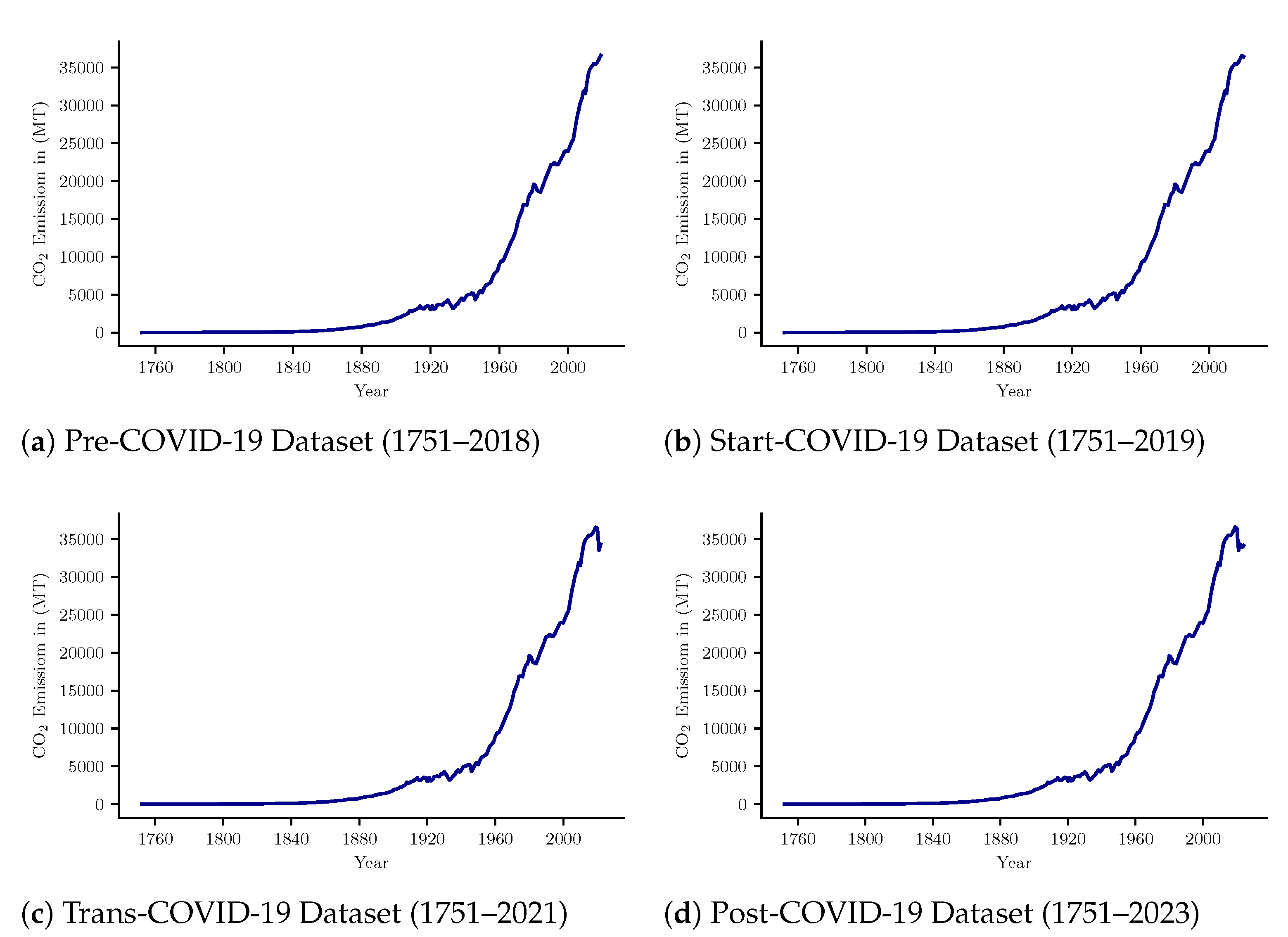
To augment data for the years from 2020 to 2023, the authors used the data from the source given here [1]. The respective changes in data for the other years were determined by considering the similar rates that were found in 2020 to 2021. The data trend is visualized in Figure 2. In Figure 1, actual and augmented data are clearly visible. Figure 2a,b present data from before the COVID-19 period. From Figure 2c, it can be seen that CO2 emissions decreased radically during the pandemic. Similar behavior can also be observed in Figure 2d for the remaining augmented cases such as 2021, 2022, etc. This data augmentation process takes advantage of developing the actual CO2 emission model to trace future emission behavior. Moreover, the data augmentation for near-term CO2 emissions will help to reduce modeling errors; thus, it helps in building real and suitable models. The best performing model can help in creating robust policies for the future to fight against CO2 emission problems across the world. For example, if one chooses to build a model based on the data available in Figure 2a, the model could predict wrong values. The model may not explain current or future emission behavior well during the changing environment of the pandemic. Moreover, there is a large chance that a forecasting model only based on data from 1751 to 2018 could be inaccurate. Seasonal data during COVID-19 should be included. The varied data values for different datasets are presented in Table 3.

2.4. Data Modeling

To model CO2 emissions, the authors used a time series-based ML technique named Autoregressive Integrated Moving Average (ARIMA) as well as Seasonal Autoregressive Integrated Moving Average (SARIMA). SARIMA is similar to ARIMA but seasonality is added to it. These two algorithms are regarded as the robust model and they are capable of presenting both stationary and non-stationary time series data. To forecast time series, three conditions need to be checked: (a) tentative identification, (b) parameter estimation and (c) diagnostic checking. Auto-regressive models are adroit in modeling different kinds of time series; (a) auto-regressive (AR), (b) moving average (MA), (c) auto-regressive moving average (ARMA) and (d) ARIMA. The base for the ARIMA model is the Box–Jenkin method [37]. ARIMA is written as ARIMA (p,d,q) where the seasonal parameter is absent and SARIMA is written as SARIMA (p, d, q) (P, D, Q) S where S is the seasonal parameter. During the ARIMA model optimization process S = 19 was found to be the best seasonality parameter, thus the ARIMA model turns into a SARIMA model and is presented as SARIMAX.
The SARIMA model can be written as:
φ p ( B ) Φ p ( B ) B S ( 1 B ) d ( 1 B S ) D Y t = θ q ( B ) Θ Q ( B S ) ε t
where:
φ p B = 1 φ 1 B φ 2 B 2 φ p B p
Φ p ( B ) B S = 1 Φ 1 B S Φ 2 B 2 S Φ p B p S
θ q ( B ) = 1 θ 1 B θ 2 B 2 θ q B q
Θ Q ( B S ) = 1 Θ 1 B S Θ 2 B 2 S Θ Q B Q S
In the equations above, t = 1 , 2 , 3 N ; N is the number of observations up to time t; B is the backshift operator defined by B α W t ; φ p ( B ) is called a regular (non-seasonal) autoregressive operator of order p; φ p ( B S ) is a seasonal autoregressive operator of order p; θ q ( B ) is a regular moving average operator of order q; Θ Q ( B S ) is a seasonal moving average operator of order Q; ε t is identically and independently distributed as normal random variables with mean zero, variance α 2 and c o v ( ε t ) , ε t k ) = 0 , k 0 ; p is the auto-regressive term; q is the moving average order; P is the seasonal period length of the model, S, of the auto-regressive term; Q represents the seasonal period length of the model, S, of the moving average order; D represents the order of seasonal differencing; d represents the order of ordinary differencing [38].
While fitting data to a SARIMA model, the values of d and D are estimated initially; this gives good results during seasonality issues. The remaining values of p, q and Q need to be chosen by the auto-correlation function (ACF) and the partial auto-correlation function (PACF). AFC and PACF were automatically calculated by the program developed for data modeling. To control overfilling in the models, hold-outs (test–train split), feature selection and data augmentation techniques were used.
To evaluate the model, we use some prediction metrics, namely mean absolute percentage error (MAPE) [39], mean squared error (MSE) [40], root mean squared error (RMSE) [39] and mean absolute deviation (MAD) [39]. For simplicity and integrity, MAPE scores were finally presented in this paper for model accuracy comparison.
To build different models, the ARIMA algorithm was repeatedly executed using the author-developed optimization algorithm. After checking efficiency issues, the most efficient model was used. Models that were found to be efficient with regard to this work were as follows; for the pre-COVID-19 period, the ARIMA (2,1,2)(0,1,1) [19] (SARIMAX(2, 1, 2)x(0, 1, 1, 19)) model with ACF = 0.88 and MAPE = 0.32; for the start-COVID-19 period, the ARIMA(1,1,2)(0,1,1) [19] (SARIMAX(1, 1, 2)x(0, 1, 1, 19)) model with ACF 0.93 and MAPE = 0.28; for the trans-COVID-19 period, the ARIMA(0,2,1)(1,1,1) [19] (SARIMAX(0, 2, 1)x(1, 1, 1, 19)) model with ACF 0.90 and MAPE = 0.19; and for the post-COVID-19 period, the ARIMA(0,2,1)(1,1,1) [19] (SARIMAX(0, 2, 1)x(1, 1, 1, 19)) model with ACF 0.88 and MAPE = 0.09.
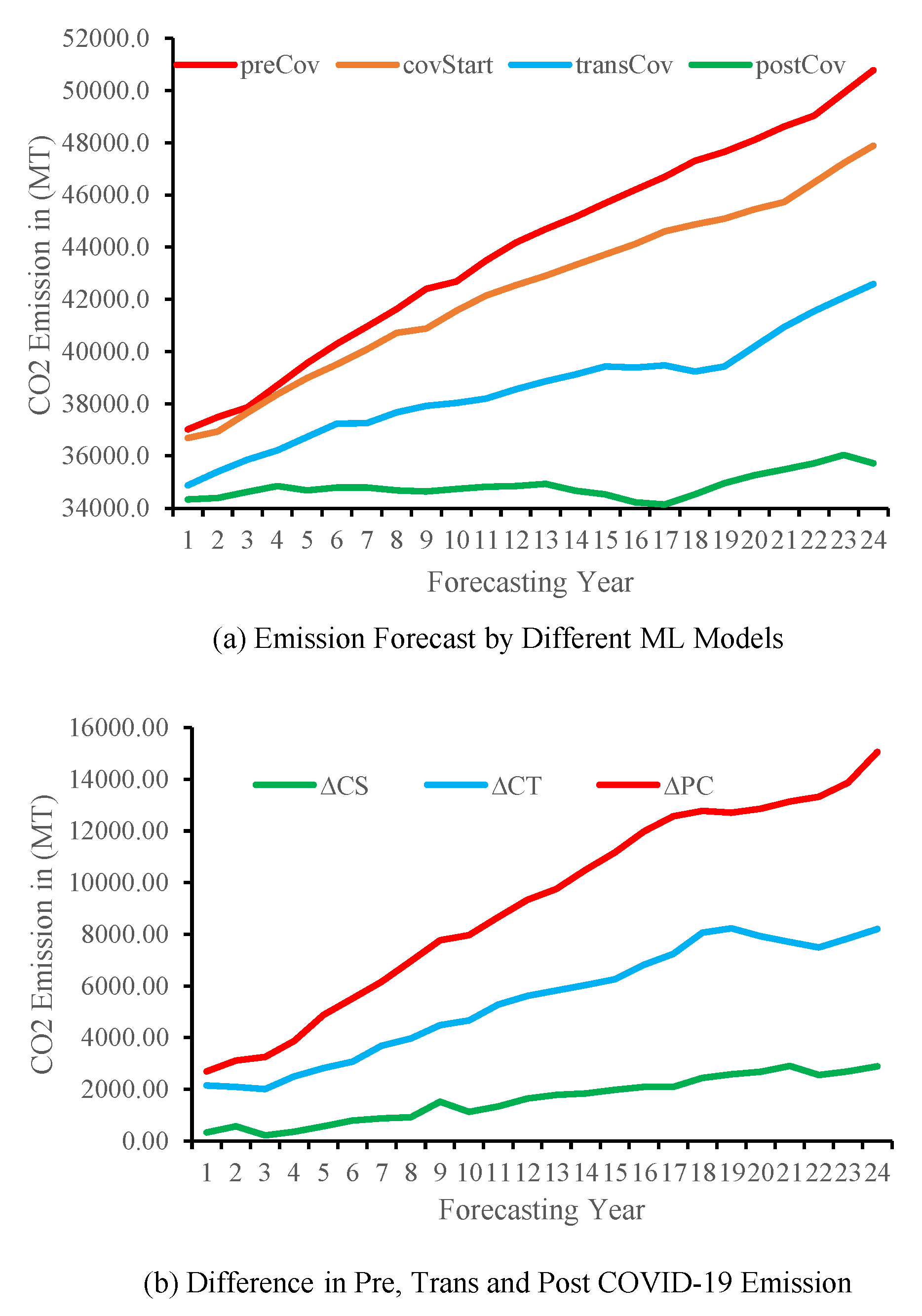
Here, the authors introduced three metrics, namely Δ C S , Δ C T and Δ P C , to calculate the forecasting value difference between different models to show the error propagation among different models. These metrics can show us the forecasting error between different models. This is the difference between the pre-COV (pre-COVID-19) model predicted values and the respective models during the COVID-19 surge (e.g., start-COVID-19, trans-COVID-19 and post-COVID-19). This means that if one chooses to forecast actual CO2 during and after the COVID-19 period, one needs to select any model other than pre-COVID-19; otherwise, a substantial error will spread in the forecasting value over time.
M A P E = t = 1 n | ( y t y t ^ ) / y t | n 100
M S E = t = 1 n ( y t y t ^ ) 2 n
R M S E = t = 1 n | y t y t ^ | n
M A D = t = 1 n | y t y t ^ | n
Δ C S = p r e C o v p r e d s t a r t C o v p r e d
Δ C T = p r e C o v p r e d t r a n s C o v p r e d
Δ P C = p r e C o v p r e d p o s t C o v p r e d
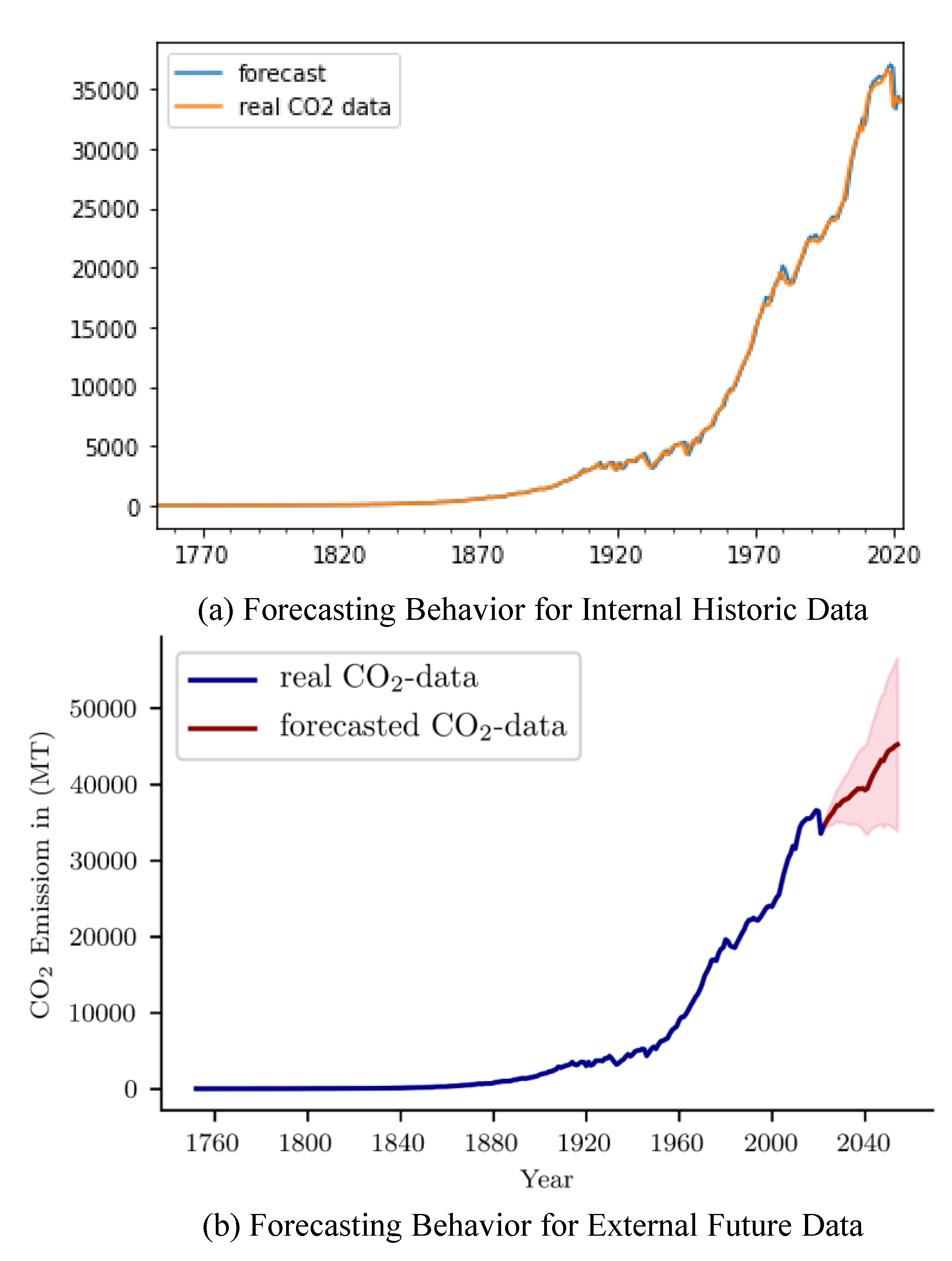
After the model is successfully developed, it is time to create visual representations of the modeling outcomes. Figure 3 and Figure 4 present the outcomes of the models that were built beforehand. Figure 3 presents the internal forecasting results related to the time period (either for 2018, 2019, 2020 or 2021) of the datasets and 
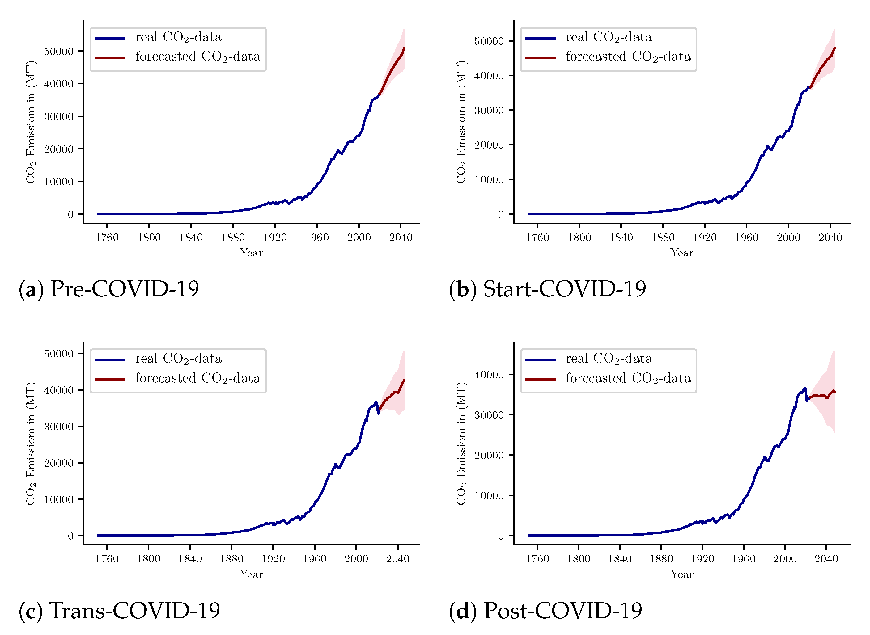
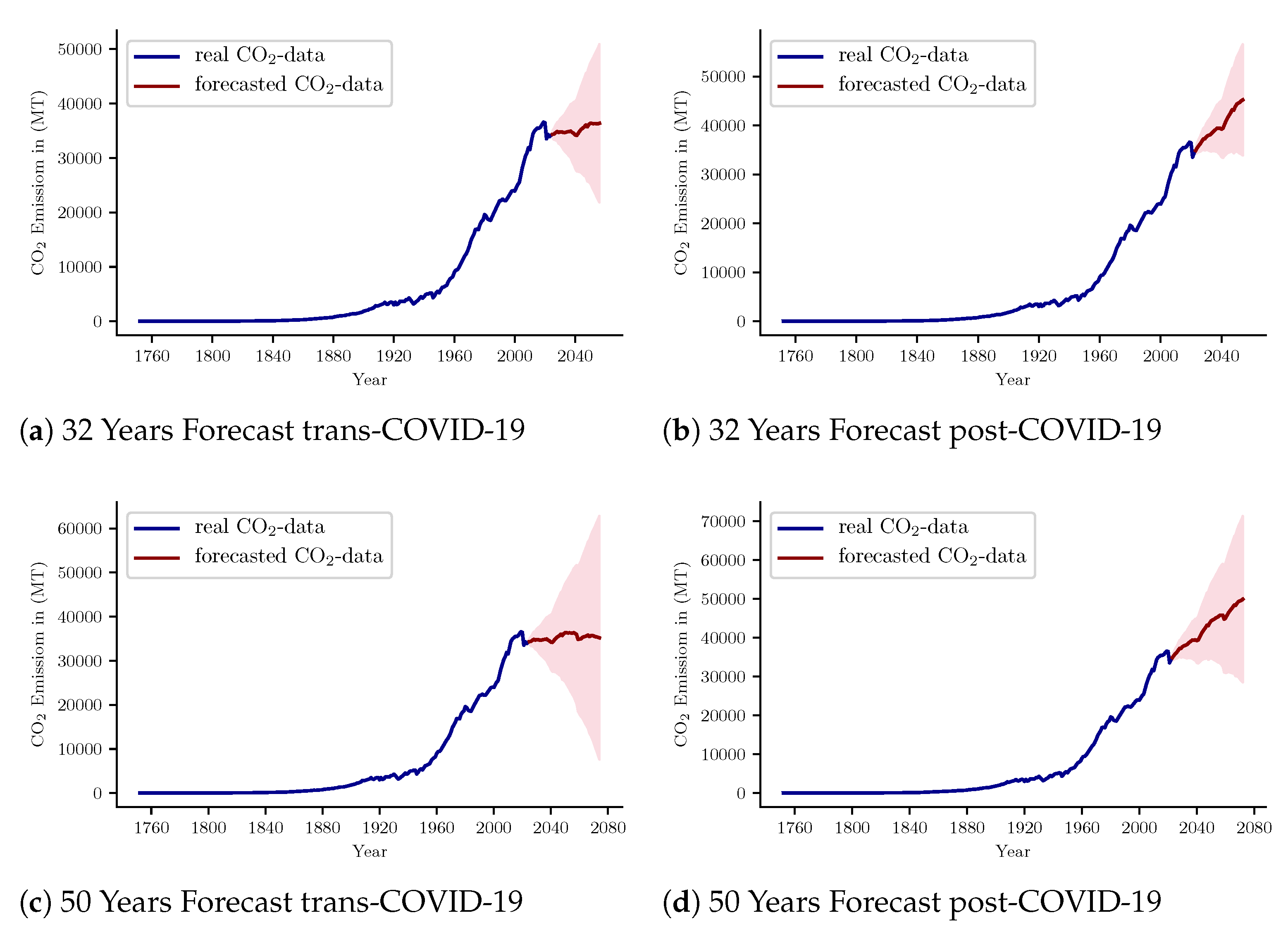
Figure 4 presents the external or future (time periods beyond the datasets, that is, 2022, 2023, etc.) forecasting behavior.
During data modeling, four things can happen—one can build a model: (1) based on the base data (pre-COVID-19 data as shown in Figure 2a) before the COVID-19 pandemic; (2) based on the data (start-COVID-19 data as shown in Figure 2b) when the COVID-19 pandemic starts surging; (3) based on the data (trans-COVID-19 data as shown in Figure 2c) while the COVID-19 pandemic is spreading globally; (4) based on the data (post-COVID-19 data as shown in Figure 2d) after the COVID-19 pandemic is over.
If one intended to build a CO2 emission model with option (1), forecasting results will probably not represent the real situation concerning emissions observed due to the COVID-19 pandemic. Option (2) would not be the justified option for the same reason, with regard to the period of the COVID-19 pandemic just beginning to spread over China. Option (3) would be the viable option for building a model to forecast CO2 emissions because in this time period the COVID-19 pandemic spreads over the world and massive lockdown processes have already shut down a huge number of CO2 emission sources acriss the world. Option (4) would be a supplementary one if COVID-19 finishes its surge over the globe in this period. The time span of 2022 to 2023 can be considered the period when the COVID-19 pandemic will finish its surge; if it is not, then this period can be considered as part of the extended transmission period. As seen from the global situation, the COVID-19 surge ended in 2021. So, option (4) can only be a post-COVID-19 situation.
If one wants to forecast the exact behavior of CO2 emissions well, these authors suggest building all four models (at least 3 models from 2 to 4), so that exact emission behavior can be covered. No single model can forecast the exact CO2 emissions well. These authors in the end chose a model the reflects the CO2 emissions in the near or far future.

2.5. Model Validation

To validate the models presented in this paper, Figure 3 is sufficient for the evidence. Figure 3 shows the forecasting behavior of emissions for the current (1751–2021) and future (2022 and beyond) years. The pink shadow in Figure 3 is the confidence interval (the upper and lower bound of forecast). Furthermore, a number of performance parameters are presented here to better understand the forecasting values. Table 4 presents the modeling error and accuracy parameters as found during the model development.
As seen from Table 5, the error scores for the models are 32%, 28%, 19% and 9% for the respective models. In accordance with Table 4 [41], the accuracy intensities for the respective models are named Reasonable, Reasonably Better, Accurate and Highly Accurate.
Hence, the best models are the models that use data from during the COVID-19 pandemic surge. The outcomes of the models exactly resemble the reality of CO2 emissions across the globe. As the COVID-19 pandemic reaches its mild stage across the globe and lockdowns end, this situation can be treated as the post-COVID-19 period. As a result, to be in line with the real world situation, the post-COVID-19 model actually reflects the current situation concerning CO
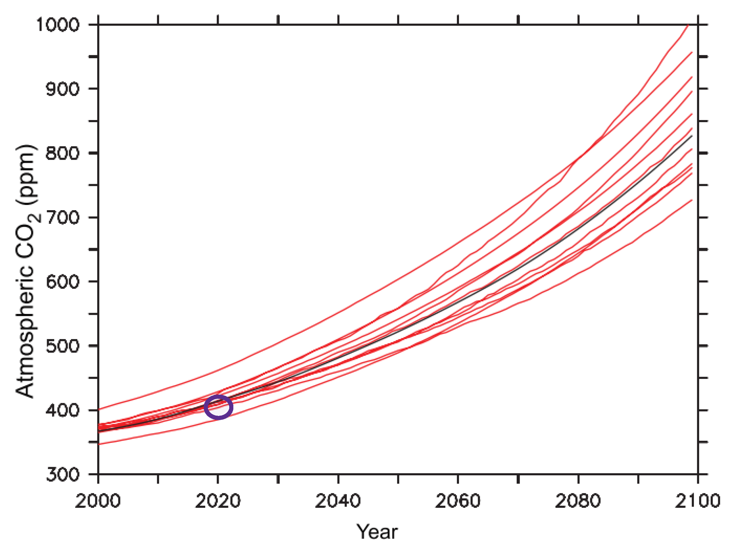
2 emissions. We predicted some values of CO2 emissions for a few years and compared them with real emission data [42] as well as a benchmark IPCC model [27]. The comparison results shows the model performs well against real world and benchmark IPCC models. All the results are measured in ppp and giga tons (GT). They are presented in Table 6.
As seen from Table 6, forecasting models are justified and accurate enough to represent real CO2 emission behavior for the current and near future. It is inferred that far future predictions would be justified too. For purposes of further forecasting, in the end the most accurate model (post-COVID-19 model) was chosen to present the different forecasting scenarios.

3. Results

A number of interesting and insightful results were found upon forecasting near–far future CO2 emissions using the accurate models. Near future results are used to validate the model. Afterwards, far future CO2 emissions are predicted. Results are presented in the following sections.

3.1. Near Future Emission Forecast

The selected Post-COVID-19 model was used to forecast the near future CO2 emission values. The model yields some empirical forecasting for the years selected. The forecasting results are shown in Table 7. These near future forecasting values will be the supportive evidence for the far future forecasting by the model.

3.2. Increasing Progression in CO2 Emission over Time

Forecast models show an increasing growth rate of CO2 emissions over time. This phenomenon can be seen for all the time periods. As seen from Figure 5b,d, the same progression rates were found for both the 32-year and the 50-year cases. The 24-year case involved a similar situation.This is consistent with earlier forecasts. As seen from Figure 5, in the case of historic data, the CO2 emission rate progressed after 1950 and this rate continued until the COVID-19 phenomenon observed in 2019. A similar upward progression will continue after the end of COVID-19 lockdowns. This progression rate might be lower only if the COVID-19 lockdown continues for a few more consecutive years. If that happens, then CO2 emissions could be similar as shown in Figure 5b,d.

3.3. Effects Similar to COVID-19 Can Heal the Environment

As seen from the previous discussion, the COVID-19 effect can slow down the increasing progression of CO2 emissions for a long time. In a low CO2 emission atmosphere, there is much greater scope for the environment to heal its wounds. The most suitable case of the healing process is shown in Figure 5a,c, where three years (2020–2023) assuming the COVID-19 effect (lockdown) slow down the high progression rate of emissions. If this (lockdown or similar) can occur a number of times in a year, the progression rate can be lowered even more. A similar effect can be artificially induced by every nation so that CO2 emissions decrease to a minimal level. Recently, Japan has been thinking of reducing its working days to 4 days a week. Microsoft Japan already implemented this program experimentally and found success [44].

3.4. Consecutive CO2 Emission Reduction Can Reduce Overall Emission Trend

Due to consecutive lockdowns across the world, a number of CO2 emission sources have stopped emitting. As a result, the CO2 footprint is lower than before. This phenomenon can be seen in Figure 5a,c. Here, only three years (2021, 2022, 2023) with reduced CO2 emissions were involved. This little change in emissions has changed the overall emission pattern for a long time. With this result, a policy can be created to introduce artificial lockdown-like situations across nations to reduce CO2 emissions to a viable point.

3.5. COVID-19 Helps Noticeable CO2 Emission Reduction

As we have, COVID-19 has decreased CO2 emissions to a significant extent. Here, we quantify the reduction footprint. As seen from Figure 6a, CO2 emissions for the post-COVID-19 case (2022, 2023) are less than 3000 MT to 15,000 MT depending on the years addressed in the forecasting. A similar event can be observed for the transition course (2020, 2021) of COVID-19 (shown in blue). This different forecasting behavior is significant with regard to making a decision concerning developing policies with respect to which model to use for what kind of emission.

3.6. Long Lockdown Means Less CO2 Emission

An assumed lockdown for the case of the years 2020 to 2023 changed the forecasting value dramatically. These reduced values have many rational effects on the earth—the home of thousands of species. From Figure 6b, it is clearly visible that Δ P C is far bigger than Δ C S and Δ C T is in between the two. Here, Δ P C , Δ C S and Δ C T are the forecasting value differences between post-COVID-19, start-COVID-19 and trans-COVID-19, respectively. As seen from Δ P C in Figure 6b, 3000 MT to 15,000 MT CO2 less than the normal case Δ C S is emitted. This lesser emission of CO2 can save a lot of resources across the world. This reduced CO2 emission could be helpful concerning greenhouse effects, glacier ice melting, unexpected climate change, desertification, saltification of fresh water and soils near coastal areas and many more things which are harmful to the environment for the planet earth.

4. Discussion

All previous research presented in the literature had projected and modeled CO2 emissions using data collected prior to the COVID-19 pandemic. Without accounting for the effects of COVID-19 on CO2 emissions, predictions might include inaccuracies. This study accounted for COVID-19’s effect on CO2 emissions by including data from the previous declining trend. This yields realistic CO2 emission predictions (up to 2000 MT reduction). Failing to account for COVID-19’s effect on CO2 emissions might make the prediction result more unrealistic (prediction difference is up to 15,000 MT). Mild prediction accuracy can also be observed for the COVID-19 transition period (prediction values up to 7000 MT). All the scenarios can be seen in Figure 6b. Hence, accounting for COVID-19’s effect on CO2 emissions yields realistic future CO2 emission values.
On the other hand, the method used in this paper maps the predicted CO2 emission values accurately. The maximum accuracy of model was 91%. Thus, the models developed are less error prone. Hence, the model-predicted CO2 emission data and the accuracy data converged. As a result, the method and predicted CO2 emissions can be considered accurate and worth using. This claim is verified in Table 8.
This paper is successful in terms of developing a robust and accurate CO2 emission prediction model accounting for COVID-19-driven lockdown effects. It also delivered a number of meaningful and interesting insights from the historic data. The model is more accurate concerning CO2 emission prediction than previous models. The model can be used to predict CO2 emissions, to create policies for CO2 emission reduction, and for CO2 emission tracing. This modeling approach and the solution yielded can be considered new additions to the respective domains of knowledge.
In this paper, the authors focused on developing an optimized CO2 emission prediction model. The work can be further extended by developing complete web or mobile applications to trace CO2 emissions with the touch of finger tip. A comprehensive digital twin could also be developed for CO2 emissions. All such works are options for future.

5. Conclusions

Carbon emissions, the greenhouse effect, climate change and catastrophic environmental issues have become the most crucial issues in the contemporary world. Application of AI and ML have a significant impact in terms of solving these issues. This work focuses on using AI to develop an ML model for global total CO2 emissions to forecast CO2 emissions for the near or far future. Building ML models considering reduced CO2 emissions during the COVID-19 pandemic, we found some noticeable outcomes which can help in understanding CO2 emissions across the world. The MAPEs for the four methods are: pre-COV (MAPE: 0.32), start-COV (MAPE: 0.28), trans-COV (MAPE: 0.19), post-COV (MAPE: 0.09), where the selected model to predict future CO2 emission behavior has a MAPE of 9%. This is quite good accuracy with respect to the data available at hand. The post-COV model predicted global total CO2 emissions for the years 2022 to 2027 are: 36,218.59, 36,733.69, 37,238.29, 37,260.88, 37,674.01 and 37,921.47 MT. By comparing our forecasting output to current and previous benchmark work, one can validate the obtained accuracy. Consequently, the forecasting of CO2 emissions for the far future years should be accurate.
In this work, the post-COVID-19 model forecasts reasonable CO2 emission behavior. Moreover, the trans-COVID-19 model shows some remarkable forecasts. Whatever the forecast we obtained, it may not actually reflect the real CO2 emission practically. Moreover, a number of external influencing features need to be considered in future developments. Moreover, some other optimization methods or feature selections could be applied. All the remaining issues could be further explored in future research.
Further observations of this study are given below:
  • The AI-based ML method can help to forecast CO2 emission behavior during or after the COVID-19 pandemic.
  • Lockdown-like situations can reduce CO2 emissions in the present and in the far future.
  • Artificial lockdowns or shorter (e.g., 4 days) working schedules can help to heal the environment.
  • A policy can be created to impose artificial lockdown-like events to reduce the overall CO2 emission footprint.

Author Contributions

Conceptualization, Y.M. and; methodology, Y.M.; software, Y.M.; validation, H.N.; formal analysis, Y.M.; investigation, Y.M.; resources, Y.M.; data curation, Y.M.; writing—original draft preparation, Y.M.; writing—review and editing, H.N.; visualization, Y.M.; supervision, Y.M.; project administration, Y.M.; funding acquisition, Y.M. All authors have read and agreed to the published version of the manuscript.

Funding

This research received no external funding.

Institutional Review Board Statement

Not applicable.

Informed Consent Statement

Not applicable.

Data Availability Statement

Data used in this article is cited in the reference section. More curated data is also available by a request to the corresponding author.

Acknowledgments

This work is owed to the assistant of Noman Hossain and his team for their cooperation and data acquisition role. It is worth mentioning some names those who are not written herein. This work is also grateful to the respective institutions for their instrumental support.

Conflicts of Interest

The authors declare no conflict of interest.

References

  1. Global Energy Review 2020. Available online: https://www.iea.org/reports/global-energy-review-co2-emissions-in-2021-2 (accessed on 16 October 2022).
  2. Singh, P.K.; Pandey, A.K.; Ahuja, S. Multiple forecasting approach: A prediction of CO2 emission from the paddy crop in India. Environ. Sci. Pollut. Res. Vol. 2022, 29, 25461–25472. [Google Scholar] [CrossRef] [PubMed]
  3. Ağbulut, Ü. Forecasting of transportation-related energy demand and CO2 emissions in Turkey with different machine learning algorithms. Sustain. Prod. Consum. 2022, 29, 141–157. [Google Scholar] [CrossRef]
  4. Demir, A.S. Modeling and forecasting of CO2 emissions resulting from air transport with genetic algorithms: The United Kingdom case. Theor. Appl. Climatol. 2022, 150, 777–785. [Google Scholar] [CrossRef] [PubMed]
  5. Wang, H.; Zhang, Z. Forecasting CO2 Emissions Using a Novel Grey Bernoulli Model: A Case of Shaanxi Province in China. Int. J. Environ. Res. Public Health 2018, 19, 1–22. [Google Scholar]
  6. Ahn, K.U.; Kim, D.W.; Cho, K.; Cho, D.; Cho, H.M.; Chae, C.U. Hybrid Model for Forecasting Indoor CO2 Concentration. Buildings 2022, 12, 1540. [Google Scholar] [CrossRef]
  7. Iania, L.; Algieri, B.; Leccadito, A. Forecasting Total Energy’s CO2 Emissions, LIDAM Discussion Paper LFIN. 2022, pp. 1–58. Available online: https://ssrn.com/abstract=4116768 (accessed on 10 October 2022).
  8. Zhong, W.; Haigh, J.D. The greenhouse effect and carbon dioxide. Weather 2013, 68, 100–105. [Google Scholar] [CrossRef]
  9. Cook, J.; Oreskes, N.; Doran, P.T.; Anderegg, W.R.; Verheggen, B.; Maibach, E.W.; Rice, K. Consensus on consensus: A synthesis of consensus estimates on human-caused global warming. Environ. Res. Lett. 2016, 11, 048002. [Google Scholar] [CrossRef]
  10. Myers, K.F.; Doran, P.T.; Cook, J.; Kotcher, J.E.; Myers, T.A. Consensus revisited: Quantifying scientific agreement on climate change and climate expertise among Earth scientists 10 years later. Environ. Res. Lett. 2016, 16, 104030. [Google Scholar] [CrossRef]
  11. Florides, G.A.; Christodoulides, P. Global warming and carbon dioxide through sciences. Environ. Int. 2009, 35, 390–401. [Google Scholar] [CrossRef]
  12. Solomon, S.; Plattner, G.K.; Knutti, R.; Friedlingstein, P. Irreversible climate change due to carbon dioxide emissions. Proc. Natl. Acad. Sci. USA 2009, 106, 1704–1709. [Google Scholar] [CrossRef] [Green Version]
  13. Lane, J. CO2 emissions and GDP. Int. J. Soc. Econ. 2011, 38, 911–918. [Google Scholar] [CrossRef]
  14. Chang, C.L.; Ilomäki, J.; Laurila, H.; McAleer, M. Causality between CO2 emissions and stock markets. Energies 2020, 13, 2893. [Google Scholar] [CrossRef]
  15. Sharma, S.; Zhang, M.; Gao, J.; Zhang, H.; Kota, S.H. Effect of restricted emissions during COVID-19 on air quality in India. Sci. Total. Environ. 2020, 728, 138878. [Google Scholar] [CrossRef] [PubMed]
  16. Franceschi, F.; Cobo, M.; Figueredo, M. Discovering relationships and forecasting PM10 and PM2.5 concentrations in Bogotá Colombia, using Artificial Neural Networks, Principal Component Analysis and k-means clustering. Atmos. Pollut. Res. 2018, 9, 912–922. [Google Scholar] [CrossRef]
  17. Qian, Y.; Sun, L.; Qiu, Q.; Tang, L.; Shang, X.; Lu, C. Analysis of CO2 drivers and emissions forecast in a typical industry-oriented county: Changxing County, China. Energies 2020, 13, 1212. [Google Scholar] [CrossRef] [Green Version]
  18. Zhou, J.; Yu, X.; Guang, F.; Li, W. Analyzing and predicting CO2 emissions in China based on the LMDI and GA-SVM model. Pol. J. Environ. Stud. 2018, 27, 927–938. [Google Scholar] [CrossRef]
  19. Sun, W.; Sun, J. Prediction of carbon dioxide emissions based on principal component analysis with regularized extreme learning machine: The case of China. Environ. Eng. Res. 2017, 22, 302–311. [Google Scholar] [CrossRef] [Green Version]
  20. Safa, M.; Nejat, M.; Nuthall, P.L.; Greig, B.J. Predicting CO2 Emissions from Farm Inputs in Wheat Production using Artificial Neural Networks and Linear Regression Models. Int. J. Adv. Comput. Sci. Appl. 2016, 7, 268–274. [Google Scholar] [CrossRef] [Green Version]
  21. Shabani, E.; Hayati, B.; Pishbahar, E.; Ghorbani, M.A.; Ghahremanzadeh, M. A novel approach to predict CO2 emission in the agriculture sector of Iran based on Inclusive Multiple Model. J. Clean. Prod. 2021, 279, 123708. [Google Scholar] [CrossRef]
  22. Ahmadi, M.H.; Jashnani, H.; Chau, K.W.; Kumar, R.; Rosen, M.A. Carbon dioxide emissions prediction of five Middle Eastern countries using artificial neural networks. Energy Sources Part Recover. Util. Environ. Eff. 2019, 1–13. [Google Scholar] [CrossRef]
  23. Liu, Z.; Ciais, P.; Deng, Z.; Davis, S.J.; Zheng, B.; Wang, Y.; Cui, D.; Zhu, B.; Dou, X.; Ke, P.; et al. Carbon Monitor, a near-real-time daily dataset of global CO 2 emission from fossil fuel and cement production. Sci. Data 2020, 7, 2052–4463. [Google Scholar] [CrossRef] [PubMed]
  24. Tanania, V.; Shukla, S.; Singh, S. Time series data analysis and prediction of CO2 emissions. In Proceedings of the Confluence 2020 10th International Conference on Cloud Computing, Data Science and Engineering, Noida, India, 29–31 January 2020; pp. 665–669. [Google Scholar]
  25. Dong, F.; Yu, B.; Pan, Y. Examining the synergistic effect of CO 2 emissions on PM 2.5 emissions reduction: Evidence from China. J. Clean. Prod. 2019, 223, 759–771. [Google Scholar] [CrossRef]
  26. Rolnick, D.; Donti, P.L.; Kaack, L.H.; Kochanski, K.; Lacoste, A.; Sankaran, K.; Ross, A.S.; Milojevic-Dupont, N.; Jaques, N.; Waldman-Brown, A.; et al. Tackling Climate Change with Machine Learning. ACM Computing Surveys 2022, 55, 1–96. [Google Scholar] [CrossRef]
  27. Meehl, G.A.; Stocker, T.F.; Collins, W.D.; Friedlingstein, P.; Gaye, A.T.; Gregory, J.M.; Kitoh, A.; Knutti, R.; Murphy, J.M.; Noda, A.; et al. Global Climate Projections. In Climate Change 2007: The Physical Science Basis. Contribution of Working Group I to the Fourth Assessment Report of the Intergovernmental Panel on Climate Change; Solomon, S., Qin, D., Manning, M., Averyt, K., Marquis, M., Eds.; Cambridge University Press: Cambridge, UK, 2007; Chapter 10; p. 790. [Google Scholar]
  28. Kadam, P.; Vijayumar, S. Prediction Model: CO2 Emission Using Machine Learning. In Proceedings of the 3rd International Conference for Convergence in Technology, I2CT 2018, Pune, India, 6–8 April 2018; pp. 1–3. [Google Scholar]
  29. Li, M.; Wang, W.; De, G.; Ji, X.; Tan, Z. Forecasting carbon emissions related to energy consumption in Beijing-Tianjin-Hebei region based on grey prediction theory and extreme learning machine optimized by support vector machine algorithm. Energies 2018, 11, 2475. [Google Scholar] [CrossRef] [Green Version]
  30. Kunda, D.; Phiri, H. An Approach for Predicting CO2 Emissions using Data Mining Techniques. Int. J. Comput. Appl. 2017, 172, 7–10. [Google Scholar] [CrossRef]
  31. Libao, Y.; Tingting, Y.; Jielian, Z.; Guicai, L.; Yanfen, L.; Xiaoqian, M. Prediction of CO2 Emissions Based on Multiple Linear Regression Analysis. Energy Procedia 2017, 105, 4222–4228. [Google Scholar] [CrossRef]
  32. Saleh, C.; Dzakiyullah, N.R.; Nugroho, J.B. Carbon dioxide emission prediction using support vector machine. IOP Conf. Ser. Mater. Sci. Eng. 2016, 114, 012148. [Google Scholar] [CrossRef]
  33. Deniz, S.; Gökçen, H.; Nakhaeizadeh, G. Application of Data Mining Methods for Analyzing of the Fuel Consumption and Emission Levels. Int. J. Eng. Sci. Technol. 2016, 5, 377–389. [Google Scholar]
  34. Saleh, C.; Chairdino Leuveano, R.A.; Ab Rahman, M.N.; Md Deros, B.; Dzakiyullah, N.R. Prediction of CO2 emissions using an artificial neural network: The case of the sugar industry. Adv. Sci. Lett. 2015, 21, 3079–3083. [Google Scholar] [CrossRef]
  35. Chen, Y.; Li, B.; Li, Z.; Shi, X. Quantitatively evaluating the effects of CO2 emission on temperature rise. Quat. Int. 2014, 336, 171–175. [Google Scholar] [CrossRef]
  36. Ritchie, H.; Roser, M.; Rosado, P. CO2 and Greenhouse Gas Emissions. Our World in Data. 2020. Available online: https://ourworldindata.org/co2-and-other-greenhouse-gas-emissions (accessed on 9 October 2022).
  37. Box, G. A Very British Affair Box and Jenkins: Time series analysis, forecasting and control. In A Very British Affair; Palgrave Macmillan: London, UK, 2016; pp. 161–215. [Google Scholar]
  38. Bai, L.; Wang, J.; Ma, X.; Lu, H. Air pollution forecasts: An overview. Int. J. Environ. Res. Public Health 2018, 15, 780. [Google Scholar] [CrossRef] [PubMed]
  39. IPM Insights Metrics. Available online: https://docs.oracle.com/en/cloud/saas/planning-budgeting-cloud/pfusu/insights_metrics.html (accessed on 10 October 2022).
  40. Sammut, C.; Webb, G.I. (Eds.) Mean Squared Error. In Encyclopedia of Machine Learning; Springer: Boston, MA, USA, 2021; Available online: https://doi.org/10.1007/978-0-387-30164-8_528 (accessed on 10 October 2022).
  41. Lewis, C.D. Industrial and business forecasting methods. Econ. J. 1982, 38, 414–425. [Google Scholar]
  42. Annual Global CO2 Emissions. Available online: https://www.co2.earth/global-co2-emissions (accessed on 12 October 2022).
  43. Atmospheric CO2 Levels (PPM). Available online: https://www.co2.earth/annual-co2 (accessed on 12 October 2022).
  44. Microsoft Japan Tested a Four-Day Work Week and Productivity Jumped by 40%. Available online: https://www.theguardian.com/technology/2019/nov/04/microsoft-japan-four-day-work-week-productivity (accessed on 6 July 2021).
Figure 1. CO2 Emission Forecasts by IPCC Model [27].
Atmosphere 13 01871 g001
Figure 2. CO2 Emission Dataset Visualization.
Atmosphere 13 01871 g002
Figure 3. CO2 Emission Forecasting Behavior for Internal and External Time.
Atmosphere 13 01871 g003
Figure 4. CO2 Emission Forecasting Behavior for Different Cases of Data.
Atmosphere 13 01871 g004
Figure 5. CO2 Emission Near–Far Forecasting Behavior for 32 and 50 Years.
Atmosphere 13 01871 g005
Figure 6. CO2 Emission Forecast Value Difference for Different ML Models.
Atmosphere 13 01871 g006
Table 1. Summery of Literature Review on CO2 Emission Forecast.
Article  Method  Accuracy  Context  Findings  
[28]ML(Regression)RMSE 25.57%GlobalAchieve low RMSE
[29]SVM-ELMRMSE 12.34%ChinaCO2 prediction up to 2030
[19]PCARMSE 0.3%ChinaCO2 prediction up to 2014
[30]WEKA-ZambiaForecast CO2 emission
[31]RegressionError 2.5%ChinaAccuracy in prediction
[20]ANNMSE 11%New ZealandBetter accuracy
[32]SVMMSE 0.04%IndonesiaEffective decision making
[33]Data Mining-Vehicular dataAccuracy in prediction
[34]ANNRMSE 5.5%Sugar IndustryAccuracy in prediction
[35]Quantitative-Global50.2% increase of temperature
[27]C 4 MIP modelMSE (10–20)%GlobalAccuracy in prediction
Table 2. CO2 Emission Datasets.
Dataset NameTime Period
pre-COVID-191751–2018
start-COVID-191751–2019
trans-COVID-191751–2021
post-COVID-191751–2023
Table 3. Augmented Values of CO2 Emissions in Various Datasets.
Dataset NameYearValues
pre-COVID-19201836,572.75
start-COVID-19201936,441.45
trans-COVID-19202034,226.18
trans-COVID-19202136,190.82
post-COVID-19202233,900.52
post-COVID-19202334,164.68
Table 4. Performance Parameters for CO2 Emission Models.
DatasetModelMAPEAccuracy
pre-COVID-19ARIMA(2,1,2)(0,1,1) [19]0.32Reasonable
start-COVID-19ARIMA(1,1,2)(0,1,1) [19]0.28Reasonably Better
trans-COVID-19ARIMA(0,2,1)(1,1,1) [19]0.19Accurate
post-COVID-19ARIMA(0,2,1)(1,1,1) [19]0.09Highly Accurate
Table 5. Interpretation of Typical MAPE Value.
MAPEInterpretation
>50%Inaccurate Forecasting
20–50%Reasonably Forecasting
10–20%Accurate Forecasting
10%Highly Accurate Forecasting
Table 6. Validation of CO2 Emission Forecast measured in (ppm-GT).
YearCurrent [42]IPCC [27]Our ModelAuthorś Remarks
2022415.76 [43]–Yet to get405–36.07409–36.45Accurate Forecast
2021413.79 [43]–36.4402–35.83406–36.18Highly Accurate Forecast
2020412.44 [43]–34.8400–35.65395–35.20Accurate Forecast
2019410.07 [43]–36.7398–35.57408.85–36.44Accurate Forecast
Table 7. Near Future CO2 Emission Forecast (MT).
YearCO2 Emission
202236,218.59
202336,733.69
202437,238.29
202537,260.88
202637,674.01
202737,921.47
Table 8. CO2 Emissions (GT), Current vs. Forecast.
YearCurrentOur Model
202236.45
202136.436.18
202034.835.20
201936.736.44
Publisher’s Note: MDPI stays neutral with regard to jurisdictional claims in published maps and institutional affiliations.

