
Spatially Resolved Source Apportionment of Industrial VOCs Using a Mobile Monitoring Platform

Abstract
:1. Introduction
2. Materials and Methods
2.1. Monitoring Area
2.2. Mobile Monitoring Platform
2.3. PTR-ToF-MS Measurements
2.4. PTR-ToF-MS Data Processing and PMF Analysis
3. Results
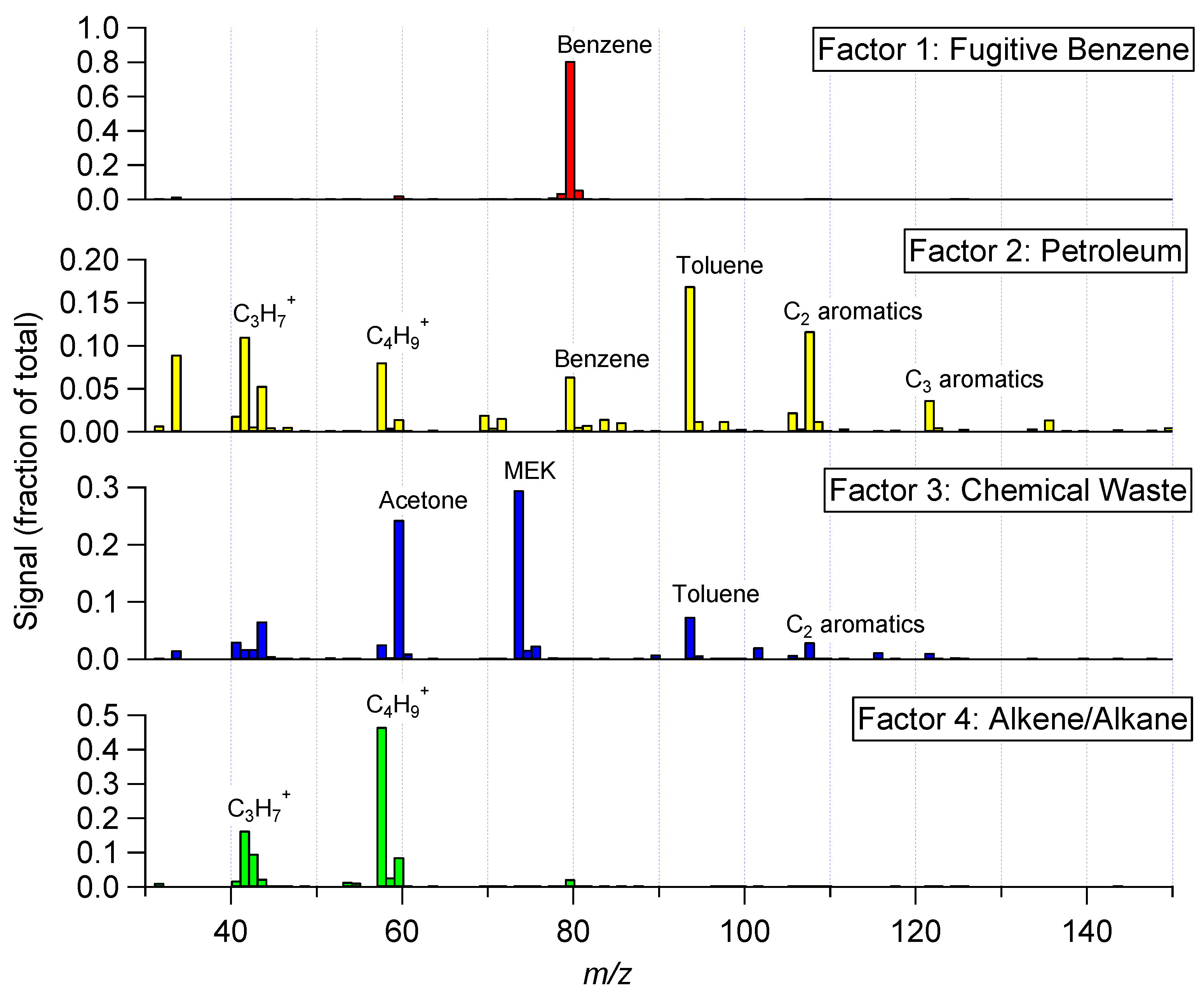
3.1. PMF Results
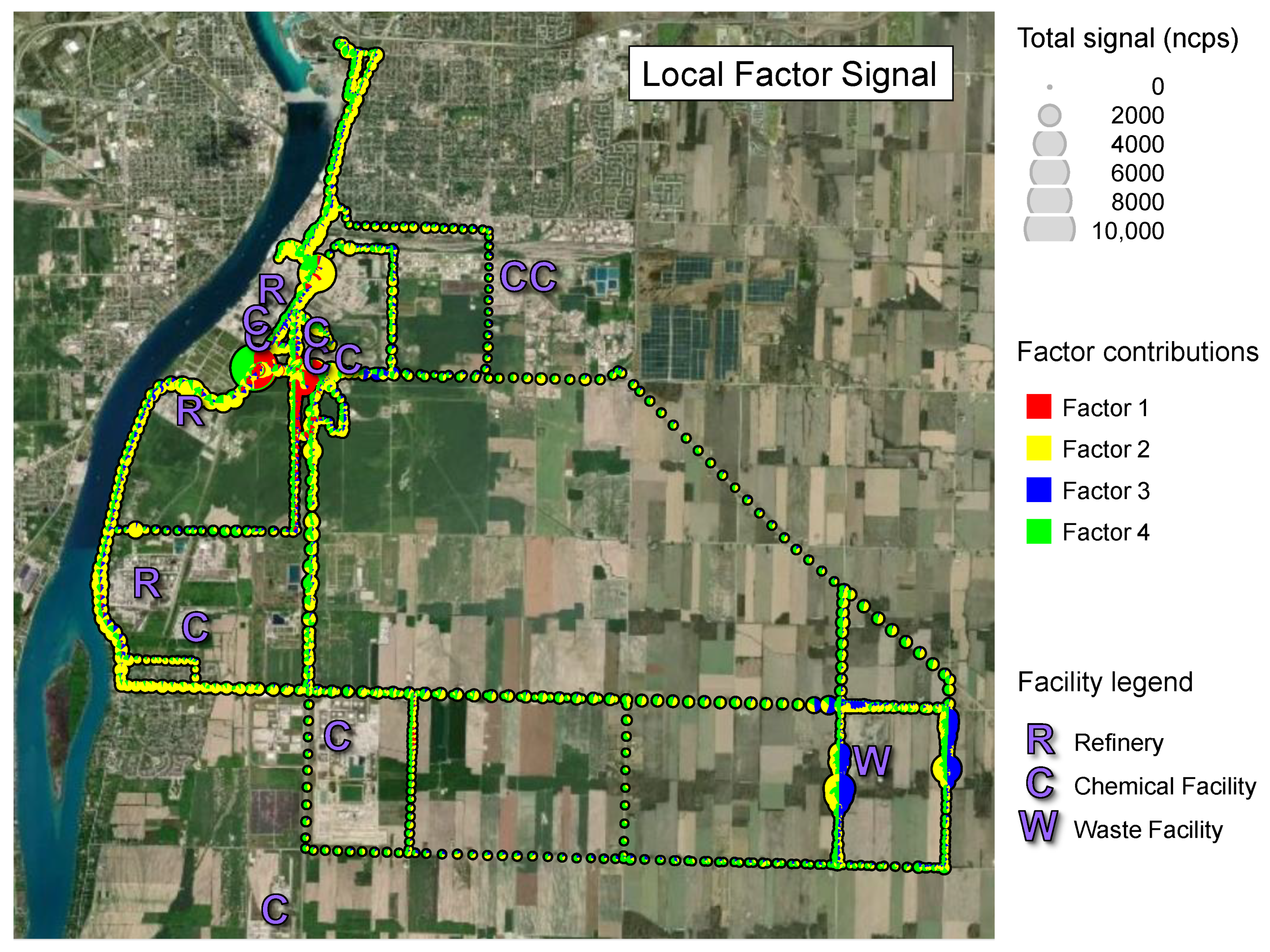
3.2. Spatially Resolved Apportionment: Local Factor Contributions
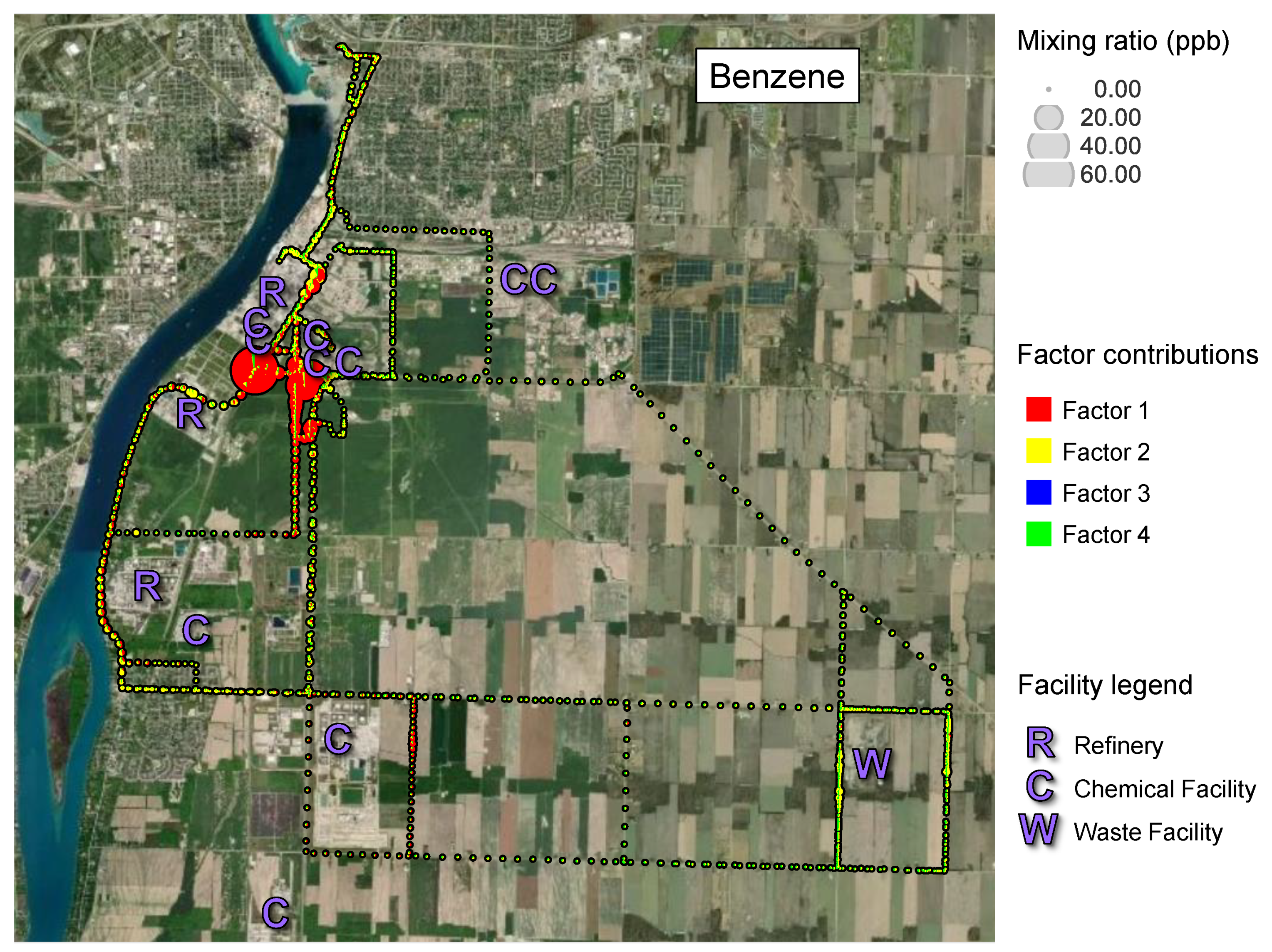
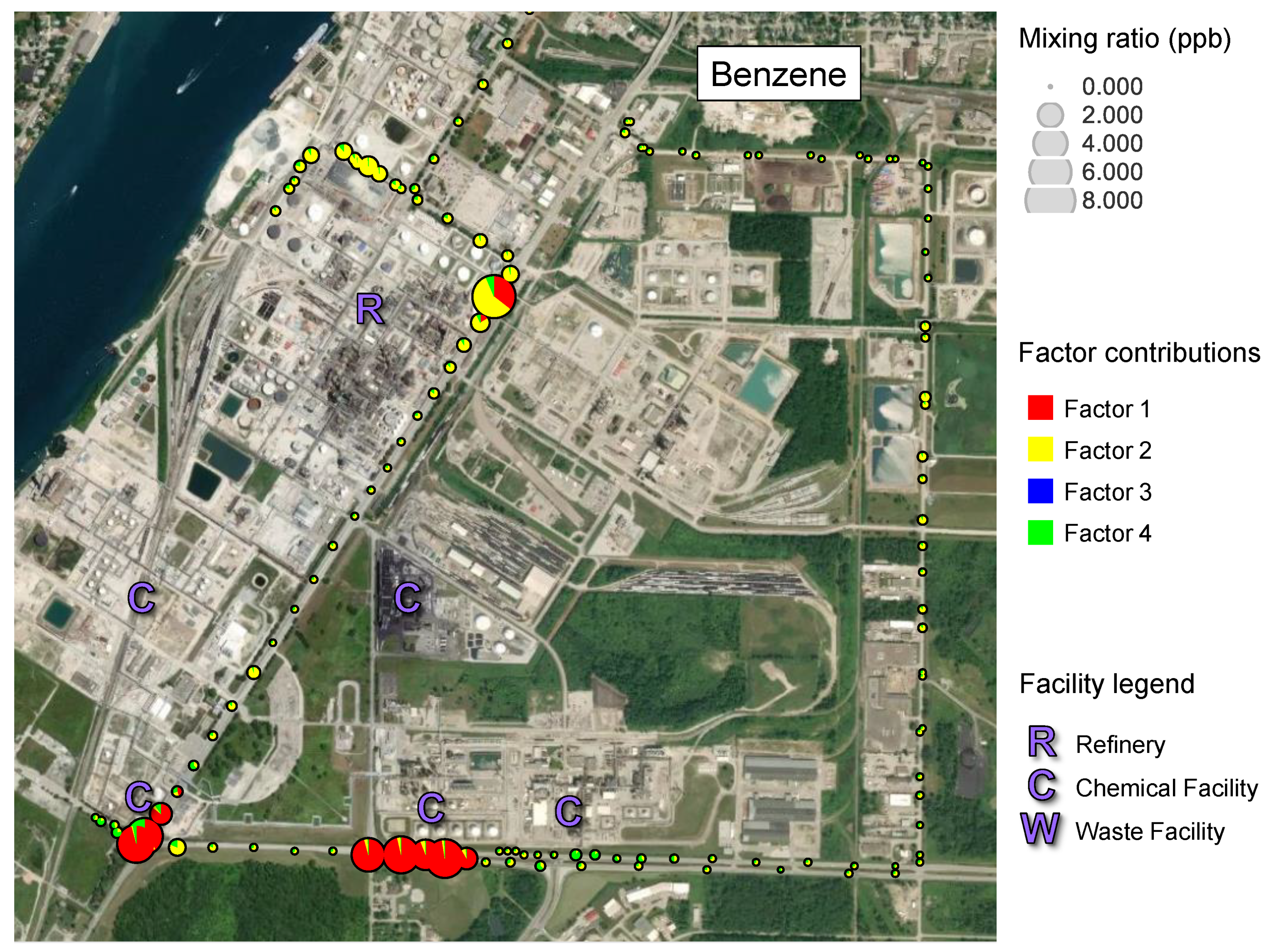
3.3. Spatially Resolved Apportionment: Benzene
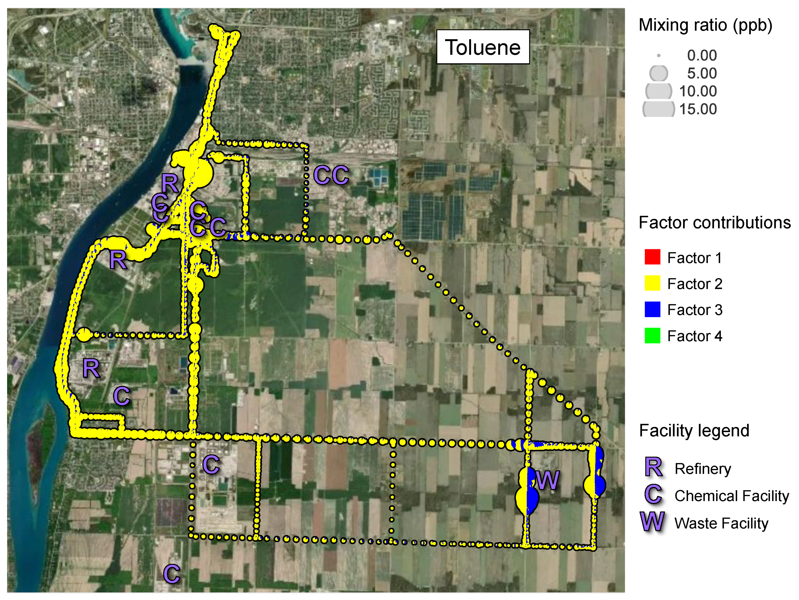
3.4. Spatially Resolved Apportionment: Toluene
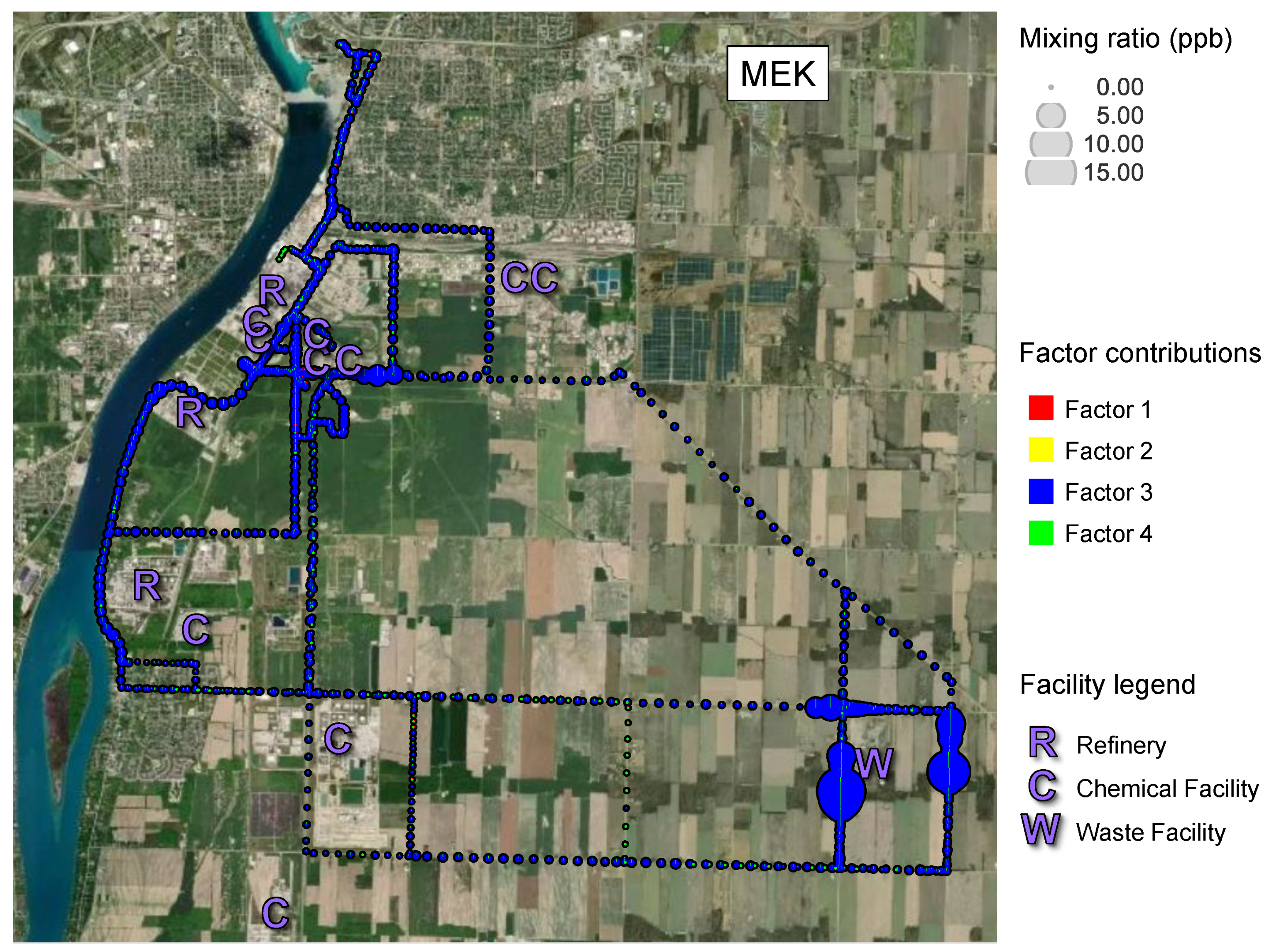
3.5. Spatially Resolved Apportionment: MEK
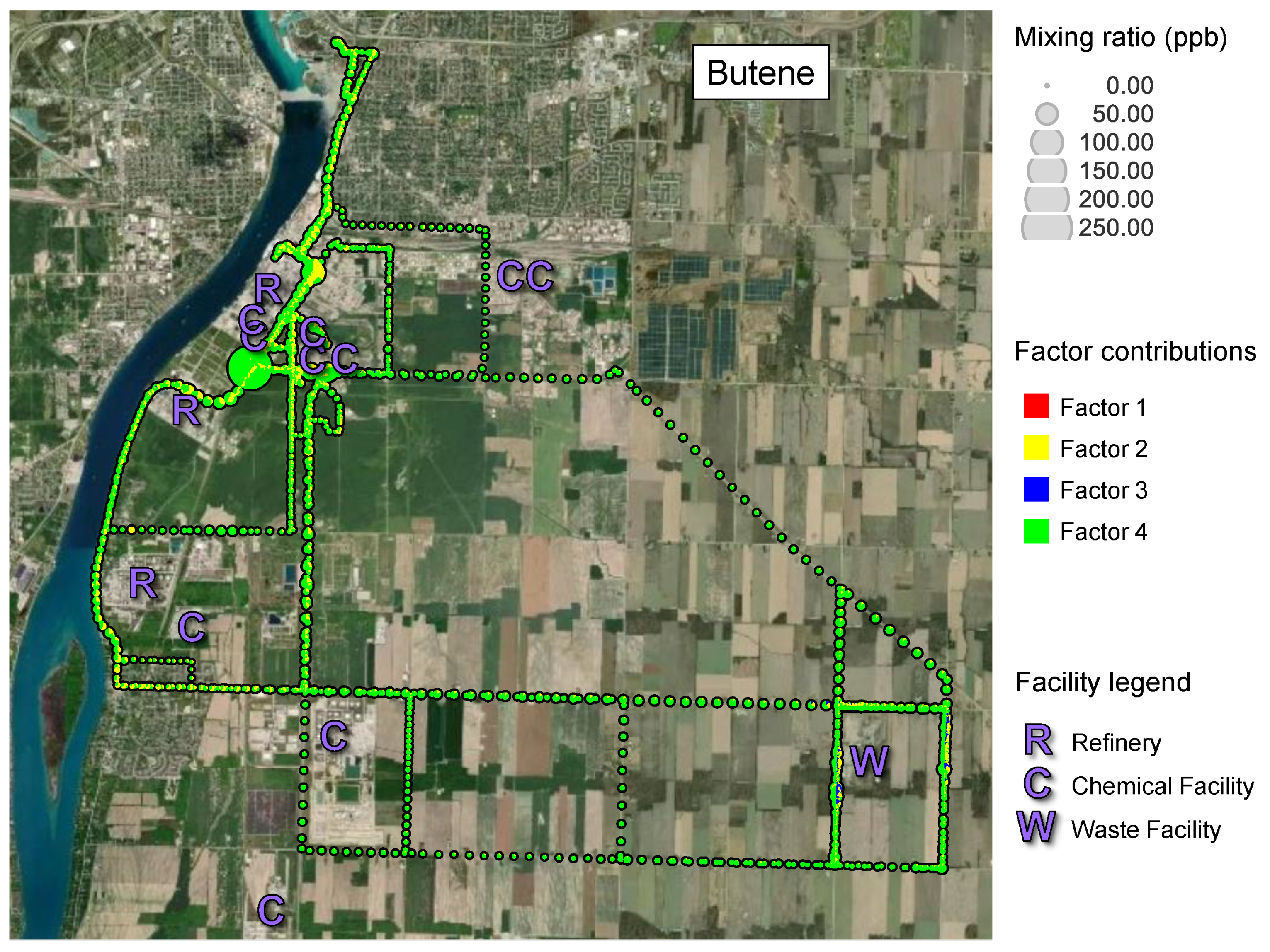
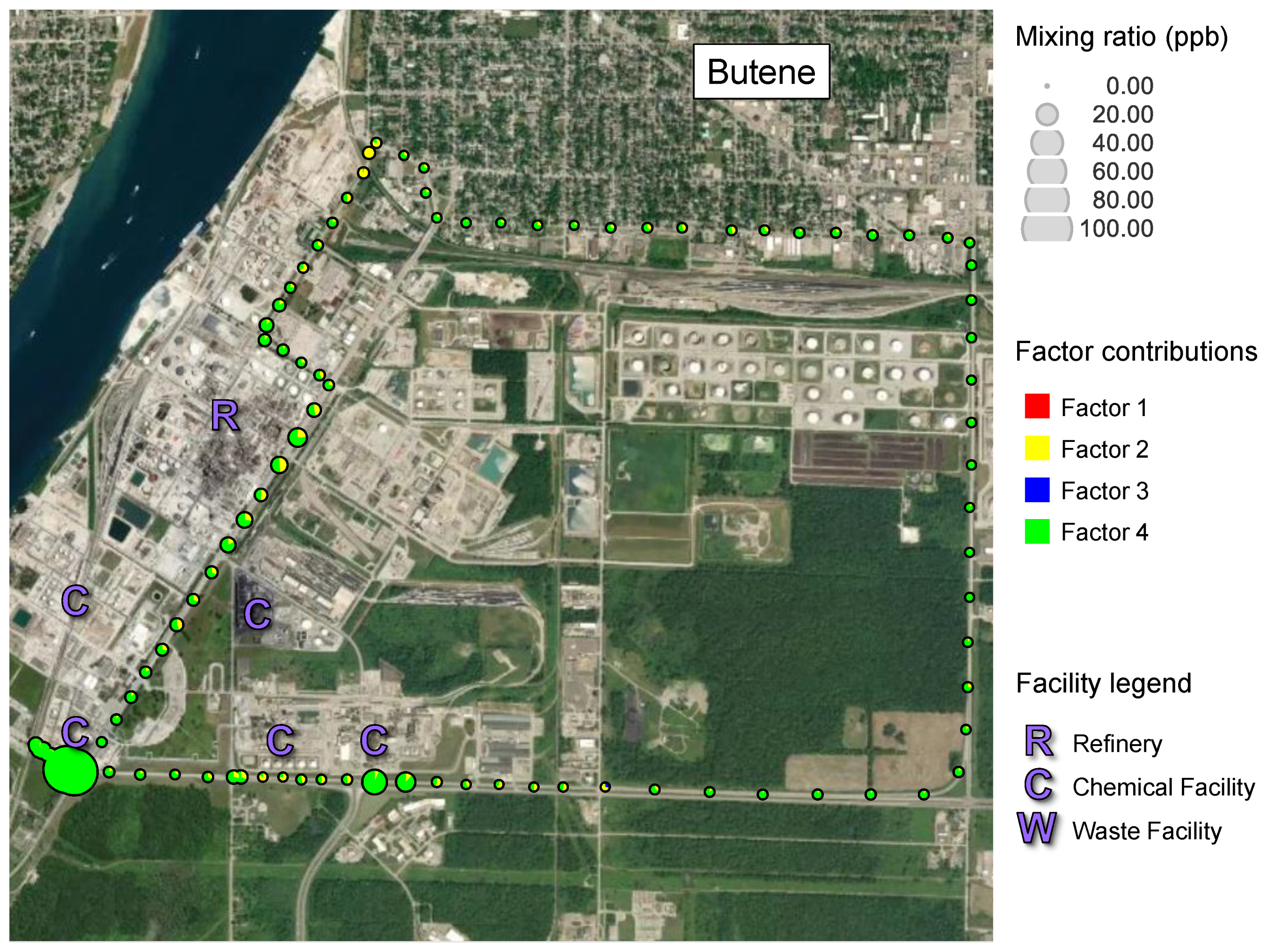
3.6. Spatially Resolved Apportionment: Butene
3.7. Overall Source Apportionment Results
4. Conclusions
Supplementary Materials
Author Contributions
Funding
Institutional Review Board Statement
Informed Consent Statement
Data Availability Statement
Acknowledgments
Conflicts of Interest
References
- Kansal, A. Sources and Reactivity of NMHCs and VOCs in the Atmosphere: A Review. J. Hazard. Mater. 2009, 166, 17–26. [Google Scholar] [CrossRef] [PubMed]
- McDonald, B.C.; de Gouw, J.A.; Gilman, J.B.; Jathar, S.H.; Akherati, A.; Cappa, C.D.; Jimenez, J.L.; Lee-Taylor, J.; Hayes, P.L.; McKeen, S.A.; et al. Volatile Chemical Products Emerging as Largest Petrochemical Source of Urban Organic Emissions. Science 2018, 359, 760. [Google Scholar] [CrossRef] [Green Version]
- Gkatzelis, G.I.; Coggon, M.M.; McDonald, B.C.; Peischl, J.; Aikin, K.C.; Gilman, J.B.; Trainer, M.; Warneke, C. Identifying Volatile Chemical Product Tracer Compounds in U.S. Cities. Environ. Sci. Technol. 2021, 55, 188–199. [Google Scholar] [CrossRef] [PubMed]
- Seinfeld, J.H.; Pandis, S.N. Atmospheric Chemistry and Physics: From Air Pollution to Climate Change; John Wiley & Sons: New York, NY, USA, 1998. [Google Scholar]
- Jia, C.; Batterman, S.; Godwin, C. VOCs in Industrial, Urban and Suburban Neighborhoods, Part 1: Indoor and Outdoor Concentrations, Variation, and Risk Drivers. Atmos. Environ. 2008, 42, 2083–2100. [Google Scholar] [CrossRef]
- Hallquist, M.; Wenger, J.C.; Baltensperger, U.; Rudich, Y.; Simpson, D.; Claeys, M.; Dommen, J.; Donahue, N.M.; George, C.; Goldstein, A.H.; et al. The Formation, Properties and Impact of Secondary Organic Aerosol: Current and Emerging Issues. Atmos. Chem. Phys. 2009, 9, 5155–5235. [Google Scholar] [CrossRef] [Green Version]
- Warneke, C.; Geiger, F.; Edwards, P.M.; Dube, W.; Pétron, G.; Kofler, J.; Zahn, A.; Brown, S.S.; Graus, M.; Gilman, J.B.; et al. Volatile Organic Compound Emissions from the Oil and Natural Gas Industry in the Uintah Basin, Utah: Oil and Gas Well Pad Emissions Compared to Ambient Air Composition. Atmos. Chem. Phys. 2014, 14, 10977–10988. [Google Scholar] [CrossRef] [Green Version]
- Liggio, J.; Li, S.-M.; Hayden, K.; Taha, Y.M.; Stroud, C.; Darlington, A.; Drollette, B.D.; Gordon, M.; Lee, P.; Liu, P.; et al. Oil Sands Operations as a Large Source of Secondary Organic Aerosols. Nature 2016, 534, 91–94. [Google Scholar] [CrossRef]
- USEPA Initial List of Hazardous Air Pollutants with Modifications. 2022. Available online: https://www.epa.gov/haps/initial-list-hazardous-air-pollutants-modifications (accessed on 19 October 2022).
- UNECE 1999 Protocol to Abate Acidification, Eutrophication and Ground-Level Ozone to the Convention on Long-Range Transboundary Air Pollution, as Amended on 4 May 2012. 2013. Available online: https://unece.org/environment-policy/air/protocol-abate-acidification-eutrophication-and-ground-level-ozone (accessed on 9 April 2021).
- ECCC Environment and Climate Change Canada 1990–2016 Air Pollutant Emission Inventory Report. 2016. Available online: https://publications.gc.ca/collections/collection_2018/eccc/en81-26-2016-eng.pdf (accessed on 13 April 2021).
- Miller, L.; Xu, X.; Luginaah, I. Spatial Variability of Volatile Organic Compound Concentrations in Sarnia, Ontario, Canada. J. Toxicol. Env. Health A 2009, 72, 610–624. [Google Scholar] [CrossRef]
- Stroud, C.A.; Zaganescu, C.; Chen, J.; McLinden, C.A.; Zhang, J.; Wang, D. Toxic Volatile Organic Air Pollutants across Canada: Multi-Year Concentration Trends, Regional Air Quality Modelling and Source Apportionment. J. Atmos. Chem. 2016, 73, 137–164. [Google Scholar] [CrossRef] [Green Version]
- Li, S.-M.; Leithead, A.; Moussa, S.G.; Liggio, J.; Moran, M.D.; Wang, D.; Hayden, K.; Darlington, A.; Gordon, M.; Staebler, R.; et al. Differences between Measured and Reported Volatile Organic Compound Emissions from Oil Sands Facilities in Alberta, Canada. Proc. Natl. Acad. Sci. USA 2017, 114, E3756. [Google Scholar] [CrossRef]
- Bari, M.A.; Kindzierski, W.B. Ambient Volatile Organic Compounds (VOCs) in Calgary, Alberta: Sources and Screening Health Risk Assessment. Sci. Total Environ. 2018, 631–632, 627–640. [Google Scholar] [CrossRef] [Green Version]
- Wren, S.N.; Mihele, C.M.; Lu, G.; Jiang, Z.; Wen, D.; Hayden, K.; Mittermeier, R.L.; Staebler, R.M.; Cober, S.G.; Brook, J.R. Improving Insights on Air Pollutant Mixtures and Their Origins by Enhancing Local Monitoring in an Area of Intensive Resource Development. Environ. Sci. Technol. 2020, 54, 14936–14945. [Google Scholar] [CrossRef]
- Xiong, Y.; Du, K. Source-Resolved Attribution of Ground-Level Ozone Formation Potential from VOC Emissions in Metropolitan Vancouver, BC. Sci. Total Environ. 2020, 721, 137698. [Google Scholar] [CrossRef]
- Xiong, Y.; Bari, M.A.; Xing, Z.; Du, K. Ambient Volatile Organic Compounds (VOCs) in Two Coastal Cities in Western Canada: Spatiotemporal Variation, Source Apportionment, and Health Risk Assessment. Sci. Total Environ. 2020, 706, 135970. [Google Scholar] [CrossRef]
- Paatero, P.; Tapper, U. Positive Matrix Factorisation- a Nonnegative Factor Model with Optmal Utilisation of Error-Estimates of Data Values. Environmetrics 1994, 5, 111–126. [Google Scholar] [CrossRef]
- Song, Y.; Shao, M.; Liu, Y.; Lu, S.; Kuster, W.; Goldan, P.; Xie, S. Source Apportionment of Ambient Volatile Organic Compounds in Beijing. Environ. Sci. Technol. 2007, 41, 4348–4353. [Google Scholar] [CrossRef]
- Vlasenko, A.; Slowik, J.G.; Bottenheim, J.W.; Brickell, P.C.; Chang, R.Y.-W.; Macdonald, A.M.; Shantz, N.C.; Sjostedt, S.J.; Wiebe, H.A.; Leaitch, W.R.; et al. Measurements of VOCs by Proton Transfer Reaction Mass Spectrometry at a Rural Ontario Site: Sources and Correlation to Aerosol Composition. J. Geophys. Res. Atmos. 2009, 114. [Google Scholar] [CrossRef] [Green Version]
- Bon, D.M.; Ulbrich, I.M.; de Gouw, J.A.; Warneke, C.; Kuster, W.C.; Alexander, M.L.; Baker, A.; Beyersdorf, A.J.; Blake, D.; Fall, R.; et al. Measurements of Volatile Organic Compounds at a Suburban Ground Site (T1) in Mexico City during the MILAGRO 2006 Campaign: Measurement Comparison, Emission Ratios, and Source Attribution. Atmos. Chem. Phys. 2011, 11, 2399–2421. [Google Scholar] [CrossRef] [Green Version]
- Yuan, B.; Shao, M.; de Gouw, J.; Parrish, D.D.; Lu, S.; Wang, M.; Zeng, L.; Zhang, Q.; Song, Y.; Zhang, J.; et al. Volatile Organic Compounds (VOCs) in Urban Air: How Chemistry Affects the Interpretation of Positive Matrix Factorization (PMF) Analysis. J. Geophys. Res. Atmos. 2012, 117, D24302. [Google Scholar] [CrossRef]
- Crippa, M.; Canonaco, F.; Slowik, J.G.; El Haddad, I.; DeCarlo, P.F.; Mohr, C.; Heringa, M.F.; Chirico, R.; Marchand, N.; Temime-Roussel, B.; et al. Primary and Secondary Organic Aerosol Origin by Combined Gas-Particle Phase Source Apportionment. Atmos. Chem. Phys. 2013, 13, 8411–8426. [Google Scholar] [CrossRef]
- McCarthy, M.C.; Aklilu, Y.-A.; Brown, S.G.; Lyder, D.A. Source Apportionment of Volatile Organic Compounds Measured in Edmonton, Alberta. Atmos. Environ. 2013, 81, 504–516. [Google Scholar] [CrossRef]
- Dumanoglu, Y.; Kara, M.; Altiok, H.; Odabasi, M.; Elbir, T.; Bayram, A. Spatial and Seasonal Variation and Source Apportionment of Volatile Organic Compounds (VOCs) in a Heavily Industrialized Region. Atmos. Environ. 2014, 98, 168–178. [Google Scholar] [CrossRef]
- Rocco, M.; Colomb, A.; Baray, J.-L.; Amelynck, C.; Verreyken, B.; Borbon, A.; Pichon, J.-M.; Bouvier, L.; Schoon, N.; Gros, V.; et al. Analysis of Volatile Organic Compounds during the OCTAVE Campaign: Sources and Distributions of Formaldehyde on Reunion Island. Atmosphere 2020, 11, 140. [Google Scholar] [CrossRef] [Green Version]
- Gkatzelis, G.I.; Coggon, M.M.; McDonald, B.C.; Peischl, J.; Gilman, J.B.; Aikin, K.C.; Robinson, M.A.; Canonaco, F.; Prevot, A.S.H.; Trainer, M.; et al. Observations Confirm That Volatile Chemical Products Are a Major Source of Petrochemical Emissions in U.S. Cities. Environ. Sci. Technol. 2021, 55, 4332–4343. [Google Scholar] [CrossRef] [PubMed]
- ECCC Environment and Climate Change Canada National Pollutant Release Inventory. 2019. Available online: https://www.canada.ca/en/environment-climate-change/services/national-pollutant-release-inventory/tools-resources-data/access.html (accessed on 13 April 2021).
- Oiamo, T.H.; Luginaah, I.N.; Atari, D.O.; Gorey, K.M. Air Pollution and General Practitioner Access and Utilization: A Population Based Study in Sarnia, “Chemical Valley,” Ontario. Environ. Health 2011, 10, 71. [Google Scholar] [CrossRef] [Green Version]
- Jordan, A.; Haidacher, S.; Hanel, G.; Hartungen, E.; Märk, L.; Seehauser, H.; Schottkowsky, R.; Sulzer, P.; Märk, T.D. A High Resolution and High Sensitivity Proton-Transfer-Reaction Time-of-Flight Mass Spectrometer (PTR-TOF-MS). Int. J. Mass Spectrom. 2009, 286, 122–128. [Google Scholar] [CrossRef]
- Baudic, A.; Gros, V.; Sauvage, S.; Locoge, N.; Sanchez, O.; Sarda-Estève, R.; Kalogridis, C.; Petit, J.-E.; Bonnaire, N.; Baisnée, D.; et al. Seasonal Variability and Source Apportionment of Volatile Organic Compounds (VOCs) in the Paris Megacity (France). Atmos. Chem. Phys. 2016, 16, 11961–11989. [Google Scholar] [CrossRef] [Green Version]
- Wang, L.; Slowik, J.G.; Tripathi, N.; Bhattu, D.; Rai, P.; Kumar, V.; Vats, P.; Satish, R.; Baltensperger, U.; Ganguly, D.; et al. Source Characterization of Volatile Organic Compounds Measured by Proton-Transfer-Reaction Time-of-Flight Mass Spectrometers in Delhi, India. Atmos. Chem. Phys. 2020, 20, 9753–9770. [Google Scholar] [CrossRef]
- Li, H.; Canagaratna, M.R.; Riva, M.; Rantala, P.; Zhang, Y.; Thomas, S.; Heikkinen, L.; Flaud, P.-M.; Villenave, E.; Perraudin, E.; et al. Atmospheric Organic Vapors in Two European Pine Forests Measured by a Vocus PTR-TOF: Insights into Monoterpene and Sesquiterpene Oxidation Processes. Atmos. Chem. Phys. 2021, 21, 4123–4147. [Google Scholar] [CrossRef]
- Tan, Y.; Han, S.; Chen, Y.; Zhang, Z.; Li, H.; Li, W.; Yuan, Q.; Li, X.; Wang, T.; Lee, S. Characteristics and Source Apportionment of Volatile Organic Compounds (VOCs) at a Coastal Site in Hong Kong. Sci. Total Environ. 2021, 777, 146241. [Google Scholar] [CrossRef]
- Yang, Y.; Liu, B.; Hua, J.; Yang, T.; Dai, Q.; Wu, J.; Feng, Y.; Hopke, P.K. Global Review of Source Apportionment of Volatile Organic Compounds Based on Highly Time-Resolved Data from 2015 to 2021. Environ. Int. 2022, 165, 107330. [Google Scholar] [CrossRef]
- Majluf, F.Y.; Krechmer, J.E.; Daube, C.; Knighton, W.B.; Dyroff, C.; Lambe, A.T.; Fortner, E.C.; Yacovitch, T.I.; Roscioli, J.R.; Herndon, S.C.; et al. Mobile Near-Field Measurements of Biomass Burning Volatile Organic Compounds: Emission Ratios and Factor Analysis. Environ. Sci. Technol. Lett. 2022, 9, 383–390. [Google Scholar] [CrossRef]
- Norris, G.; Duvall, R.; Brown, S.; Bai, S. EPA Positive Matrix Factorization (PMF) 5.0 Fundamentals and User Guide. 2014. Available online: https://www.epa.gov/sites/default/files/2015-02/documents/pmf_5.0_user_guide.pdf (accessed on 15 July 2022).
- Paatero, P. The Multilinear Engine-a Table-Driven, Least Squares Program for Solving Multilinear Problems, Including the n-Way Parallel Factor Analysis Model. J. Comput. Graph. Stat. 1999, 8, 854–888. [Google Scholar]
- Slowik, J.G.; Vlasenko, A.; McGuire, M.; Evans, G.J.; Abbatt, J.P.D. Simultaneous Factor Analysis of Organic Particle and Gas Mass Spectra: AMS and PTR-MS Measurements at an Urban Site. Atmos. Chem. Phys. 2010, 10, 1969–1988. [Google Scholar] [CrossRef] [Green Version]
- Sofowote, U.M.; Su, Y.; Dabek-Zlotorzynska, E.; Rastogi, A.K.; Brook, J.; Hopke, P.K. Constraining the Factor Analytical Solutions Obtained from Multiple-Year Receptor Modeling of Ambient PM2.5 Data from Five Speciation Sites in Ontario, Canada. Atmos. Environ. 2015, 108, 151–157. [Google Scholar] [CrossRef]
- Gueneron, M.; Erickson, M.H.; VanderSchelden, G.S.; Jobson, B.T. PTR-MS Fragmentation Patterns of Gasoline Hydrocarbons. Int. J. Mass Spectrom. 2015, 379, 97–109. [Google Scholar] [CrossRef]
- Erickson, M.H.; Gueneron, M.; Jobson, B.T. Measuring Long Chain Alkanes in Diesel Engine Exhaust by Thermal Desorption PTR-MS. Atmos. Meas. Tech. 2014, 7, 225–239. [Google Scholar] [CrossRef] [Green Version]
- Healy, R.M.; Chen, Q.; Bennett, J.; Karellas, N.S. A Multi-Year Study of VOC Emissions at a Chemical Waste Disposal Facility Using Mobile APCI-MS and LPCI-MS Instruments. Environ. Pollut. 2017, 232, 220–228. [Google Scholar] [CrossRef]
- ECCC Environment and Climate Change Canada National Air Pollution Surveillance Program. 2022. Available online: https://www.canada.ca/en/environment-climate-change/services/air-pollution/monitoring-networks-data/national-air-pollution-program.html (accessed on 6 July 2022).
- Ashbaugh, L.L.; Malm, W.C.; Sadeh, W.Z. A Residence Time Probability Analysis of Sulfur Concentrations at Grand Canyon National Park. Atmos. Environ. (1967) 1985, 19, 1263–1270. [Google Scholar] [CrossRef]
- Verreyken, B.; Amelynck, C.; Schoon, N.; Müller, J.-F.; Brioude, J.; Kumps, N.; Hermans, C.; Metzger, J.-M.; Colomb, A.; Stavrakou, T. Measurement Report: Source Apportionment of Volatile Organic Compounds at the Remote High-Altitude Maïdo Observatory. Atmos. Chem. Phys. 2021, 21, 12965–12988. [Google Scholar] [CrossRef]
- Read, K.A.; Carpenter, L.J.; Arnold, S.R.; Beale, R.; Nightingale, P.D.; Hopkins, J.R.; Lewis, A.C.; Lee, J.D.; Mendes, L.; Pickering, S.J. Multiannual Observations of Acetone, Methanol, and Acetaldehyde in Remote Tropical Atlantic Air: Implications for Atmospheric OVOC Budgets and Oxidative Capacity. Environ. Sci. Technol. 2012, 46, 11028–11039. [Google Scholar] [CrossRef] [PubMed]
- Loomis, D.; Guyton, K.Z.; Grosse, Y.; El Ghissassi, F.; Bouvard, V.; Benbrahim-Tallaa, L.; Guha, N.; Vilahur, N.; Mattock, H.; Straif, K. Carcinogenicity of Benzene. Lancet Oncol. 2017, 18, 1574–1575. [Google Scholar] [CrossRef]


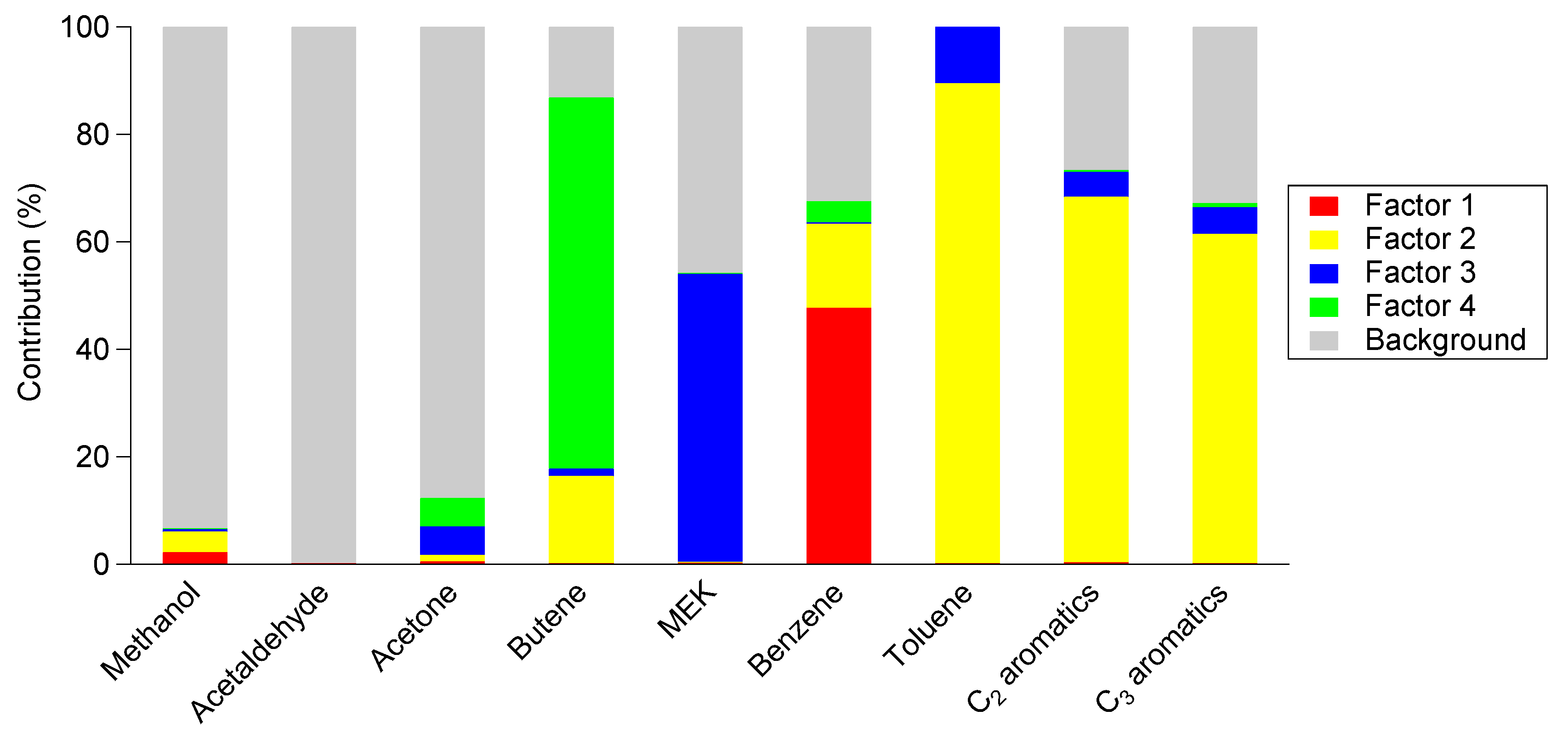
| Factor 1 | Factor 2 | Factor 3 | Factor 4 | Background | |
|---|---|---|---|---|---|
| Methanol | 2.2 | 3.9 | 0.4 | 0.0 | 93.5 |
| Acetaldehyde | 0.0 | 0.0 | 0.0 | 0.0 | 100.0 |
| Acetone | 0.5 | 1.2 | 5.3 | 5.2 | 87.7 |
| Butene | 0.0 | 16.4 | 1.4 | 69.1 | 13.1 |
| MEK | 0.2 | 0.0 | 53.8 | 0.2 | 45.8 |
| Benzene | 47.7 | 15.7 | 0.1 | 4.1 | 32.5 |
| Toluene | 0.1 | 89.4 | 10.5 | 0.0 | 0.0 |
| C2 aromatics | 0.3 | 68.0 | 4.6 | 0.4 | 26.6 |
| C3 aromatics | 0.2 | 61.3 | 5.0 | 0.8 | 32.8 |
Publisher’s Note: MDPI stays neutral with regard to jurisdictional claims in published maps and institutional affiliations. |
© 2022 by the authors. Licensee MDPI, Basel, Switzerland. This article is an open access article distributed under the terms and conditions of the Creative Commons Attribution (CC BY) license (https://creativecommons.org/licenses/by/4.0/).
Share and Cite
Healy, R.M.; Sofowote, U.M.; Wang, J.M.; Chen, Q.; Todd, A. Spatially Resolved Source Apportionment of Industrial VOCs Using a Mobile Monitoring Platform. Atmosphere 2022, 13, 1722. https://doi.org/10.3390/atmos13101722
Healy RM, Sofowote UM, Wang JM, Chen Q, Todd A. Spatially Resolved Source Apportionment of Industrial VOCs Using a Mobile Monitoring Platform. Atmosphere. 2022; 13(10):1722. https://doi.org/10.3390/atmos13101722
Chicago/Turabian StyleHealy, Robert M., Uwayemi M. Sofowote, Jonathan M. Wang, Qingfeng Chen, and Aaron Todd. 2022. "Spatially Resolved Source Apportionment of Industrial VOCs Using a Mobile Monitoring Platform" Atmosphere 13, no. 10: 1722. https://doi.org/10.3390/atmos13101722