Routes Alternatives with Reduced Emissions: Large-Scale Statistical Analysis of Probe Vehicle Data in Lyon

Abstract

Vehicle air pollution is a significant problem for health and climate change that can be solved by several approaches. The route is one of the many components to be considered. In this work, we propose a statistical analysis of a large FCD database in November 2017 in Lyon (France) in order to find alternative sustainable trips and evaluate potential emission reductions (CO₂, NOx, PM10). To this end, an innovative framework was built. First, we assessed vehicle speeds for each network section and the fifteen-minute period, when this information was reachable. Then, we used a regression random forest (RF) algorithm to fill in the missing data. This dynamical speed map allowed us to search for fewer pollutant trips, for the first ten days of November. By using COPERT emission factors (EFs) and the time-dependent Dijkstra algorithm, we successfully identified between 51% and 72% of alternative sustainable paths, depending on the engine technology and the pollutant. We investigated the influence of vehicle technology. In all cases, the number of alternative trips found tends to be the same as soon as the emission savings exceed 5%. Moreover, about 400 trips out of 11,000 have the potential to mitigate about 20% of emissions.

1. Introduction

1.1. General Information and Background

Many studies have shown that ambient air pollution has a significant impact on health [1,2], environment [3,4,5], and climate change [6,7]. Air pollutants can be discriminated into global pollutants such as CO₂ and O₃, GHG impacting the Earth’s climate, and local pollutants like NO_x, PM, and SO₂, affecting the health of the population. Both can damage the environment. In 2016, the WHO estimated that three million people die each year from air pollution worldwide [8]. Although COVID-19 has led to a different paradigm for governments, companies, and workers with more and more telework, road traffic is still among the largest contributors to ambient air pollution, especially in urban environments. Thus, road transport is a fundamental challenge in the combat against air pollution, and many studies have been carried out to assess urban traffic emissions [9,10].

Traffic-related emissions may be assessed at the microscopic (vehicle, high temporal resolution) and macroscopic (fleets of vehicles, time slots of a few minutes) scales. The microscopic scale seems more accurate with models such as PHEM [11,12], CMEM [13], and CRUISE [14], which provide efficient instantaneous emissions from parameters such as speed, acceleration, and engine characteristics. Nevertheless, this approach requires high-precision data and leads to long computational times which is adequate for very localized areas but inappropriate on a large urban scale [15,16]. On the other hand, the macroscopic method is suitable and widely used to assess traffic emissions on this scale with only two traffic variables as inputs (average travel speed (TS; abbreviations were summarized in Table S1) and the corresponding travel distance (TD)). Among macroscopic emission models such as ARTEMIS [17] and HBEFA [18], COPERT [19] appears to be an efficient model for estimating traffic-related emissions on the urban scale in Europe, considering vehicle fleet distribution and vehicle emission rates [16,20]. These microscopic and macroscopic models are either embedded in traffic simulation models or applied to real-world data such as loops, sensors, and GPS traces from navigation systems.

In the early 2000s, GPS data mining was used increasingly in two research domains: transportation science investigating personal and vehicle trips, and human geography exploring the relationship between people, places, and the environment [21]. In transportation, GPS-based data are mainly employed for studying urban mobility patterns [22,23], intelligent transportation systems [24,25], traffic state estimation, and prediction [26,27]. However, there are some limitations such as missing data (e.g., GPS signals blocked in underground sites), interference near high-rise buildings, positions of the road network, and noise (e.g., journey detours, GPS device switch-off delay) [28,29]. Nevertheless, GPS traces characterize trips better than static sensors, such as loops. They provide an excellent resolution for tracking a vehicle’s position at a large scale compared to mobile data. Moreover, they cover the urban road network well with excellent spatial and temporal distribution, and they are representative of the entire vehicle fleet, providing real-world daily trajectories. Consequently, GPS data accurately estimate vehicle speeds on network links, thus mean speed flows and their variation along the day. Previous studies suggest that penetration rates should be higher than 20% to guarantee accurate speed estimation over links in an urban road network [30]. This type of data provides valuable information for emissions assessments, especially using COPERT model.

1.2. Literature Review

The main idea behind eco-routing is to find a path from an origin to a destination (OD), consuming less fuel and/or emitting less pollutants for a vehicle. Although common sense entails thinking in terms of the shortest path (SP) or the fastest path (FP), some studies have shown that the optimal trips considering environmental objectives do not always correspond to these paths, especially at lower congested speeds [31,32,33]. Different approaches to find an eco-friendly path have been investigated with traffic data using either simulation traffic models [32,34,35] or real-world data [33,36,37,38,39,40] combined with a microscopic [32,34] or macroscopic [41,42] emission model.

The eco-routing methods developed in traffic simulations provide much helpful network-wide information. In particular, they can study many trips considering emission and fuel consumption (FC) for diverse vehicle populations. For instance, Ahn et Rakha [32] and Guo et al. [42] explored the impact of market penetration of eco-routing systems on network-wide performance. By implementing the INTEGRATION software including the VT-Micro microscopic emission model, Ahn et Rakha found that the benefits of using an eco-routing system tended to increase with its level of market penetration. Using TRANSIMS with MOVES, Guo et al. found significant sustainable benefits could be obtained at low penetration rates of targeted eco-routing strategies. Indeed, nearly half of emission reductions can be obtained at 10% of targeted market penetration, and most emission reductions at 40%. Combining VISSIM and a microscopic emission model based on vehicle-specific power (VSP), Bandeira et al. [43] discovered that UE eco-routing might cause opposite effects at the network scale. Nonetheless, the trade-off between emissions and travel time (TT) can generally be minimized with adequate routing strategies. Wang et al. [35] proposed a time-dependent eco-routing method with INTEGRATION and VT-CPFM, producing lower network-wide energy consumption levels than the ECO-AFA and TT-AFA eco-routing developed previously [32,44].

The eco-routing methods developed with experimental data rely on (i) traffic measurements (loops, sensors, GPS, etc.) (ii) emission measurements (on-road emission measurements (OEMs), and portable emission measurement system (PEMS)). The latter are on-board devices installed in vehicles collecting accurate driving information in real road situations in a study framework. On-board devices have often been used in eco-routing research because of their convenience for directly logging geolocated vehicle information such as velocity, acceleration, FC, and pollutant emissions. Ericsson et al. [36] proposed a method using two microscopic FC models directly related to CO₂ emissions (VETO and VeTESS) on a GPS probe dataset gathered by 284 vehicles over ten months in the framework of an intelligent speed adaptation trial in Lund (Sweden). They worked with ArcGIS and its network analysis module based on the Dijkstra algorithm [45] to provide a static alternative route to first reduce the fuel consumption of an actual trip and then an alternative route considering traffic disturbance to produce a dynamic route guidance system. However, despite the extensive data available in a medium-sized area of 27 km² with 2232 links, they conducted only a few trips because they had to deal with complex preprocessing operations due to the structure of the database, such as detours and short or incomplete journeys. Moreover, although they exploited microscopic models to produce their FC factors, the latter turned out to be significant range aggregated factors, with penalties added only for the dynamic route guidance part. Yao et Song [38] utilized data collection by PEMS to establish their emission and FC models based on a microscopic emission model (VSP) coupled with an aggregation process. Referring to the research of Lin et al. [46], they combined road traffic information from a probe vehicle system with a historical database to create a dynamic TT information database updated every five minutes. Then, they proposed a dynamic eco-routing method with a time-dependent Dijkstra algorithm and the same database. However, the link speed estimation formulated by Lin et al. [46] is a rough nationwide method poorly adapted to producing dynamic information in five-minute intervals. Additionally, they did not describe the probe vehicle system used, and they assessed their eco-routing process on random simulated OD instead of actual OD. Zeng et al. worked with a ten-month range of 153 probe vehicles data in Toyota city (Japan) to predict FC with a support vector machine (SVM) first [47], and then vehicle CO₂ emissions for eco-routing navigation [33,39,40]. Probe vehicles have been equipped with On-board GPS and controller area network (CAN) devices to provide geolocated information such as speed, acceleration, and FC. In 2015, they combined vehicle dynamics theory with CAN data to estimate FC, CO₂ emissions, and TT at the link-based level [33]. In 2017, they trained an SVM machine learning method with these link-based CO₂ emissions estimated to predict CO₂ emissions for each link directly [37]. Finally, both studies modelled the transportation network composed of 12,877 links as a directed graph on which they built a static eco-routing method with the Dijkstra algorithm, a constraint on TT, and k-SPs. The first minimized a combination of TT and CO₂ emissions to find the sustainable path (SuP) along the Pareto frontier with CAN data. Missing observations were filled by weighted data from neighboring links, while the second was deduced with the SVM model. The eco-path was calculated for each of them under various TT constraints. The authors conducted a sensitivity analysis based on almost 8000 real-world trips recorded for one month. In 2020, they updated their previous work with a new vehicle dynamics theory and a new eco-routing model based on a Lagrangian relaxation approach instead of using the Pareto frontier considering a specified TT budget given an on-time arrival probability [40]. Nevertheless, for all their studies presented above, and assumed for the one in 2020, they filled in missing data on network links by a simple method considering the weight of the neighboring links to tackle data sparsity. Moreover, they built a static model, with a one-month TT and emissions aggregated at the link-based level, which is sizable enough to take congestion into account during peak hours and an approximate traffic state. Additionally, they proposed only an eco-routing method based on FC and CO₂ emission without sampling the vehicle engine through a TT constraint.

1.3. Research Questions

Policymakers want to encourage people to take less polluting routes. In France, this desire was reinforced in August 2022 by the adoption of measures requiring mobility applications to provide environmental information to users. In this context, the objective of this paper is to assess the potential for emissions savings from sustainable alternative route finding at the urban scale through a large database of GPS tracks. From a methodological viewpoint, simulation traffic models are attractive tools for carrying out large-scale studies. Still, they may be less representative of the real world than GPS-based trajectories. Indeed, GPS-based vehicle data seem to be the relevant choice to consider eco-routing problems since the objective is to offer an eco-friendly path for actual trajectories [34]. In addition, OEMs and PEMS are costly and provide only limited data to the test vehicles involved in data collection. Assessing emissions instead of measuring directly enables applying and comparing a mean EF (related to a global fleet) to a specific one (related to a specific engine).

In a nutshell, many studies have already explored eco-routing with GPS probe data in the framework of experimental research. Thus, the GPS-based studies were limited by the number of vehicles studied (284 vehicles for Ericsson et al. [36]; 153 vehicles for Zeng et al. [33,39,40]). However, to the authors’ knowledge, there is a lack of eco-routing studies with a large database of GPS traces, which are now readily available with technological advances. Moreover, eco-routing research based on GPS data, even with a large database, is challenging due to missing data which prevents building reliable traffic states for an entire network. Due to this limitation, most of these studies (i) have focused on a part of the network, and (ii) compromised fine temporal resolution. Thus, the aggregation of traffic variables such as speed over a significant time range leads, on the one hand, to poor consideration of congestion and, on the other hand, to a reduction in the accuracy of the time-dependent method. Moreover, most studies have compared their eco-routing process to the SP or the FP instead of the actual trajectory recorded, thus failing to assess the gains of eco-routing compared to the actual trajectories. Finally, eco-friendly path research is mainly based on FC, directly related to CO₂ emissions. Nonetheless, local pollutants such as NOx and PM are often not investigated.

Consequently, this study proposes an innovative approach to efficiently explore a large GPS trace database from a large vehicle fleet at the urban scale to find a sustainable alternative route to that taken. We explore methods to refresh traffic information every fifteen minutes from the GPS database, thereby allowing us to finely describe congestion. Thus, we use a macroscopic emission model, COPERT, to investigate many actual trajectories, looking for sustainable alternative routes and taking into account both global and local pollutants. We also assess the gains of eco-routing compared to the actual trajectories. Consequently, we ask the following questions: What are the challenges of eco-routing seen through the scope of GPS trajectories? From the perspective of air pollution, how many trips have alternatives with lower emissions inside our dataset? How much can we save on emissions and FC at the individual level? What is the magnitude of these gains regarding OD, pollutant, and vehicle type? Can we define a multi-pollutant criterion when looking for trip alternatives? The remainder of this article is structured as follows. Section 2 provides a description of the study site, data collection and preparation, and the eco-routing methods used for this research. Then, in Section 3 we describe the results and statistical analyses. Afterward, in Section 4, we discuss the main results of the study. Finally, Section 4 provides the conclusion in which perspectives are given according to the results.

2. Materials and Methods

2.1. Data Presentation

2.1.1. General Characteristics

We worked on an extensive GPS dataset from FCD, gathered by the company MediaMobile between 1 October 2017, and 30 September 2018, as part of the “Spot2Park” project. They extracted road traffic data for the Lyon urban area from various navigation system technologies installed in a large number of floating vehicles. The road network in their study area comprises a total of 319,590 links.

Each link has a unique ID assigned with several features provided, such as length, free-flow speed (ffs), speed limit, functional road class (frc), the form of way (fow), the relevance in the network (netclass), and 2D geometry. Each GPS user also has a unique user ID for which each position is stored, giving positions with a timestamp associated. Then, MediaMobile projected raw GPS positions on the links road network, and each user ID was processed with their path links. Finally, they inferred vehicle speed, coverage, and thus the entrance timestamp on each link traveled for each user based on projected GPS traces. Several billion observations on road networks were inferred for that period, including 383 million for November 2017.

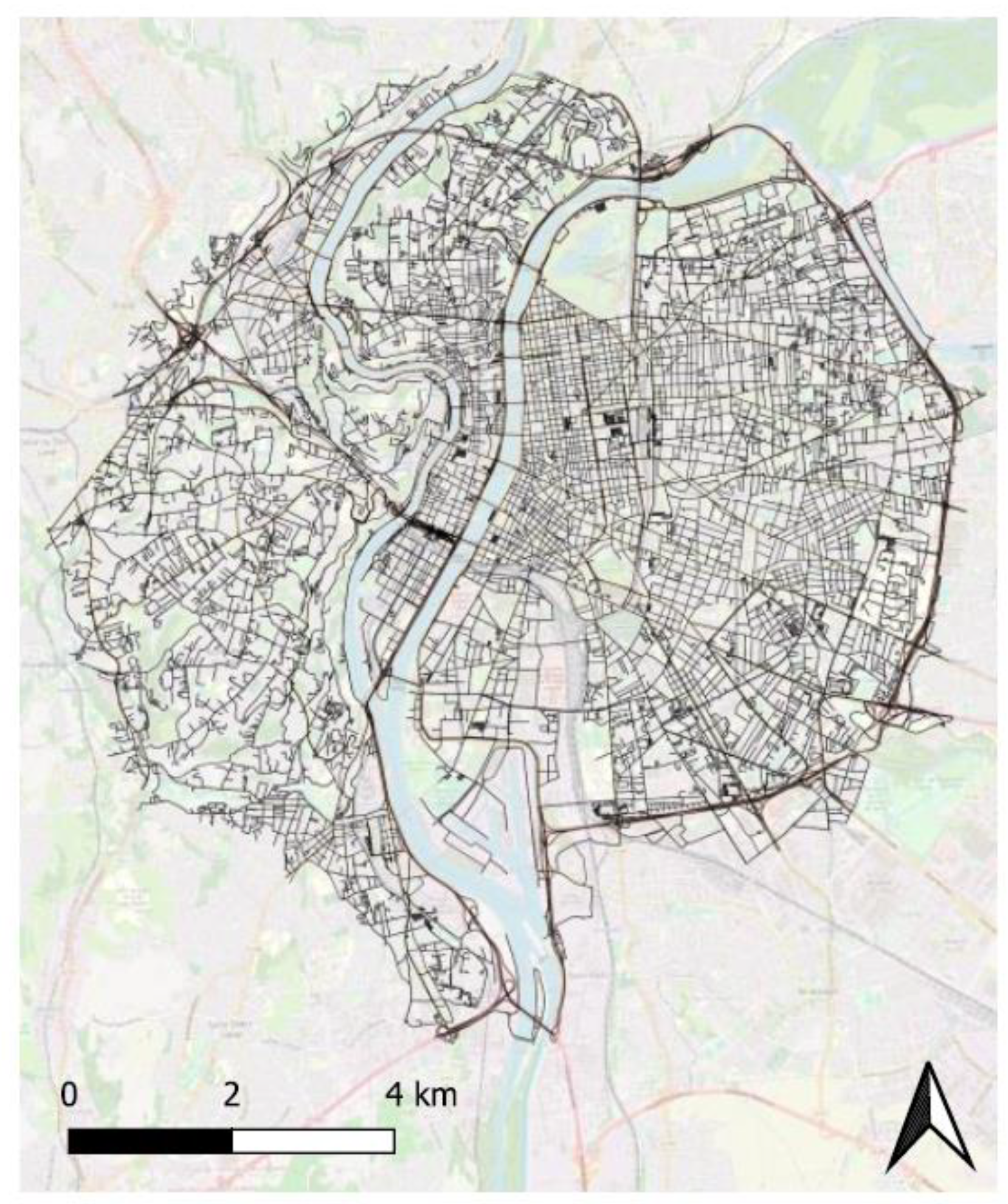
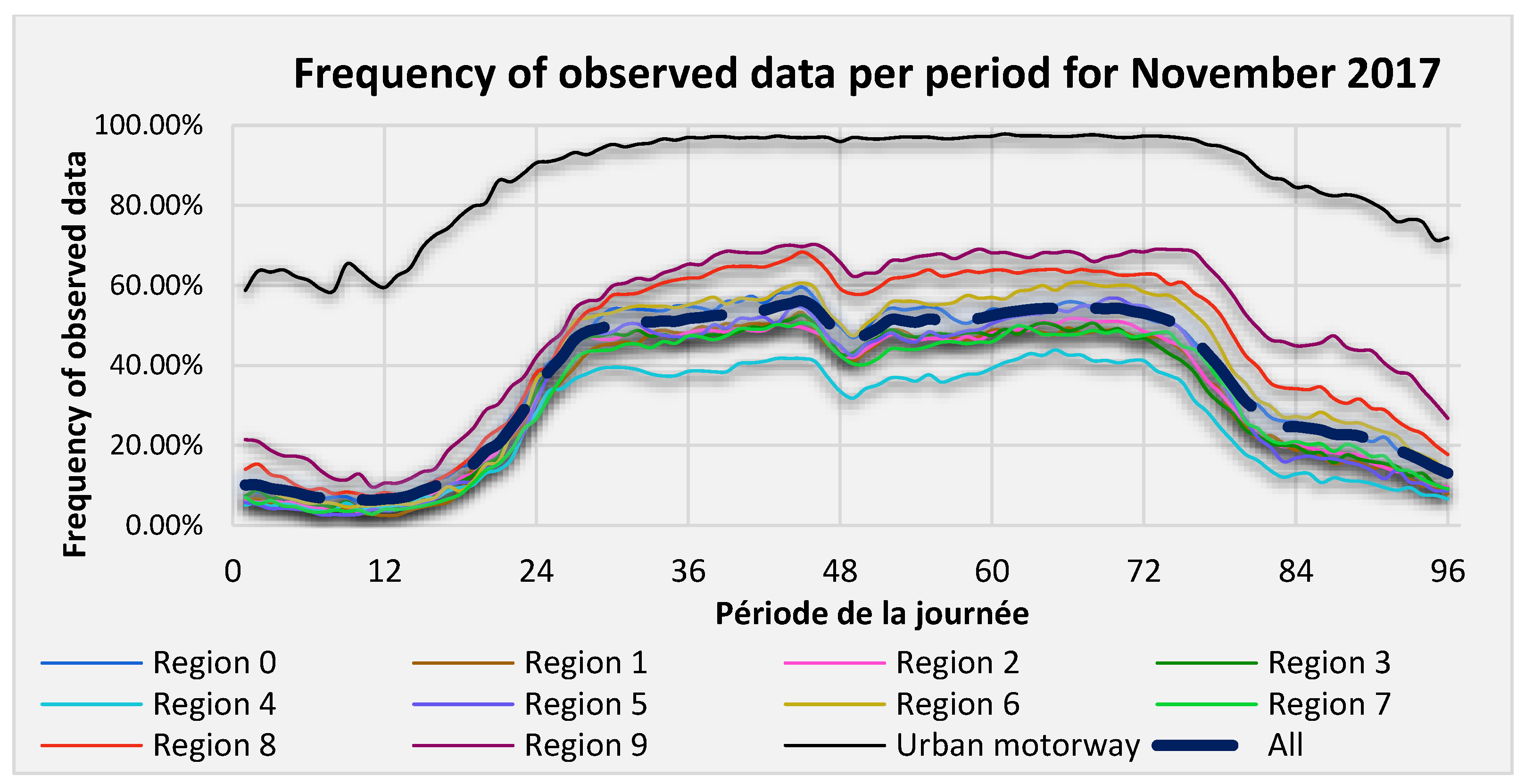
2.1.2. Geographic Site

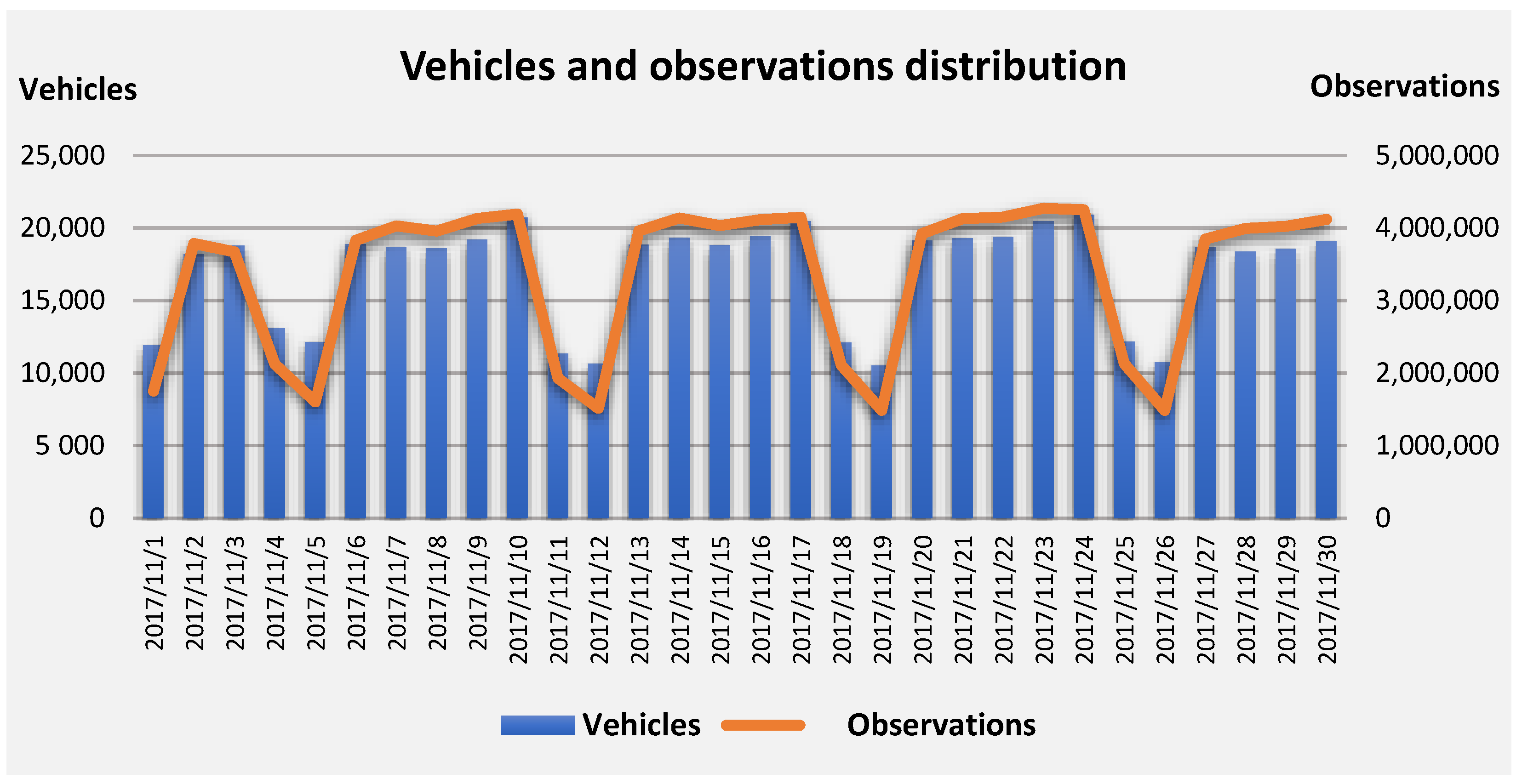
We chose to limit our study to the city of Lyon and its neighboring suburbs (Villeurbanne, Caluire, etc.), which had 960,036 inhabitants in 2017 [48]. As a result, the area investigated, shown in Figure 1, presents a surface area of almost 100 km² containing 39,812 links for a total length of 2264 km.

2.1.3. Data Studied

Due to a large amount of data, we chose to limit our study temporally to November 2017, in addition to the spatial limit. The period studied was chosen to anticipate the need for researching low-emission alternative trips and to obtain a valuable and large dataset to train the RF. Indeed, this period is characterized by few school holidays and an amount of available data similar for each week outside school holidays. The temporal restriction led to working with one hundred million raw observations for 508,373 vehicles, distributed according to each day of November 2017, as shown in Figure 2. The average number of vehicles is 16,946 per day. In 2017, the traffic fleet was composed of 87% of passenger cars of which 57% used diesel and 42% used petrol, 11.5% of light commercial vehicles, 1% of heavy-duty trucks, and 0.5% of public transport [49]. Moreover, the average speed in the network was about 30 km/h in November 2017. The road has the common characteristics of urban roads.

In this spatiotemporal framework, the speed limits ranged from 30 km/h to 110 km/h. Links are classified into 8 classes depending on their importance in the network. The definition and distribution of link categories are presented in Table S2 and Figure S1 in Supplementary Materials. Moreover, connections between links near a bridge or tunnel are checked [50] and enhanced, including virtual altimetry to avoid impossible routing for the implementation of the trip enhancement method and alternative trips research.

2.2. Experimental Protocol

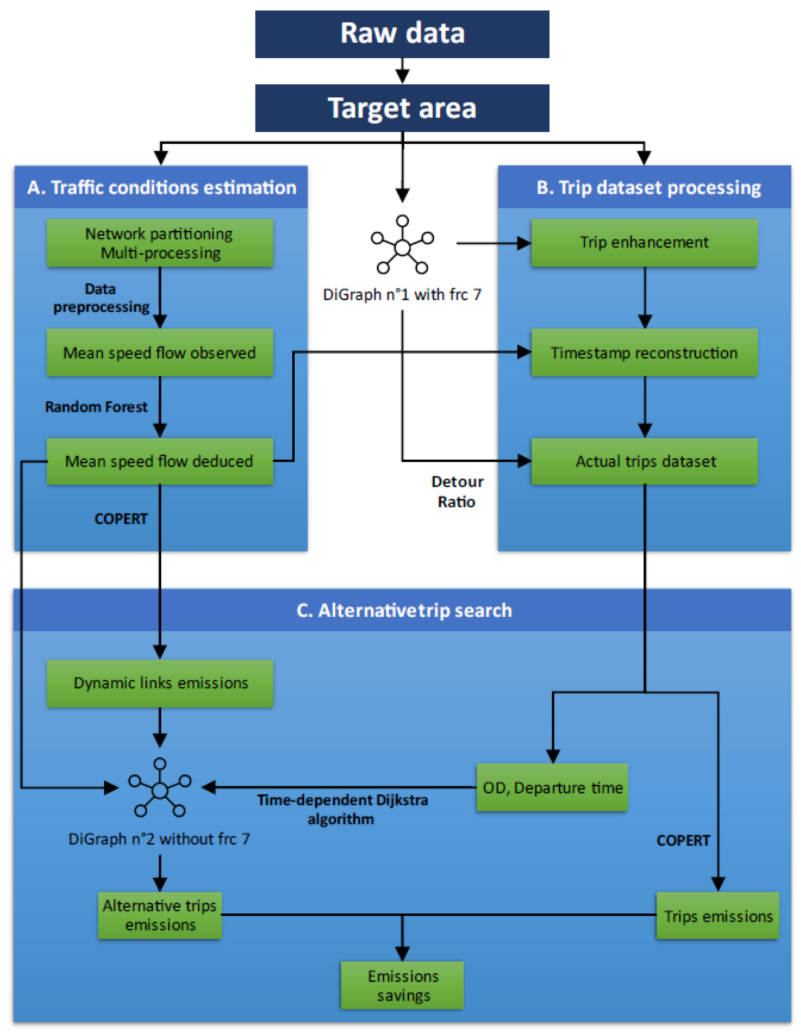
2.2.1. Overview

The main principle of the proposed eco-routing method is that a dynamic network, constructed on the basis of abundant FCD and providing traffic states every fifteen minutes, can be an efficient tool to find a path emitting fewer air pollutants. Nevertheless, the eco-routing method must conform to one rule: to avoid roads of minor importance because these roads have not been dimensioned to deal with re-routed vehicles. Indeed, our method is not meant to cause additional environmental externalities for local roads. Moreover, we do not address road grades, weather, or acceleration to estimate pollutant emissions. Our research focuses on a sustainable alternative path; thus, traffic condition is assumed to be stable, which means there is no change in traffic due to the route changes.

The methodological framework is outlined as follows:

A

A supervised machine learning method is proposed to reconstitute traffic conditions in fifteen-minute intervals over all network links based on FCD observations;

B

A trip dataset processing is performed on trips with spatiotemporal gaps to maintain the original pattern of actual trips and increase the sampling frequency;

C

Time-dependent searching of eco-friendly trips is carried out for every OD of the preserved actual trips, optimizing one pollutant or multi-pollutants.

The primary scientific hurdle is to establish every fifteen minutes, from the partial data, an estimate of the traffic conditions on the network elements for which there was no information (mainly the average speeds practiced on each link). The idea behind the aggregation of fifteen minutes is, on the one hand, to minimize missing data, and on the other hand, to consider the temporal similitude while preserving the dynamics of network information, notably during peak hours. To this end, the road network is partitioned into eleven regions to parallelize the process. Then, a random forest regression is trained with the observed average speed of the links as a target to capture spatiotemporal network features and infer the missing average speeds region by region [51,52].

The secondary barrier to be raised is to construct a reliable trip dataset. To do this, our study attempted to tackle spatial and temporal discontinuities for certain observed trips. Indeed, because of the FCD structure, trips may display spatial or/and temporal deficiencies requiring processing to conserve the journey of the vehicle concerned. Thus, some discontinuous trips are enhanced spatially with a directed and weighted road network graph on which the Dijkstra algorithm is performed, inspired by the trip enrichment method of Papuiri et al. [53]. Then, the timestamps of the inputs and outputs of the links are reconstructed with the observed and inferred average speed of network links. Only actual trips for which a sustainably alternative trip makes sense are preserved for examination. This was performed on the basis of the detour ratio ($DR$) principle (cf. 2.2.3.2), i.e., the ratio of the actual driving distance to the corresponding Euclidean distance or the SP, and visual control.

Finally, the last purpose is to implement a method for seeking eco-friendly trips and evaluating pollutant emissions in order to estimate emission savings. Directed Graphs (DiGraphs) of the road network are built for each pollutant or multi-pollutants. These DiGraphs are composed of nodes and edges. Edges represent road links and may store helpful information, such as pollutant emissions, average speed, link length, etc. To investigate alternative eco-friendly paths, pollutant emissions are estimated for each interval of fifteen minutes with a COPERT macroscopic emission model based on the average link speed in the inputs. This information is supplied to every edge in the DiGraphs, and the SP with link emissions as weights is computed. The TT on the links is also stored on every edge to update the weight of emissions for the application of the dynamic method.

The methodological framework is illustrated in Figure 3 below.

2.2.2. Traffic Condition Estimation

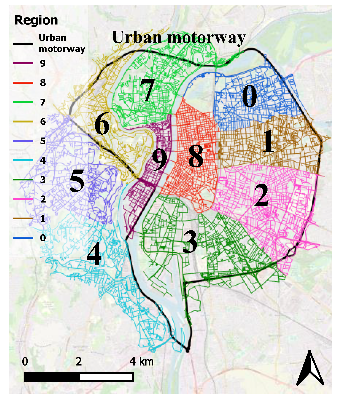
Network Partitioning

The site studied was divided into eleven distinct regions, including the Lyon urban motorway, to parallelize the machine learning process later. Figure 4 shows the result of the network partitioning process.

Data Preprocessing

Data preprocessing consists of the two following points in view to obtaining the input data required for the RF algorithm:

• The mean speed flow is computed at a specific temporal scale for each link where vehicles are observed;
• A matrix is prepared that combines features and average link speed flow as the observed or missing target.

In this study, we want to take traffic conditions and their evolution into consideration from real network information for the eco-routing problem. Nevertheless, we have to consider that, despite the extensive data available, the more we want to reflect changing traffic conditions accurately, the more we have to face the scarcity of data. Indeed, there is a lower bound for the time interval where the missing data just becomes too numerous because there is no observation in the dataset. For a 5 min interval, there are 157,421,682 missing data out of 196,957,440 expected data, i.e., about 80% of missing data. This is simply too much for any imputation algorithm. The 15 min interval leads to 42,013,611 missing data out of 65,625,480 expected data, i.e., about 64% missing data. On the other hand, an upper bound can be identified where intervals are just too large to account for traffic dynamics. Consequently, the lower and upper bound constraints squeeze the possible values for the time interval and so a period of fifteen minutes appears to be the best compromise to aggregate the mean link speed and reconstitute traffic conditions. More details regarding data pre-processing are provided in Point S1 of Supplementary Materials. As a result, Figure 5 displays the distribution of the frequency of the mean speed flow observed, $f\left(v_{obs}\right)$, in November for each fifteen-minute period of the day, defined by Equation (1):

$$f\left(v_{obs}\right)=\frac{card\left(v_{obs}\right)}{card\left(\mathsf{\Omega }\right)},$$

(1)

where $card\left(v_{obs}\right)$ is the total number of mean speed flows observed for November at each period, and $card\left(\mathsf{\Omega }\right)$ is the total number of mean speed flows expected.

For all regions, there are more data available during the day compared to the night. Except for the urban motorway region, the frequency of observed data ranges from about 5% to 70%. More data are available on the urban motorway region than the others, ranging from about 60% to 95%.

Random Forest

This study employed the supervised RF regression to learn the traffic pattern with spatiotemporal features and then to infer the mean speed flow on each link at each period of fifteen minutes. The RF algorithm is a set of multiple decision trees relying on a random space combined with a bagging concept. This algorithm introduces randomness in the construction of an ensemble of decision trees by using different training datasets that decrease the variance of the model without increasing bias. Indeed, the structure of these training datasets is thus decorrelated and provides diversity [54]. The implementation of the RF method is detailed in Point S2 of Supplementary Materials.

One RF model is built for each region, respectively, based on its dataset. The performance of each model is assessed using the regression score function R² and the root mean square error (RMSE). This assessment is performed ten times per model, i.e., for each region, to confirm their robustness with a random bootstrapping of the samples and the sampling of the features to consider for the best split at each node.

Table 1. Results of RMSE and R² for ten random sampling RF models by region.

Region	RMSE (km/h)			R2
	Median	Mean	Std	Median	Mean	Std
0	6.9	6.9	9.6 × 10−4	0.80	0.80	5.64 × 10−5
1	7.2	7.2	1.9 × 10−3	0.72	0.72	1.45 × 10−4
2	6.8	6.8	1.9 × 10−3	0.84	0.84	9.25 × 10−5
3	7.8	7.8	1.0 × 10−3	0.73	0.73	7.20 × 10−5
4	7.1	7.1	2.9 × 10−3	0.83	0.83	1.40 × 10−4
5	7.2	7.2	4.0 × 10−3	0.77	0.77	2.52 × 10−4
6	7.5	7.5	3.0 × 10−3	0.77	0.77	1.89 × 10−4
7	6.9	6.9	8.4 × 10−4	0.77	0.77	5.57 × 10−5
8	6.7	6.7	1.6 × 10−3	0.67	0.67	1.55 × 10−4
9	5.9	5.9	3.3 × 10−3	0.84	0.84	1.71 × 10−4
Urban motorway	3.8	3.8	3.3 × 10−3	0.96	0.96	6.71 × 10−5

shows through the results of each region that all the models deduced the missing mean speed flow with acceptable bias and variance.

The top four important features from the RF model are ffs, periods of the day, link IDs, and days in November for all regions except the urban motorway, where these top four are speed limits, periods of the day, link IDs, and ffs. In Supplementary Materials, Figure S2 shows the distribution of the importance of the features according to the model of each region.

Finally, a matrix of the mean speed flow is constructed for each period of every day in November 2017 for each region. This matrix contains both the observed and deduced mean speed flows for all the network links studied, except for frc 7. A heat map of observed and deduced mean speed flows is provided in Point S2 of Supplementary Materials for a sample of Link ID in region 0 on a weekday. The corresponding heat map of observed and missing data is also displayed.

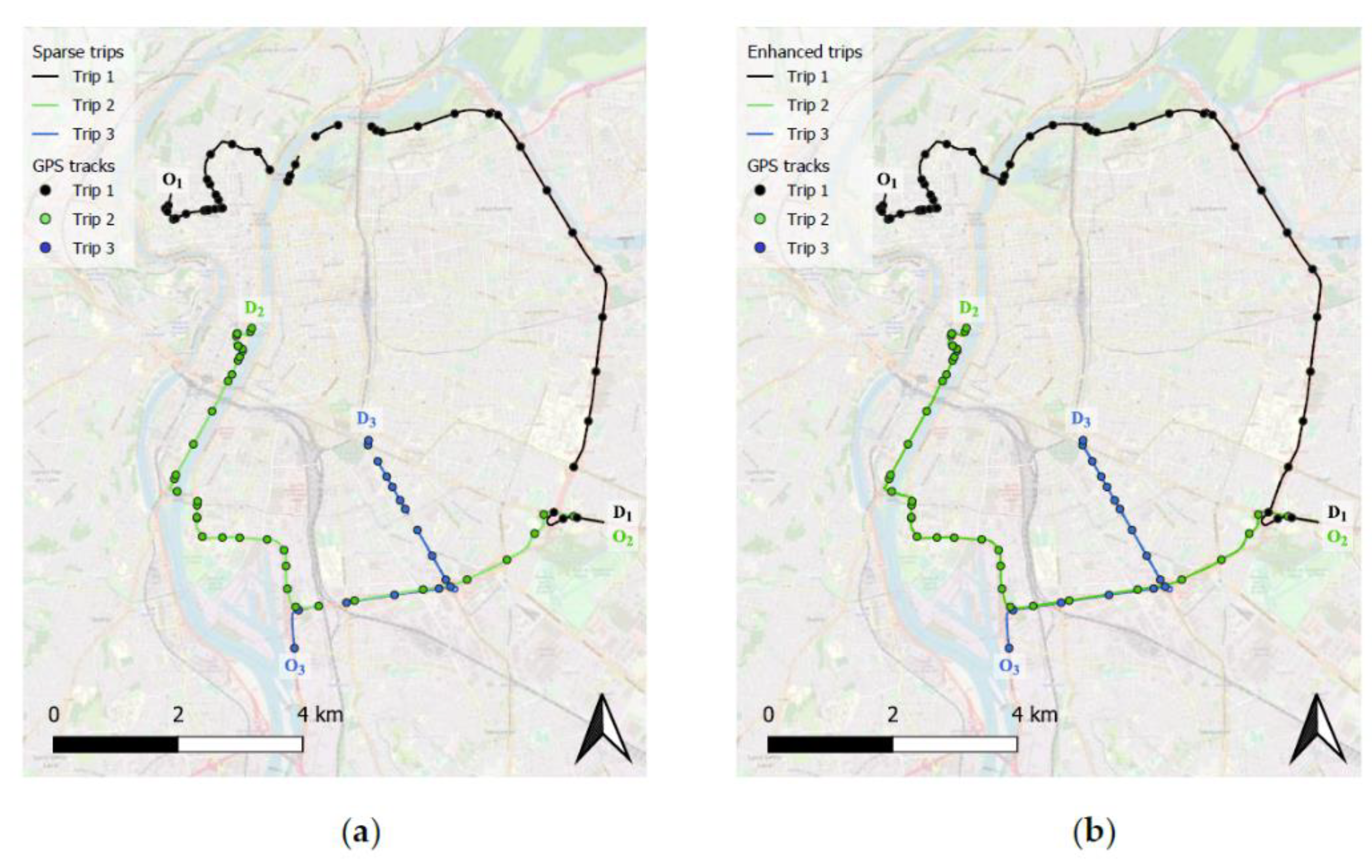
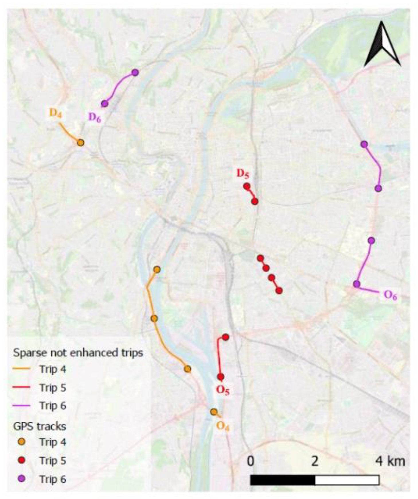
2.2.3. Trip Dataset Processing

The main idea behind the reconstruction of actual trips is to preserve the original pattern of the day’s traffic by reflecting the routes taken initially as closely as possible. Thus, in contrast to the construction of the matrix of mean speed flow where local roads of minor importance characterized by links category 7 are removed, they are conserved in this part to construct the DiGraph of the road network and reconstruct the timestamp. The actual trips of the first ten days of November are restored.

Trip Enhancement

Observations on each link with the timestamp, coverage, and speed are merged with tracks information to reconnect each vehicle ID with its journey. Then, several preprocessing tasks are performed: trips are set on the geographic site studied, journeys lasting two days are processed only on the first day, and those without any observation are removed. Due to the filtering on the area studied, sparse records, or a pause during the journey, some trips may not be continuous, leading to low spatial resolution. Thus, the continuity of links traveled is examined in terms of the space and time for each journey. The trip enhancement method proposed in this work shares the same idea as the trip enrichment method of Papuiri et al. [54]: finding the SP between two nodes to recover an incomplete trip.

In the current work, trip enhancement is processed with the Dijkstra algorithm on a weighted DiGraph using the Python package NetworkX [55]. The weighted DiGraph no.1 is built with simplified links, including frc 7, i.e., 39,812 links. The length of each link is used as a weight to compute the SP and thus to enhance sparse trips. Finally, a threshold of one thousand meters is set to fill missing observations with an SP. The detailed pseudocode for trip enhancement is shown in Point S3 of Supplementary Materials.

Figure 6 displays three typical cases of the trip enhancement method employed for sparse trips. Figure 6a shows GPS traces and their projection on the network performed by MediaMobile (France) for three trips. These trips have missing observations several times, four times for the black trip (352 m, 402 m, 462 m, and 795 m), three times for the blue trip (277 m, 309 m, 628 m), and two times for the green one (355 m, 454 m). Consequently, these routes are enhanced by an SP as many times as necessary while the SP does not exceed the threshold of one thousand meters, as shown in Figure 6b.

However, some journeys may include long-missing observations, with at least one SP longer than the threshold, such as the orange (1458 m, 5681 m), red (2875 m, 291 m, 1946 m), and purple (1594 m, 8808 m) trips displayed in Figure 7. These typical routes were not investigated because of the significant uncertainty involved in extrapolating the path actually traveled. Moreover, some trips are curtailed to the area studied when made both within and outside. Thus, these routes were also removed from our study because it is impossible to find a path to enhance them within Digraph no. 1.

The number of trips studied increased by 50% on average through the enhancement process. Furthermore, the timestamp reconstruction was implemented to meet two primary requirements: the alternative routes search method and the sparseness of actual journeys. The method of searching for alternative trips is based on the reconstitution of traffic conditions, i.e., on average link speeds either observed or deduced by RF. Therefore, the timestamp reconstruction based on the average link speeds is a better way to assess pollutant emissions for the actual trips. Indeed, in this way, pollutant emissions can be estimated at the same scale for both actual and alternative trips.

Trip Selection

It is noteworthy that some trips may be composed of several ODs (e.g., picking up children at school, making quick purchases, etc.), searching for a long time to find a place to park, taking the wrong direction, or a change in destination, etc. Some trips also start and end at the same location, others are only composed of five links or fewer. However, it often does not make sense to find a more eco-friendly alternative path for these actual trips. Therefore, some trips are ruled out because there is no interest in finding an alternative. Moreover, only trips with a TT longer than five minutes are investigated because there is also a minimum interest in studying an alternative path for short journeys and on the other hand.

Moreover, the detour ratio method based on Euclidean distance ($D{R}_{ED}$) is computed to keep only trips for which a sustainable alternative may be considered. Indeed, a straight line is often used to indicate the traveled distance. The definition of $D{R}_{ED}$ is provided by Equation (2) below:

$$D{R}_{ED} =\frac{T{D}_{actual}}{ED},$$

(2)

where $T{D}_{actual}$ is the TD of the actual trip and $ED$ is the Euclidean distance of the OD of this trip. The empirical cumulative distribution function (ECDF) of the $D{R}_{ED}$ showed the same trend for the ten days studied. Thus, trips with a $D{R}_{ED}$ higher than the 97 percentiles of continuous trips ($D{R}_{ED97}$) are filtered from the database. The values of the 97 percentiles ranged from 2.46 to 5.24 with an average of 3.53 and a standard deviation of 1.01. Using this process, about one thousand actual routes two to five times longer than the ED are removed.

However, the method based on $D{R}_{ED}$ was not enough to clean the database entirely. Thus, a visual control is performed by relying on the detour ratio method based on the shortest distance path ($D{R}_{SP}$) defined in Equation (3) below:

$$D{R}_{SP} =\frac{T{D}_{actual}}{T{D}_{SP}},$$

(3)

where $T{D}_{SP}$ is the TD of the shortest path between the OD of the actual trip considered. Finally, nearly two thousand trips checked visually are removed from the database. At the end of the trip selection process, about twelve thousand trips were preserved in the database for the first ten day of November 2017.

2.2.4. Alternative Trip Search

Pollutants Emission Assessment

The pollutant emissions are assessed by the COPERT model, an emission estimation tool at national, regional, or local scale. Recent studies showed applications at street level [56,57], and some papers recommended working with COPERT for trips longer than 500 m [58,59]. The COPERT method assumes that average emissions over a trip change with the average TS. Hot exhaust emissions are measured on a chassis dynamometer of a test vehicle during a specific driving cycle. Then, they are associated with the mean TS over the cycle. Accordingly, the relationship between emissions and average speed is established in emission factors. The COPERT model provides hot exhaust EF for many air pollutants for various vehicle classes (passenger cars, buses, light commercial vehicles, etc.). This study focuses on FC and CO₂, NOx, and PM₁₀ pollutants in passenger cars. The assessment of emission must be carried out on both actual trips and alternative trips. However, our eco-routing method searches the latter by constructing them link by link. Consequently, COPERT is applied at the link level for both types of trips for consistency.

Considering links on the urban network, a trip may be represented by sub-trips for each link traveled. Thus, the emission appraisal relies on local variables for each sub-trip: the mean speed $V_{link}$ (observed or deduced by RF) and the distance $d_{link}$ of the link. Finally, for a pollutant $k$, the total emission $E_{total}^k$ may be assessed by summing the estimated emission on each link as defined in Equation (4):

$$E_{total}^k={\displaystyle \sum }_{link}{d}_{link}\times f^k\left(V_{link}\right),$$

(4)

where $f^k$ is the COPERT emission factor (g/km) of pollutant $k$ aggregated at the fleet level considering the French urban fleet composition. To this end, except link category 7, pollutant emissions are estimated for every link in the network for each interval of fifteen minutes, i.e., 96 intervals.

Furthermore, a multi-pollutants criterion is defined considering the EFs of the three pollutants. The EFs are scaled using their absolute maximum value according to the following Equation (5):

$$f_{scaled}^k =\frac{f^k}{max\left(\left|f^k\right|\right)},$$

(5)

where $f_{scaled}^k$ is the COPERT scaled emission factor (g/km) of pollutant $k$. Finally, the EF of multi-pollutants is computed by weighting the EFs of the three pollutants, as presented in Equation (6):

$$f^{multi-pollutant} =\frac{f_{scaled}^{C{O}_2}}{2}+\frac{f_{scaled}^{NOx}}{4}+\frac{f_{scaled}^{P{M}_{10}}}{4},$$

(6)

Eco-Routing Method

As presented in Section 1.2, several studies have used the Dijkstra algorithm in the eco-routing method. Here, time-dependent eco-routing methods have also been implemented with the Dijkstra algorithm to find alternative paths for our trip dataset. This algorithm is applied on a new weighted DiGraph no. 2. This DiGraph no. 2 is built similarly to DiGraph no. 1. However, DiGraph no. 2 did not contain links frc 7, i.e., 22,796 links are conserved. The link emissions and the link TT are provided on its edges for each time interval. The weighted Dijkstra algorithm provided by NetworkX is used as a basis to investigate alternative eco-friendly paths according to EFs. The time-dependent eco-routing method has relied on a new and improved time-based algorithm. The input data are the DiGraph n 2, the origin, the destination, and the timestamp of the departure. The cumulative TT is also stored by the algorithm along with the cumulative emissions. The emissions costs are updated in real-time according to the time interval when the links were crossed. The SP with link length as cost and the time-dependent FP with link TT are computed to compare the eco-routing method.

3. Results

3.1. Descriptive Analysis

3.1.1. Actual Trips

The actual trips dataset includes 11,497 trips, derived from the GPS dataset, as described previously. The mean TD was 8.33 km, ranging from 0.68 km to 26.50 km. The mean TT was 11.78 min, ranging from 5.00 min to 46.91 min. The mean TS was on average 51.14 km/h, ranging from 6.00 km/h to 86.73 km/h. The travel emission (TE) is provided for each pollutant with more detailed statistics in

Table 2. Descriptive analysis of actual trips.

Statistics	TD (km)	TT (min)	TS (km/h)	TE CO2 (kg)	TE FC (litres)	TE NOx (g)	TE PM10 (g)	TE Multi (No Unit)
Mean	8.33	11.78	51.14	1.44	0.20	4.27	0.09	4.60 × 10−3
Standard deviation	3.68	5.68	17.85	0.58	0.08	1.74	0.04	1.87 × 10−3
Minimum	0.68	5.00	6.00	0.21	0.03	0.56	0.01	0.63 × 10−3
25th percentile	5.52	7.60	35.31	1.00	0.14	2.94	0.06	3.18 × 10−3
50th percentile	7.84	10.31	51.34	1.38	0.19	4.05	0.09	4.38 × 10−3
75th percentile	11.96	14.51	68.21	1.88	0.26	5.66	0.12	6.09 × 10−3
Maximum	26.50	46.91	86.73	4.20	0.57	12.39	0.26	13.36 × 10−3

below:

These trips are distributed over 119 of the 121 possible ODs and over all periods of the day. The most represented origin is region 10 (urban motorway), which corresponds to trips starting outside the urban motorway.

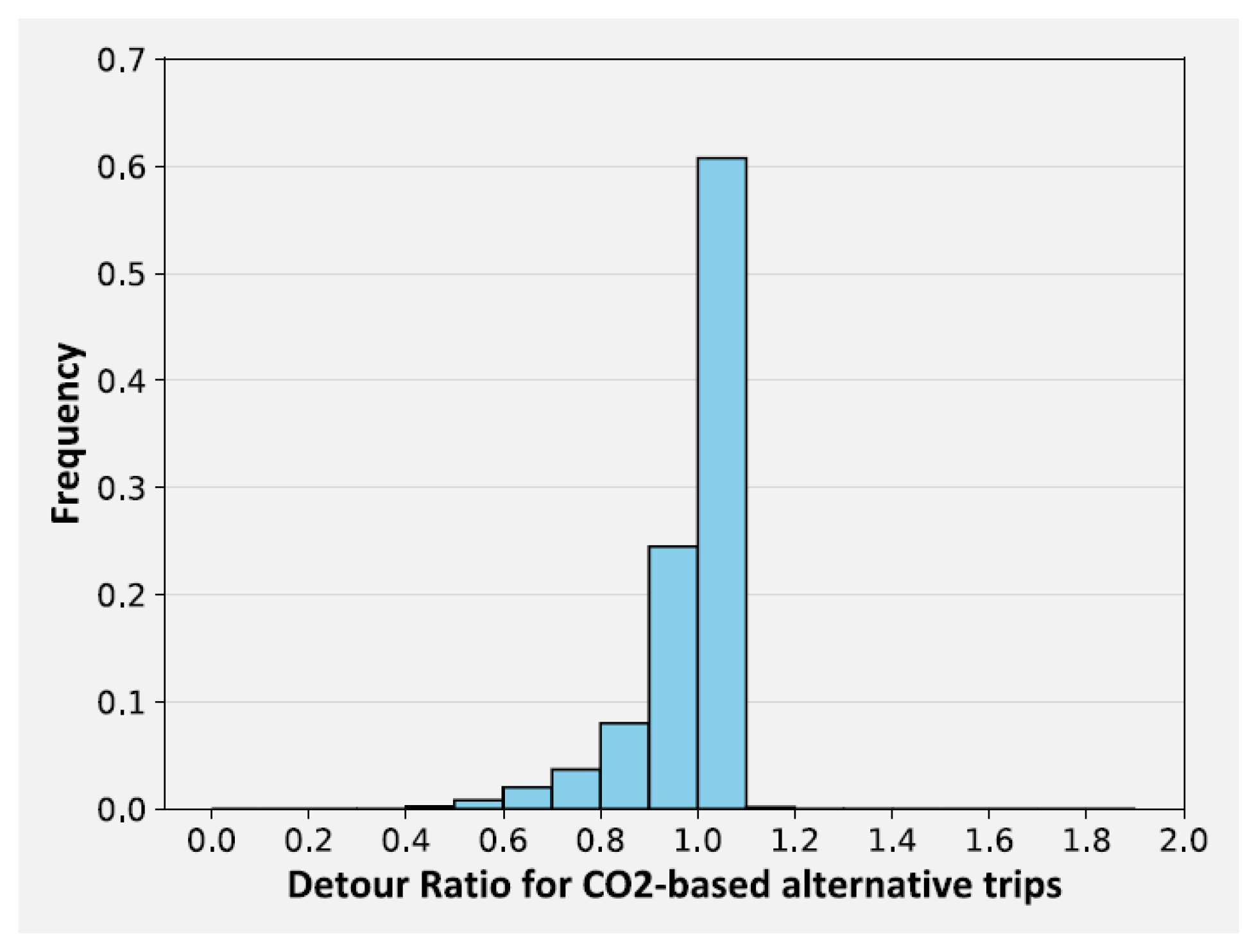
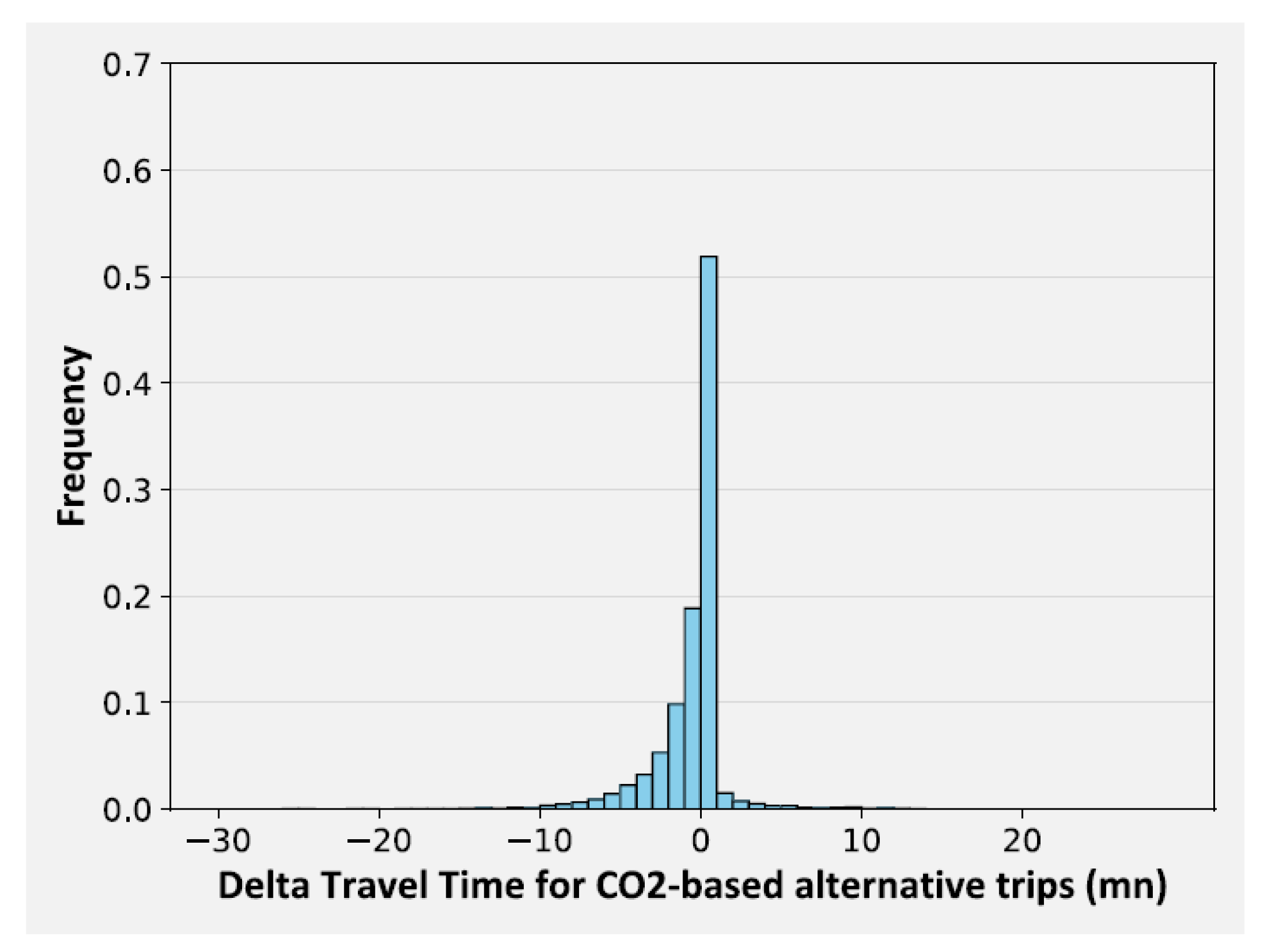
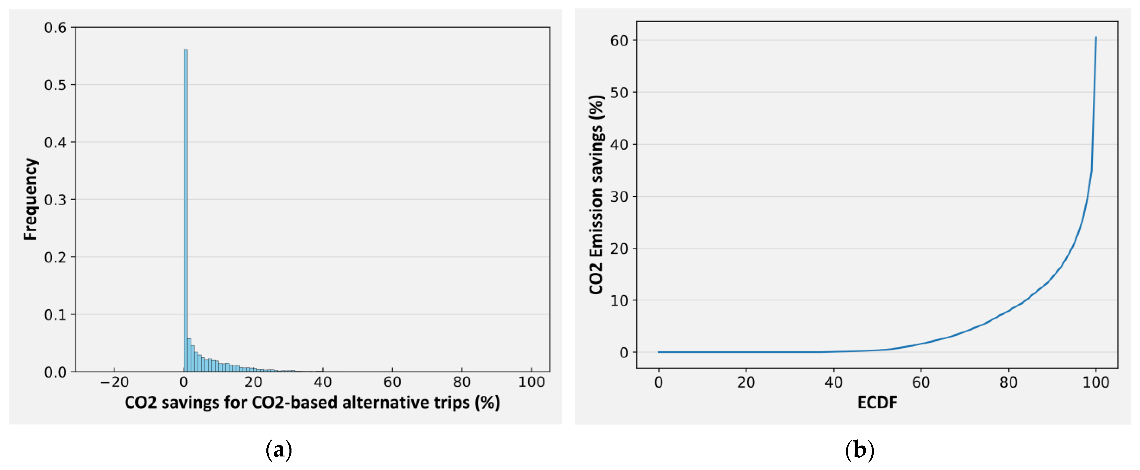
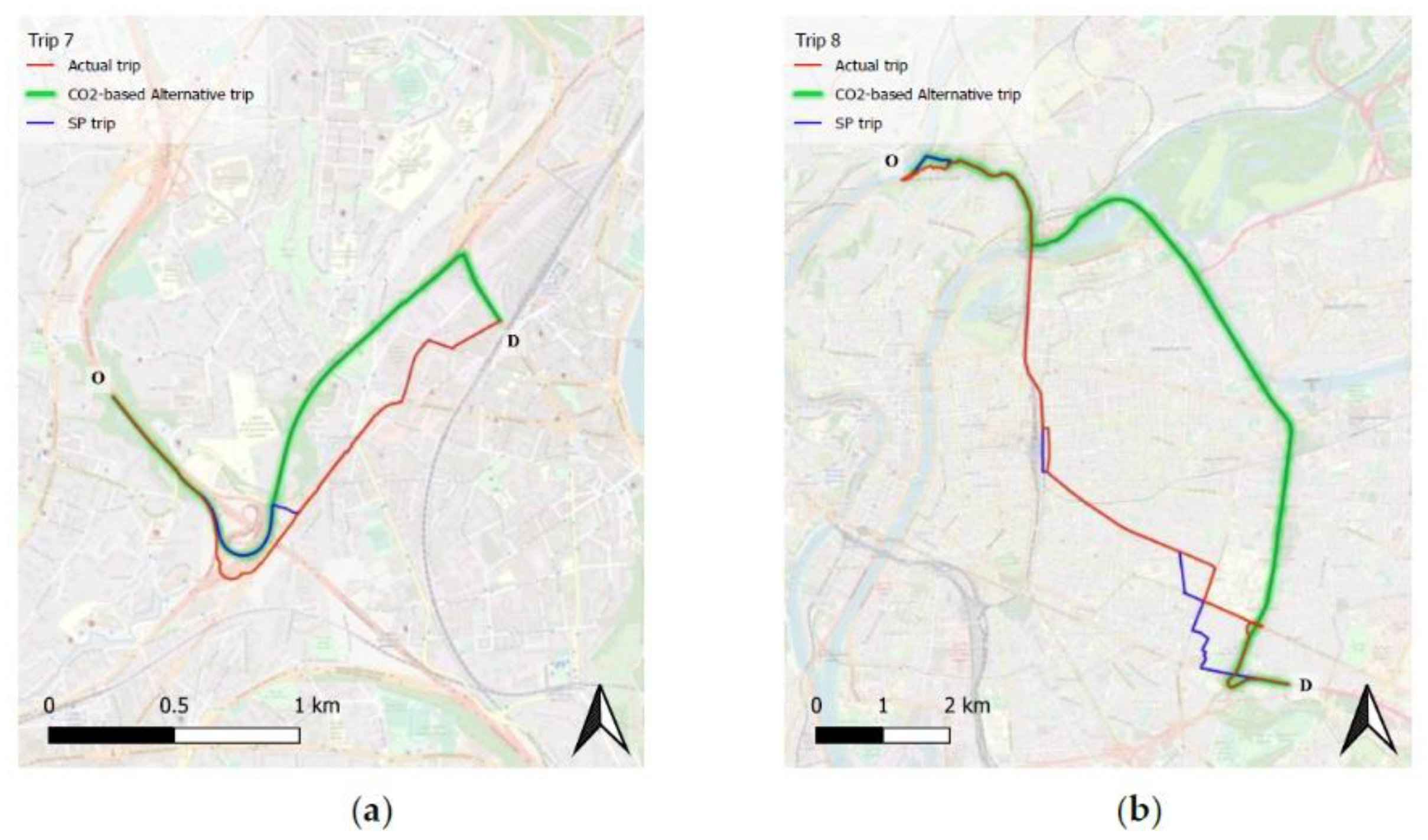
3.1.2. CO₂-Based Alternative Trips

For each actual trip, a CO₂-based alternative trip has been performed, as described in Section 2.2.4. Here the CO₂ emission factor represents a typical vehicle in Lyon, including the fleet composition. The mean TD of CO₂-based alternative trips was 7.99 km which was slightly lower than the actual trips, ranging from 0.68 km to 18,55 km. Similarly, the mean TT was somewhat lower at 11.09 min, ranging from 5.03 min to 43.94 min. Likewise, the mean TS was on average 50.41 km/h ranging from 6.00 km/h to 86.13 km/h. Furthermore, two indicators were computed for each trip to assess the consequences of the alternative path.

First, the detour ratio method induced by sustainable path ($D{R}_{SuP}$) was set to assess the difference in length. The definition of $D{R}_{SuP}$ is provided by Equation (7) below:

$$D{R}_{SuP} =\frac{T{D}_{alternative}}{T{D}_{actual}},$$

(7)

where $T{D}_{alternative}$ is the TD of the alternative trip. The mean $D{R}_{SuP}$ is 0.96, meaning that alternative trips are on average slightly shorter than actual trips, ranging from 0.37 to 1.35. However, as shown in Figure 8, more than half of the CO₂-based alternative trips were between 0% and 10% longer than the actual trips, including 37% traveling the same distance. The $D{R}_{SuP}$ distribution for alternative trips based on other pollutants followed the same trend and are displayed in Point S4 of Supplementary Materials.

Second, the delta travel times ($\Delta TT$) were calculated to assess the time difference. The definition of $\Delta TT$ is provided by Equation (8) below:

$$\Delta TT =T{T}_{alternative}-T{T}_{actual},$$

(8)

where $T{T}_{alternative}$ is the TT of the alternative trip and $T{T}_{actual}$ is the TT of the actual trip. The mean $\Delta TT$ is −0.69 min meaning that alternative trips are on average somewhat faster than actual trips, ranging from −25.73 min to 13.40 min. However, Figure 9 shows that more than half of the CO₂-based alternative trips were between 0 min and 1 min slower than actual trips, including 37% made with the same TT. The $\Delta TT$ distributions of the other pollutants followed the same trend and are displayed in Point S4 of Supplementary Materials. A descriptive analysis of CO₂ alternative trips is provided in

Table 3. Descriptive analysis of CO₂ alternative trips.

Statistics	TD (km)	TT (min)	TS (km/h)	TE CO2 (kg)	DRSuP (No Unit)	∆TT (min)
Mean	7.99	11.09	50.41	1.37	0.96	−0.69
Standard deviation	3.55	5.03	17.66	0.55	0.09	2.24
Minimum	0.68	2.46	6	0.20	0.37	−25.73
25th percentile	5.15	7.26	34.47	0.95	0.97	−1.00
50th percentile	7.63	10.02	50.43	1.30	1	0
75th percentile	11.22	13.47	67.65	1.87	1	0
Maximum	18.55	43.94	86.13	3.19	1.35	13.40

below. The statistics for all the other pollutants are provided in Point S4 of Supplementary Materials. The trend in these statistics is similar for every pollutant, except for the TE.

3.1.3. Shortest Path and Fastest Path

This study also examined the SP and the FP to further assess the impact of eco-routing on TD and TT. The mean TD was 7.88 km for the SP, ranging from 0.68 km to 16.57 km. The mean TT is 13.02 min, ranging from 2,36 min to 53.92 min. The mean TS is on average 44.76 km/h, ranging from 6.00 km/h to 86.13 km/h. The TE is provided for each pollutant with more detailed statistics in

Table 4. Summary statistics of SP alternative trips.

Statistics	TD (km)	TT (min)	TS (km/h)	TE CO2 (kg)	TE FC (litres)	TE NOx (g)	TE PM10 (g)	TE Multi (No Unit)
Mean	7.88	13.02	44.76	1.42	0.19	4.16	0.09	4.50 × 10−3
Standard deviation	3.48	6.64	16.08	0.59	0.08	1.74	0.04	1.88 × 10−3
Minimum	0.68	2.36	6	0.20	0.03	0.56	0.01	0.63 × 10−3
25th percentile	5.08	7.73	31.29	0.97	0.13	2.82	0.06	3.05 × 10−3
50th percentile	7.59	11.88	42.52	1.33	0.18	3.93	0.08	4.24 × 10−3
75th percentile	11.03	16.19	56.93	1.92	0.26	5.73	0.12	6.16 × 10−3
Maximum	16.57	53.92	86.13	3.58	0.49	10.09	0.21	11.1 × 10−3

below:

The mean TD is 8.42 km for the FP, ranging from 0.68 km to 28.10 km. The mean TT is 10.53 min, ranging from 2.36 min to 35.52 min. The mean TS was on average 53.00 km/h, ranging from 9.41 km/h to 86.73 km/h. The TE is provided for each pollutant with more detailed statistics in

Table 5. Summary statistics of FP alternative trips.

Statistics	TD (km)	TT (min)	TS (km/h)	TE CO2 (kg)	TE FC (litres)	TE NOx (g)	TE PM10 (g)	TE Multi (No Unit)
Mean	8.42	10.53	53.00	1.42	0.19	4.21	0.09	4.54 × 10−3
Standard deviation	3.81	4.36	16.82	0.59	0.08	1.77	0.04	1.90 × 10−3
Minimum	0.68	2.36	9.41	0.20	0.03	0.56	0.01	0.63 × 10−3
25th percentile	5.49	7.08	38.65	0.97	0.13	2.87	0.06	3.09 × 10−3
50th percentile	7.86	9.84	53.28	1.34	0.18	3.96	0.08	4.27 × 10−3
75th percentile	11.96	12.87	68.86	1.88	0.26	5.65	0.12	6.07 × 10−3
Maximum	28.10	35.52	86.73	4.48	0.61	13.28	0.29	14.27 × 10−3

below:

As expected, TD was on average the shortest for SP alternative trips and TT was on average the fastest for FP alternative trips compared to other alternative trips. Furthermore, SP and FP alternative trips achieved on average the same TE of FC for FC-based alternative trips and the same TE of PM₁₀ for PM₁₀-based alternative trips. However, they emitted more CO₂, NOx, and multi-pollutants on average.

3.2. Global Analysis: Mean CO₂ Emission Factor

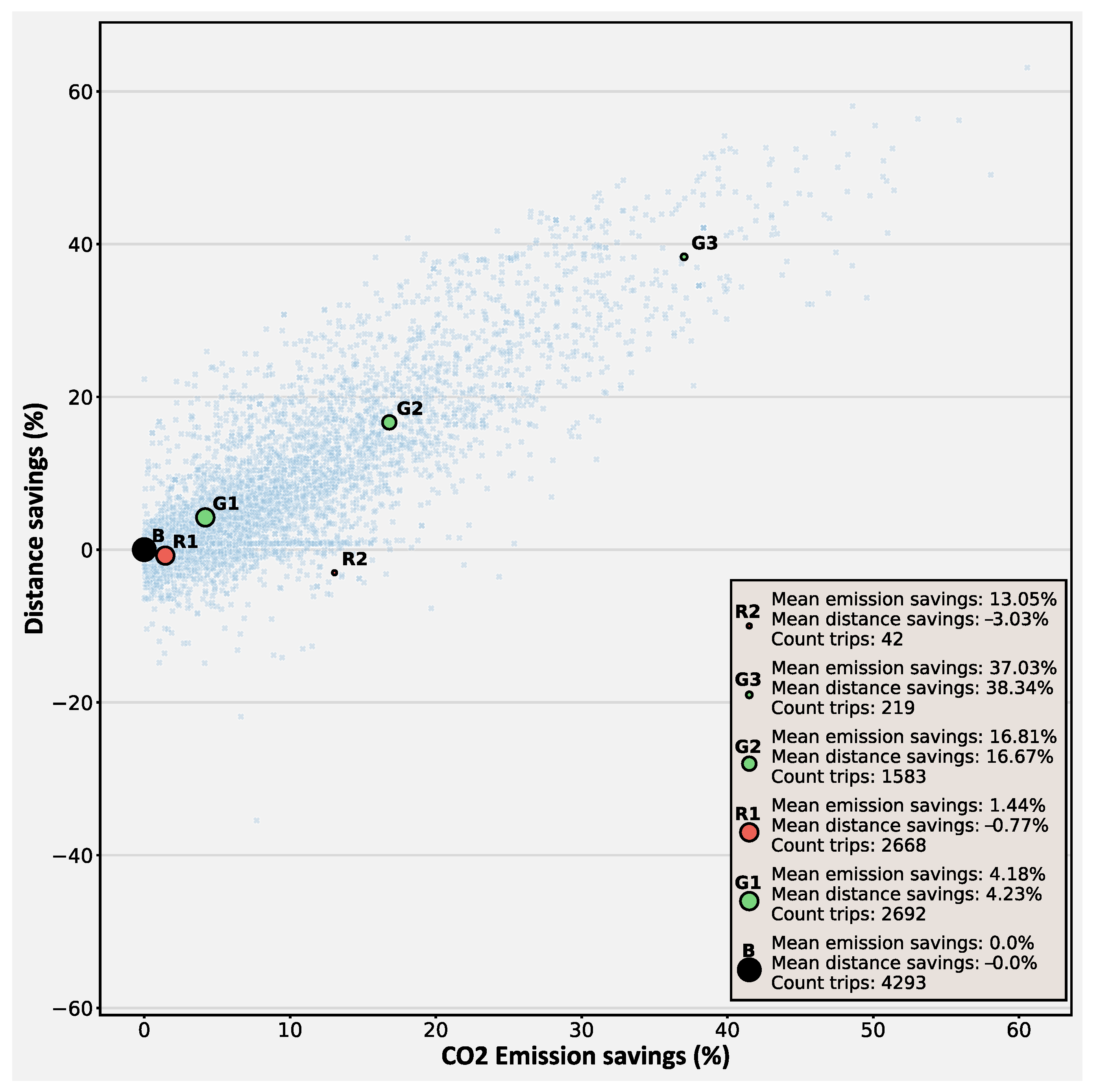
3.2.1. Assessment of CO₂ Emission Savings

The delta travel emission ($\Delta TE$) were computed to assess the emission savings with alternative trips. The definition of $\Delta TE$ is provided by Equation (9) below:

$$\Delta TE=\frac{T{E}_{actual}-T{E}_{alternative}}{T{E}_{actual}}\times 100,$$

(9)

The CO₂ emissions savings were on average 4.38% with a standard deviation of 7.65%. According to our study, there were 7202 trips (63%) with emission savings in the dataset. Thus, there were 4 295 alternative trips (37%) with no emission gains for this pollutant. Apart from a few journeys, they also presented a $\Delta TT=0$ and an $D{R}_{SuP}=1$. This means that the corresponding actual trips in the database had already taken the best eco-friendly path in terms of CO₂ emission, in accordance with our eco-routing method. The CO₂ emissions savings varied from 0% to 60.57%, while about 27% of alternative trips achieved a significant gain higher than 5%. The distribution and the ECDF of CO₂ emissions savings are displayed in Figure 10a,b. Figure 10b shows that almost 20% of trips could have saved at least 10% of CO₂ emission. The gains were of the same order of magnitude regardless of the pollutants considered, and their distribution is provided in Point S5 of Supplementary Materials. The number of trips with emission savings ranges from 63% to 72% depending on the pollutant to be maximized.

Figure 11 shows the repartition of trips according to the CO₂ emission savings and the distance savings. The definition of distance savings is provided by Equation (10) below:

$$\Delta TD=\frac{T{D}_{actual}-T{D}_{alternative}}{T{D}_{actual}}\times 100,$$

(10)

The blue crosses depict each trip ${\tau }_i\left(\Delta T{E}_i,\Delta T{D}_i\right)$ while the dots are the average by region. The black dots correspond to the average of trips with $\Delta TE=0$ and $\Delta TD\approx 0$. The green dot G1, G2 and G3 are defined in Equations (11)–(13):

$$\forall {\tau }_i\left(\Delta T{E}_i,\Delta T{D}_i\right)\in \left[0,10\right[\times {ℝ}_{+}^{*}, \mathrm{G}1=\left(\frac{1}{n}{{\displaystyle \sum }}_i^n\Delta T{E}_i,\frac{1}{n}{{\displaystyle \sum }}_i^n\Delta T{D}_i\right)$$

(11)

$$\forall {\tau }_i\left(\Delta T{E}_i,\Delta T{D}_i\right)\in \left[10,30\right[\times {ℝ}_{+}^{*}, \mathrm{G}2=\left(\frac{1}{n}{{\displaystyle \sum }}_i^n\Delta T{E}_i,\frac{1}{n}{{\displaystyle \sum }}_i^n\Delta T{D}_i\right)$$

(12)

$$\forall {\tau }_i\left(\Delta T{E}_i,\Delta T{D}_i\right)\in \left[30,\infty \right[\times {ℝ}_{+}^{*}, \mathrm{G}3=\left(\frac{1}{n}{{\displaystyle \sum }}_i^n\Delta T{E}_i,\frac{1}{n}{{\displaystyle \sum }}_i^n\Delta T{D}_i\right)$$

(13)

Similarly, the red dot R1 and R2 are defined in Equations (14) and (15):

$$\forall {\tau }_i\left(\Delta T{E}_i,\Delta T{D}_i\right)\in \left[0,10\right[\times {ℝ}_{-}\setminus \left\{0,0\right\}, \mathrm{R}1=\left(\frac{1}{n}{{\displaystyle \sum }}_i^n\Delta T{E}_i,\frac{1}{n}{{\displaystyle \sum }}_i^n\Delta T{D}_i\right)$$

(14)

$$\forall {\tau }_i\left(\Delta T{E}_i,\Delta T{D}_i\right)\in \left[10,\infty \right[\times {ℝ}_{-}, \mathrm{R}2=\left(\frac{1}{n}{{\displaystyle \sum }}_i^n\Delta T{E}_i,\frac{1}{n}{{\displaystyle \sum }}_i^n\Delta T{D}_i\right)$$

(15)

The actual trips may be grouped into three categories according to our eco-routing method, as follows:

• A total of 4293 trips that do not have a more sustainable alternative regardless the TD, i.e., the black dot;
• A total of 4494 trips that have simultaneously a shorter and more sustainable alternative, i.e., the green dots;
• A total of 2710 trips that have both a longer and more sustainable alternative, i.e., the red dots.

The trips that minimize CO₂ emissions are distributed across 99 of 121 ODs and all periods of the day. Looking at the 15 most represented ODs, it is noteworthy that they contain 70% of the sustainable paths, whereas they contain only 44% of trips in the initial database. Thus, there is now a short list of ODs on which trip modifications can provide the most significant benefits. These trips should be prioritized for eco-routing in order to maximize savings. Considering 70% of these sustainable paths, some of them were transit flows (5%) as their trip started and ended on the urban motorway, half were inward flows and 18% were internal flows. Actual trips saving emission pollutants mainly traveled in regions 2, 0, and 3.

It is also quite interesting to note that alternative trips with $\Delta TE>30\%$ all reduce their TD. Furthermore, some alternative trips are longer than the actual trips. Those are the red dots and represent slightly less than a quarter of CO₂ alternative trips. Indeed, as shown in [31,32,33] and confirmed by this study, the SP may not always save the most pollutant emissions. Considering trips with CO₂ emission gains only, these trips are of various lengths. Two interesting alternative routes are displayed in Figure 12 below, first (a) with a short TD of about 3 km, and second (b) with a long TD of about 14 km. Their CO₂ emission savings are higher than 10%, (a) about 20%, and (b) 15%, respectively, with a $D{R}_{EP}$ higher than 1. An alternative path was found for these trips with significant emission savings while their TD increased compared to the actual one.

Regarding the SP, on average the CO₂-based alternative trips slightly increased the TD by about 1.31%. Furthermore, they had a longer TT on average than the FP by about 4.38%. However, they emitted less CO₂ than these trips, about 2.50% less for FP and 2.41% for SP.

3.2.2. Assessment of Other Pollutants

By optimizing CO₂, there are 7202 trips (63%) with CO₂ emission savings. On the basis of these routes, 6894 also presented gains for FC and for other pollutants (NOx, PM₁₀), meaning that the majority of alternative trips (96%) with CO₂ emission gains may also have saved FC and other pollutants at the same time. Then, CO₂-based alternative trips with CO₂ emission savings were compared to alternative trips optimizing other pollutants. About 40% of alternative trips took the same eco-friendly path according to our eco-routing method, regardless of the pollutant considered. Thus, alternative trips to reduce FC, CO₂, NOx, PM₁₀ or multi-pollutant emissions also resulted in optimized benefits for all of them simultaneously. The distribution of gains induced by CO₂ alternative trips is shown in Figure 13 below, according to four criteria (no gains, gains for CO₂ emission only, gains for all pollutants in optimizing CO₂, and optimized gains for all pollutants regardless of the optimized pollutant).

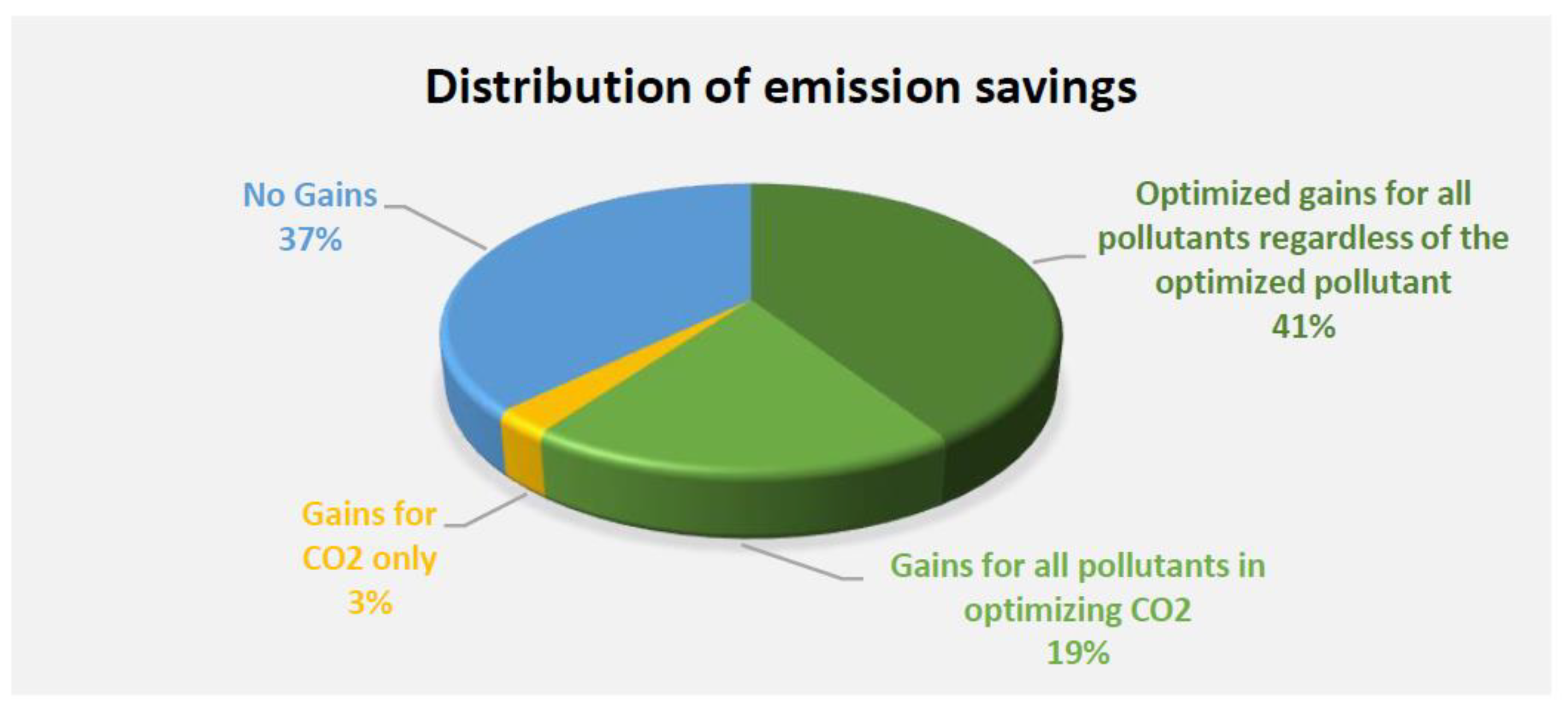
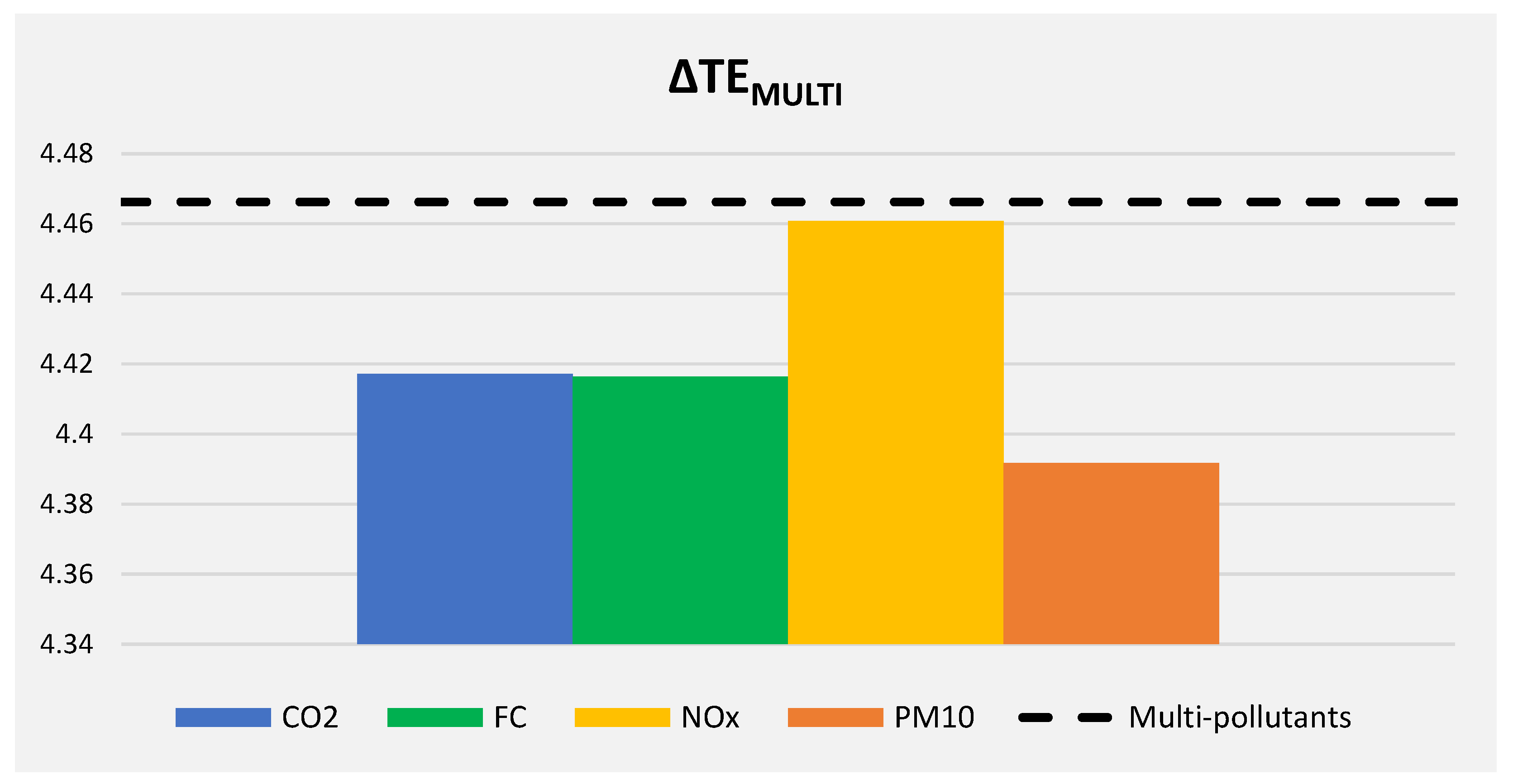
3.2.3. Assessment of Multi-Pollutant Criterion

By optimizing PM₁₀, more alternative trips were found with emissions savings of over 5% and 20%. Similarly, more alternative trips were found with emissions savings higher than 10% by optimizing FC.

Table 6. Alternative trips found by emission saving category and pollutant optimized.

Pollutant	Trips for ∆TE > 5%	Trips for ∆TE > 10%	Trips for ∆TE > 20%
CO2	3089 (27%)	1844 (16%)	636 (5%)
FC	3090 (27%)	18461 (16%)	635 (5%)
NOx	3006 (26%)	1774 (15%)	650 (6%)
PM10	31501 (27%)	1818 (16%)	6821 (6%)
Multi-pollutants	3067 (27%)	1820 (16%)	647 (6%)

¹ Maximum amount of alternative path according to the emission saving category.

provides the number of alternative trips found according to the emission saving category and pollutant optimized. The multi-pollutant criterion increased the minimum number of alternative trips found for each emission saving category (5%, 10%, and 20%).

The multi-pollutant criterion is a good compromise regardless of the pollutant optimized. The emission savings based on this criterion are still, on average, very close to those of the optimized pollutant and more significant than those of the other non-optimized pollutants. By optimizing NOx, the emission gains are close on average to those optimized by the multi-pollutant criterion but a bit lower. The representation of average emission savings per trip is provided for each pollutant studied in Point S6 of Supplementary Materials. Moreover, multi-pollutant emission savings from NOx-based alternative trips are very close on average to those from multi-pollutant-based alternative trips, as shown in Figure 14.

Although alternative trips based on the multi-pollutant criterion come close to the TE of the alternative trips based on the pollutant of interest, they led to a somewhat higher TD or TT cost compared to the SP and the FP, respectively. Indeed, regarding the SP, on average the CO₂-based alternative trips slightly increased the TD by about 1.28%. Furthermore, they had a longer TT on average than the FP by about 5.62%.

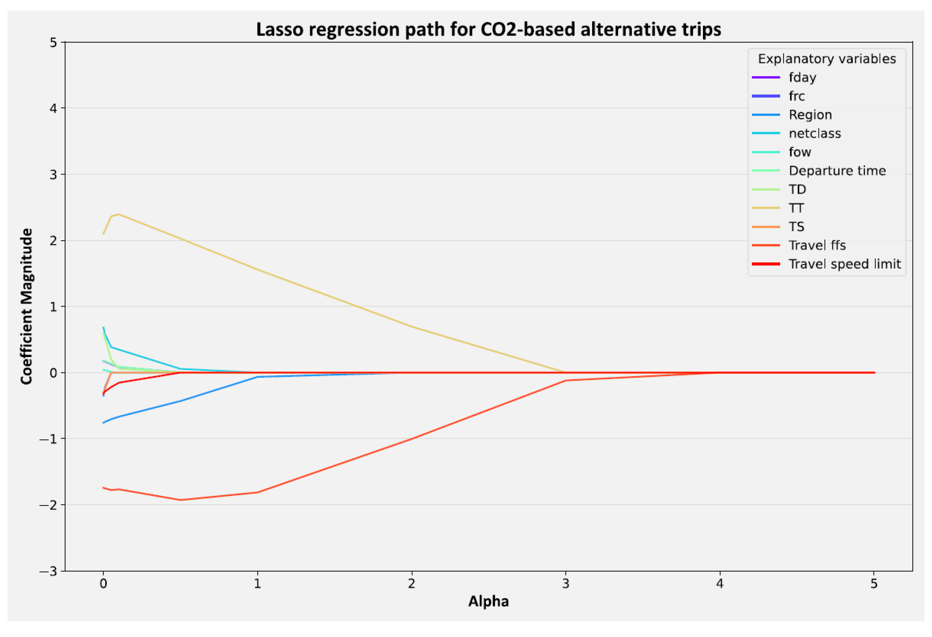
3.2.4. Explanatory Variables

The LASSO regression method [60] was computed in an attempt to identify variables that may explain the emission savings. These explanatory variables could be useful in targeting a subset of trips that offer the best gains. To this end, eleven variables were defined, including fday, frc, netclass, fow, region, departure time, TD, TT, TS, travel ffs, and travel speed limit. These features were chosen due to their potential capability to explain gains. Since frc, netclass, fow, and region are categorical variables that depend on the link traversed, the value with the highest frequency was chosen as input. Travel ffs and the travel speed limit were computed similarly to the TS.

Figure 15 presents the LASSO regression results for alternative trips based on CO₂ as a function of the alpha coefficient. Four explanatory features can be seen which could explain emission savings for every pollutant (region, netclass, TT, Travel ffs). The trend is the same regardless of the pollutant optimized by alternative trips. The LASSO regression results for alternative trips are provided for each pollutant in Point S6 of Supplementary Materials. Most of the highest multi-pollutant emission savings were achieved for actual trips using the urban motorway or netclass 2 links (medium importance). These trips had the particularity of being quite long (more than 15 min on average) with a moderate travel ffs (45 km/h on average). Moreover, the LASSO regression highlights regions as one of the four explanatory variables capable of explaining emission savings. This could be justified by the fact that the expected savings are not uniformly distributed in space, which was confirmed in their analysis considering ODs. Consequently, it is noteworthy that trip locations have more impact than their departure time in view to maximize the environmental benefits.

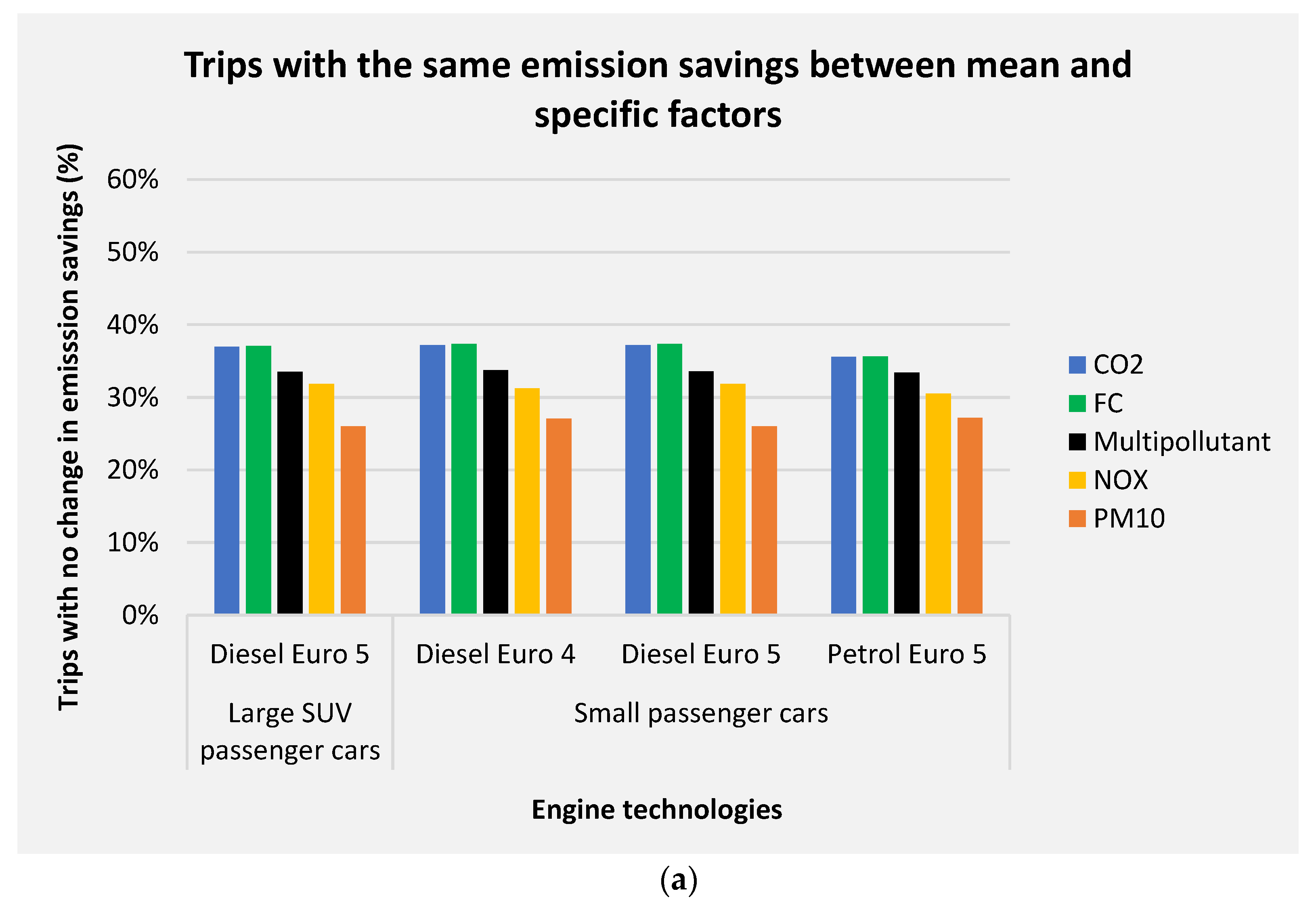
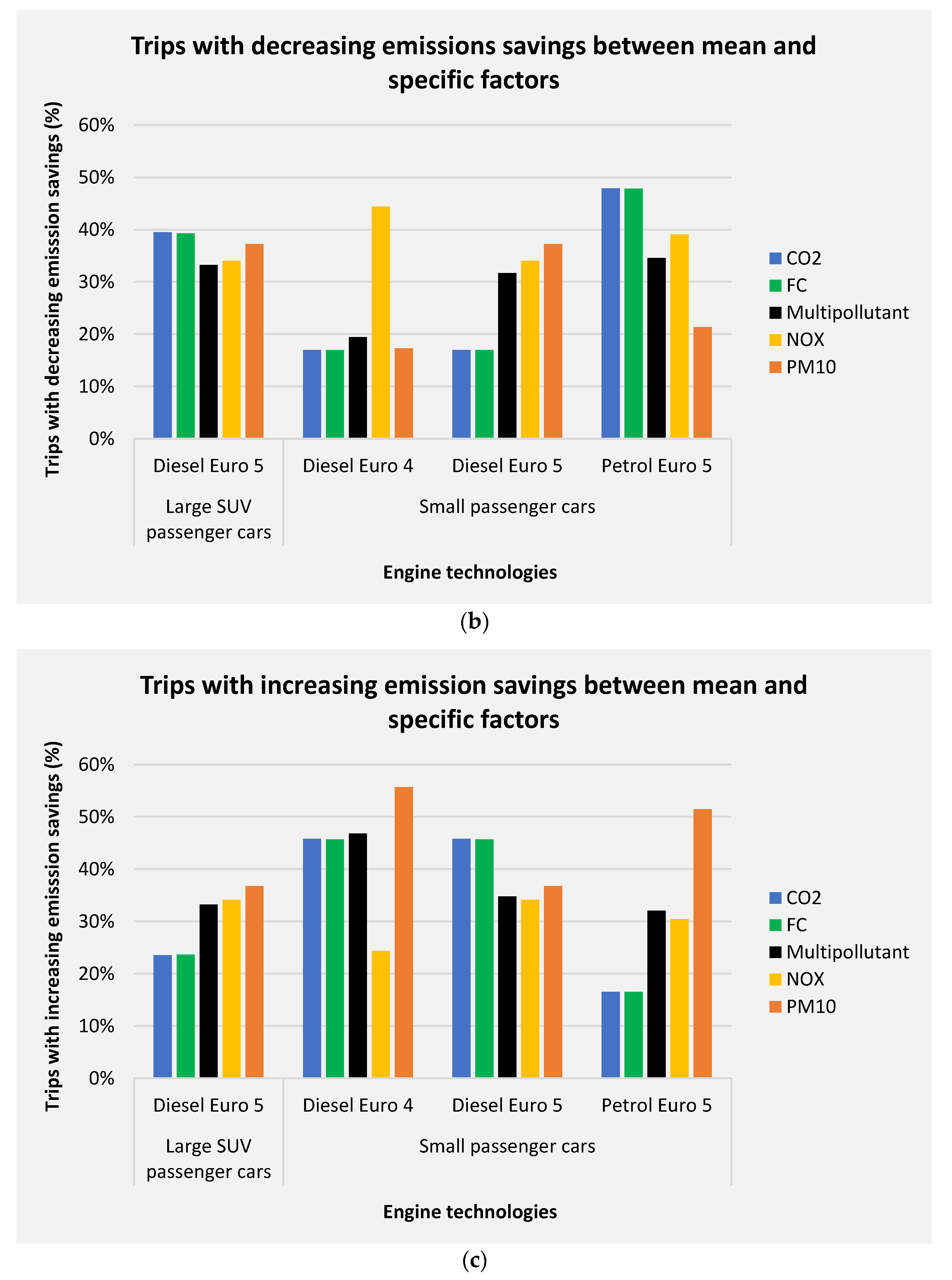
3.3. Investigating the Influence of the Emission Factor

Emission Savings Analysis

In this part, we investigate the influence of the EF according to the type of vehicle (large SUV passenger cars and small passenger cars) and the engine technologies (diesel/petrol euro 4 and euro 5). A total of twenty EFs were studied for all trips in the database. The objective was to compare the results between the EFs for a standard vehicle, such as the mean CO₂ EF, and the EFs for a more specific vehicle.

Overall, fewer alternative trips were found with emission gains for specific EFs than for mean EFs. Indeed, fifteen specific EFs had between 51% and 56% of alternative trips with an $\Delta TE>0$ and five above 63%. Comparatively, mean EFs all had more than 63% of alternative routes with an $\Delta TE>0$.

However, when emissions gains of more than 5% were considered, the number of alternative trips found for the specific EF presented the same trend as the mean EFs, regardless of the engine technology, the type of vehicle, and the pollutant optimized. Indeed, there were, respectively, 25–28%, 15–17%, and 5–6% of alternative trips with emission savings above 5%, 10%, and 20% for all the specific EFs. In comparison, there were, respectively, 26–27%, 15–16%, 5–6% of alternative trips with emission savings above 5%, 10%, and 20% for all the mean EFs.

Figure 16 shows the evolution of emission savings between the mean EFs and the specific ones. Figure 16a presents alternative trips with the same emission savings regardless of the EF. A large share of these trips had an $\Delta TE=0$, including 2874 trips with an $\Delta TE=0$ common to all EFs. That means that 25% of the entire dataset had already taken the EP and our eco-routing method was not capable of finding a better path whatever the EF. Figure 16b shows alternative trips with less efficient emission savings for specific EFs than for mean EFs. That shows the share of alternative trips from mean EFs with an $\Delta TE>0$ saving fewer emissions with the specific EFs. Alternative trips with a positive evolution from the mean EFs to the specific ones are provided in Figure 16c. These are either alternative trips from mean EFs with an $\Delta TE>0$ or $\Delta TE=0$ saving more emissions with the specific EFs.

Finally, it is very interesting to emphasize that 414 trips, or about 4% of the dataset, presented emission savings higher than 20% regardless of the emission factor. While the EP could be longer than the SP, these trips were all shorter than those actually made. Indeed, their $D{R}_{SuP}$ was between 0.36 and 0.99. Moreover, it can also be seen that their distribution was quite similar for all the days studied, with fewer trips on Wednesdays, weekends, bank holidays, and holidays. This last point may be explained by the distribution of trips presented in Figure 2.

4. Discussion

The use of GPS traces requires processing to answer the research questions defined in Section 1.3 above. From the GPS traces, it is necessary to extract variables capable of estimating the emissions of a trip and seek a sustainable path. However, these data are incomplete due to the lack of observations on certain links. Thus, several network links do not have speed information every time. In addition, trip records are sometimes sparse, leading to partial trips which are then a challenge when assessing pollutant emissions of actual trips. Moreover, some trips are not interesting to study an alternative path more eco-friendly for a variety of reasons such as finding a place to park, taking the wrong direction, etc. This work proposes a three-part framework to address these challenges. Firstly, a random forest is trained from the partial data to tackle the missing mean speed flow and thus estimate the network traffic condition every fifteen minutes for the whole month of November 2017. Secondly, actual trips are enhanced using a Dijkstra algorithm and selected on the basis of the detour ratio principle in order to construct a reliable trips dataset. Finally, a DiGraph of the network is constructed with pollutant emissions. These emissions are estimated for each interval of fifteen minutes with a COPERT macroscopic emission model based on the average link speed. A time-dependent Dijkstra algorithm is then applied to this DiGraph to find alternative sustainable paths.

Depending on the pollutant for an average vehicle, there were between 63% and 72% of alternative journeys with emissions savings. These savings ranged up to about 60%, with a quarter of the trips saving at least 5%. Their travel distance (TD) may be short or long with significant or low gains for both. The optimized gains may be obtained by accepting, on average, less than one minute more travel time (TT) than the fastest paths (FPs) and about one hundred meters more than the shortest paths (SPs). While the TD of sustainable paths (SuPs) may be shorter or longer, alternative trips with $\Delta TE>30\%$ all reduce their TD. Moreover, about 40% of alternative trips took the same eco-friendly path and thus simultaneously reached optimized gains for all the pollutants.

This study also highlighted that, on average, the SuPs are slightly shorter and faster than the actual trips, regardless of emissions factors (EFs). Nevertheless, depending on the pollutant for an average vehicle, between 58% and 61% of SuPs have the same TD as or higher than the actual trips. Likewise, between 68% and 81% of SuPs have the same or smaller TT.

The SPs and FPs seem to be a good alternative when the aim is to save PM₁₀ or FC. However, the SPs tend to increase the TT while the FPs increase the TD. Furthermore, neither seem to be a good choice when the aim is to save CO₂ and NOx.

In addition, the multi-pollutant criterion defined in this study seems to be a helpful compromise to optimize all pollutants simultaneously for the mean EFs. The emission savings are always, on average, very close to the optimized gains by using it as an objective. Moreover, this study showed that optimizing NOx may also be a suitable choice to optimize gains for all the pollutants at once.

The LASSO regression method emphasized four explanatory variables explaining emission savings for mean EFs (region, netclass, TT, Travel ffs). Most of the significant multi-pollutant emission savings were obtained when the actual routes used the urban motorway or netclass 2 links. The trips that minimize CO₂ emissions are distributed across 99 of 121 ODs and all periods of the day. Looking at the 15 most represented ODs, it is noteworthy that they contain 70% of the sustainable paths, whereas they contain only 44% of trips in the initial database. Thus, a short list of ODs on which path modifications can provide the most significant benefits is now available in view to prioritize trips for eco-routing and maximize savings.

An analysis of the influence of the EF was performed with twenty specific EFs. It appeared that fewer SuPs were found than for the mean EFs. However, as the emission gains were significant, i.e., more than 5%, the number of SuPs found tended to be the same regardless of the EFs. Finally, this study highlighted 414 trips where more than 20% of pollutant emissions could be saved irrespective of the EFs. Recent measures were recently adopted in France requiring navigation applications to provide environmental information. This study provides insight into the possible gains they could bring in terms of emissions. However, this work was performed for individual trajectories, considering stable traffic conditions. Modifying the original path may have a significant impact on the network, create new traffic states and thus change the optimized path regarding the EFs studied. The mean speed flow thus modified leads to recalculating our results until a collective equilibrium is reached. Consequently, future work will investigate how to manage alternative trips within the network, taking into account the non-linearity of traffic phenomena, using traffic microsimulation.

References

1. International Agency for Research on Cancer (IARC). Air Pollution and Cancer; IARC Scientific: Lyon, France, 2013; ISBN 978-92-832-2166-1.
2. International Agency for Research on Cancer (IARC). IARC Monographs on the Evaluation of Carcinogenic Risks to Humans. In Outdoor Air Pollution; IARC: Lyon, France, 2015; ISBN 978-92-832-0175-5. [Google Scholar]
3. Van Zelm, R.; Preiss, P.; van Goethem, T.; Dingenen, R.V.; Huijbregts, M. Regionalized Life Cycle Impact Assessment of Air Pollution on the Global Scale: Damage to Human Health and Vegetation. Atmos. Environ. 2016, 134, 129–137. [Google Scholar] [CrossRef] [Green Version]
4. Rai, P.K. Impacts of Particulate Matter Pollution on Plants: Implications for Environmental Biomonitoring. Ecotoxicol. Environ. Saf. 2016, 129, 120–136. [Google Scholar] [CrossRef] [PubMed]
5. Popek, R.; Przybysz, A.; Gawrońska, H.; Klamkowski, K.; Gawroński, S.W. Impact of Particulate Matter Accumulation on the Photosynthetic Apparatus of Roadside Woody Plants Growing in the Urban Conditions. Ecotoxicol. Environ. Saf. 2018, 163, 56–62. [Google Scholar] [CrossRef] [PubMed]
6. Pachauri, R.K.; Allen, M.R.; Barros, V.R.; Broome, J.; Cramer, W.; Christ, R.; Church, J.A.; Clarke, L.; Dahe, Q.; Dasgupta, P.; et al. Climate Change 2014: Synthesis Report; Intergovernmental Panel on Climate Change: Geneva, Switzerland, 2015; ISBN 978-92-9169-143-2. [Google Scholar]
7. Monks, P.S.; Archibald, A.T.; Colette, A.; Cooper, O.; Coyle, M.; Derwent, R.; Fowler, D.; Granier, C.; Law, K.S.; Mills, G.E.; et al. Tropospheric Ozone and Its Precursors from the Urban to the Global Scale from Air Quality to Short-Lived Climate Forcer. Atmos. Chem. Phys. 2015, 15, 8889–8973. [Google Scholar] [CrossRef] [Green Version]
8. World Health Organization. Compendium of WHO and Other UN Guidance on Health and Environment; World Health Organization: Geneva, Switzerland, 2021. [Google Scholar]
9. Shang, J.; Zheng, Y.; Tong, W.; Chang, E.; Yu, Y. Inferring Gas Consumption and Pollution Emission of Vehicles throughout a City. In Proceedings of the 20th ACM SIGKDD International Conference on Knowledge Discovery and Data Mining, New York, NY, USA, 24–27 August 2014; ACM: New York, NY, USA, 2014; pp. 1027–1036. [Google Scholar]
10. Macedo, E.; Tomás, R.; Fernandes, P.; Coelho, M.C.; Bandeira, J.M. Quantifying Road Traffic Emissions Embedded in a Multi-Objective Traffic Assignment Model. Transp. Res. Procedia 2020, 47, 648–655. [Google Scholar] [CrossRef]
11. Hausberger, S.; Rodler, J.; Sturm, P.; Rexeis, M. Emission Factors for Heavy-Duty Vehicles and Validation by Tunnel Measurements. Atmos. Environ. 2003, 37, 5237–5245. [Google Scholar] [CrossRef]
12. Zallinger, M.S.; Le Anh, T. Improving an Instantaneous Emission Model for Passenger Cars. In Proceedings of the 14th Symposium Transport and Air Pollution; Verlag der Technischen Universität Graz: Graz, Austria, 2005; Volume 85/I, pp. 166–167. [Google Scholar]
13. Barth, M.; An, F.; Younglove, T.; Scora, G.; Levine, C.; Ross, M.; Wenzel, T.P. Development of a Comprehensive Modal Emissions Model. Transp. Res. Rec. J. Transp. Res. Board 2000, 1587, 52–62. [Google Scholar]
14. AVL. Vehicle Driveline Simulation. Available online: https://www.avl.com/cruise (accessed on 2 January 2022).
15. Tu, R.; Kamel, I.; Wang, A.; Abdulhai, B.; Hatzopoulou, M. Development of a Hybrid Modelling Approach for the Generation of an Urban On-Road Transportation Emission Inventory. Transp. Res. Part D Transp. Environ. 2018, 62, 604–618. [Google Scholar] [CrossRef]
16. Lejri, D.; Can, A.; Schiper, N.; Leclercq, L. Accounting for Traffic Speed Dynamics When Calculating COPERT and PHEM Pollutant Emissions at the Urban Scale. Transp. Res. Part D Transp. Environ. 2018, 63, 588–603. [Google Scholar] [CrossRef] [Green Version]
17. Boulter, P.; McCrae, I. ARTEMIS: Assessment and Reliability of Transport Emission Models and Inventory Systems—Final Report. In TRL Published Project Report; TRL: Crowthorne, UK, 2007. [Google Scholar]
18. Hausberger, S.; Rexeis, M.; Zallinger, M.; Luz, R. Emission Factors from the Model PHEM for the HBEFA Version 3; Report Nr. I-20/2009; Institute for Internal Combustion Engines and Thermodynamics, Graz Uniervisty of Technology: Graz, Austria, 2009. [Google Scholar]
19. Ntziachristos, L.; Gkatzoflias, D.; Kouridis, C.; Samaras, Z. COPERT: A European Road Transport Emission Inventory Model. In Proceedings of the Information Technologies in Environmental Engineering; Athanasiadis, I.N., Rizzoli, A.E., Mitkas, P.A., Gómez, J.M., Eds.; Springer: Berlin/Heidelberg, Germany, 2009; pp. 491–504. [Google Scholar]
20. Rodriguez-Rey, D.; Guevara, M.; Linares, M.P.; Casanovas, J.; Salmerón, J.; Soret, A.; Jorba, O.; Tena, C.; García-Pando, C.P. A Coupled Macroscopic Traffic and Pollutant Emission Modelling System for Barcelona. Transp. Res. Part D Transp. Environ. 2021, 92, 102725. [Google Scholar] [CrossRef]
21. Nguyen, M.H.; Armoogum, J.; Madre, J.-L.; Garcia, C. Reviewing Trip Purpose Imputation in GPS-Based Travel Surveys. J. Traffic Transp. Eng. Engl. Ed. 2020, 7, 395–412. [Google Scholar] [CrossRef]
22. Ashbrook, D.; Starner, T. Using GPS to Learn Significant Locations and Predict Movement across Multiple Users. Pers. Ubiquitous Comput. 2003, 7, 275–286. [Google Scholar] [CrossRef]
23. Lin, M.; Hsu, W.-J. Mining GPS Data for Mobility Patterns: A Survey. Pervas. Mob. Comput. 2014, 12, 1–16. [Google Scholar] [CrossRef]
24. D’Andrea, E.; Marcelloni, F. Detection of Traffic Congestion and Incidents from GPS Trace Analysis. Expert Syst. Appl. 2017, 73, 43–56. [Google Scholar] [CrossRef]
25. Erdelić, T.; Carić, T.; Erdelić, M.; Tišljarić, L.; Turković, A.; Jelušić, N. Estimating Congestion Zones and Travel Time Indexes Based on the Floating Car Data. Comput. Environ. Urban Syst. 2021, 87, 101604. [Google Scholar] [CrossRef]
26. Castro, P.S.; Zhang, D.; Li, S. Urban Traffic Modelling and Prediction Using Large Scale Taxi GPS Traces. In Proceedings of the Pervasive Computing; Kay, J., Lukowicz, P., Tokuda, H., Olivier, P., Krüger, A., Eds.; Springer: Berlin/Heidelberg, Germany, 2012; pp. 57–72. [Google Scholar]
27. Seppecher, M.; Leclercq, L.; Furno, A.; Lejri, D.; da Rocha, T.V. Estimation of Urban Zonal Speed Dynamics from User-Activity-Dependent Positioning Data and Regional Paths. Transp. Res. Part C Emerg. Technol. 2021, 129, 103183. [Google Scholar] [CrossRef]
28. Du, J.; Aultman-Hall, L. Increasing the Accuracy of Trip Rate Information from Passive Multi-Day GPS Travel Datasets: Automatic Trip End Identification Issues. Transp. Res. Part A Policy Pract. 2007, 41, 220–232. [Google Scholar] [CrossRef]
29. Zhang, J.; Wang, F.-Y.; Wang, K.; Lin, W.-H.; Xu, X.; Chen, C. Data-Driven Intelligent Transportation Systems: A Survey. IEEE Trans. Intell. Transp. Syst. 2011, 12, 1624–1639. [Google Scholar] [CrossRef]
30. Leclercq, L.; Chiabaut, N.; Trinquier, B. Macroscopic Fundamental Diagrams: A Cross-Comparison of Estimation Methods. Transp. Res. Part B Methodol. 2014, 62, 1–12. [Google Scholar] [CrossRef]
31. Barth, M.; Boriboonsomsin, K.; Vu, A. Environmentally-Friendly Navigation. In Proceedings of the IEEE Conference on Intelligent Transportation Systems, Bellevue, WA, USA, 30 September–3 October 2007; pp. 684–689. [Google Scholar]
32. Ahn, K.; Rakha, H.A. Network-Wide Impacts of Eco-Routing Strategies: A Large-Scale Case Study. Transp. Res. Part D Transp. Environ. 2013, 25, 119–130. [Google Scholar] [CrossRef]
33. Zeng, W.; Miwa, T.; Morikawa, T. Prediction of Vehicle CO2 Emission and Its Application to Eco-Routing Navigation. Transp. Res. Part C Emerg. Technol. 2016, 68, 194–214. [Google Scholar] [CrossRef]
34. Sun, J.; Liu, H.X. Stochastic Eco-Routing in a Signalized Traffic Network. Transp. Res. Part C Emerg. Technol. 2015, 59, 32–47. [Google Scholar] [CrossRef]
35. Wang, J.; Elbery, A.; Rakha, H.A. A Real-Time Vehicle-Specific Eco-Routing Model for On-Board Navigation Applications Capturing Transient Vehicle Behavior. Transp. Res. Part C Emerg. Technol. 2019, 104, 1–21. [Google Scholar] [CrossRef]
36. Ericsson, E.; Larsson, H.; Brundell-Freij, K. Optimizing Route Choice for Lowest Fuel Consumption—Potential Effects of a New Driver Support Tool. Transp. Res. Part C Emerg. Technol. 2006, 14, 369–383. [Google Scholar] [CrossRef]
37. Gazis, A.; Fontes, T.; Bandeira, J.; Pereira, S.; Coelho, M.C. Integrated Computational Methods for Traffic Emissions Route Assessment. In Proceedings of the 5th ACM SIGSPATIAL International Workshop on Computational Transportation Science—IWCTS ’12, Redondo Beach, CA, USA, 6 November 2012; ACM Press: Redondo Beach, CA, USA, 2012; pp. 8–13. [Google Scholar]
38. Yao, E.; Song, Y. Study on Eco-Route Planning Algorithm and Environmental Impact Assessment. J. Intell. Transp. Syst. 2013, 17, 42–53. [Google Scholar] [CrossRef]
39. Zeng, W.; Miwa, T.; Morikawa, T. Application of the Support Vector Machine and Heuristic K-Shortest Path Algorithm to Determine the Most Eco-Friendly Path with a Travel Time Constraint. Transp. Res. Part D Transp. Environ. 2017, 57, 458–473. [Google Scholar] [CrossRef]
40. Zeng, W.; Miwa, T.; Morikawa, T. Eco-Routing Problem Considering Fuel Consumption and Probabilistic Travel Time Budget. Transp. Res. Part D Transp. Environ. 2020, 78, 102219. [Google Scholar] [CrossRef]
41. Sugawara, S.; Niemeier, D.A. How Much Can Vehicle Emissions Be Reduced? Exploratory Analysis of an Upper Boundary Using an Emissions-Optimized Trip Assignment. Transp. Res. Rec. 2002, 1815, 29–37. [Google Scholar] [CrossRef]
42. Guo, L.; Huang, S.; Sadek, A.W. An Evaluation of Environmental Benefits of Time-Dependent Green Routing in the Greater Buffalo–Niagara Region. J. Intell. Transp. Syst. 2013, 17, 18–30. [Google Scholar] [CrossRef]
43. Bandeira, J.M.; Fernandes, P.; Fontes, T.; Pereira, S.R.; Khattak, A.J.; Coelho, M.C. Exploring Multiple Eco-Routing Guidance Strategies in a Commuting Corridor. Int. J. Sustain. Transp. 2017, 12, 53–65. [Google Scholar] [CrossRef]
44. Rakha, H.A.; Ahn, K.; Moran, K. Integration Framework for Modeling Eco-Routing Strategies: Logic and Preliminary Results. Int. J. Transp. Sci. Technol. 2012, 1, 259–274. [Google Scholar] [CrossRef]
45. Dijkstra, E.W. A Note on Two Problems in Connexion with Graphs. Numer. Math. 1959, 1, 269–271. [Google Scholar] [CrossRef] [Green Version]
46. Lin, I.; He, R.; Kornhauser, A.L. Estimating Nationwide Link Speed Distribution Using Probe Position Data. J. Intell. Transp. Syst. 2008, 12, 29–37. [Google Scholar] [CrossRef]
47. Zeng, W.; Miwa, T.; Morikawa, T. Exploring Trip Fuel Consumption by Machine Learning from GPS and CAN Bus Data. J. East. Asia Soc. Transp. Stud. 2015, 11, 906–921. [Google Scholar]
48. INSEE. Population en 2017 Recensement de la Population. Available online: https://www.insee.fr/fr/statistiques/4515539?sommaire=4516122 (accessed on 10 January 2022).
49. SDES. Données et Etudes Statistiques. Available online: https://www.statistiques.developpement-durable.gouv.fr/ (accessed on 10 January 2022).
50. Métropole de Lyon. Ponts de la Métropole de Lyon. Available online: https://www.data.gouv.fr/fr/datasets/ponts-de-la-metropole-de-lyon/ (accessed on 30 September 2021).
51. Ho, T.K. Random Decision Forests. In Proceedings of the Third International Conference on Document Analysis and Recognition, Montreal, QC, Canada, 14–15 August 1995; IEEE Computer Society: Washington, DC, USA, 1995; Volume 1, p. 278. [Google Scholar]
52. Breiman, L. Random Forests. Mach. Learn. 2001, 45, 5–32. [Google Scholar] [CrossRef] [Green Version]
53. Paipuri, M.; Xu, Y.; González, M.C.; Leclercq, L. Estimating MFDs, Trip Lengths and Path Flow Distributions in a Multi-Region Setting Using Mobile Phone Data. Transp. Res. Part C Emerg. Technol. 2020, 118, 102709. [Google Scholar] [CrossRef]
54. Laña, I.; Olabarrieta, I.; Vélez, M.; Del Ser, J. On the Imputation of Missing Data for Road Traffic Forecasting: New Insights and Novel Techniques. Transp. Res. Part C Emerg. Technol. 2018, 90, 18–33. [Google Scholar] [CrossRef]
55. Hagberg, A.A.; Schult, D.A.; Swart, P.J. Exploring Network Structure, Dynamics, and Function Using NetworkX; Los Alamos National Lab.: Los Alamos, NM, USA, 2008; p. 5. [Google Scholar]
56. Borge, R.; de Miguel, I.; de la Paz, D.; Lumbreras, J.; Pérez, J.; Rodríguez, E. Comparison of Road Traffic Emission Models in Madrid (Spain). Atmos. Environ. 2012, 62, 461–471. [Google Scholar] [CrossRef] [Green Version]
57. Samaras, C.; Ntziachristos, L.; Samaras, Z. COPERT Micro: A Tool to Calculate Vehicle Emissions in Urban Areas. In Energy and Environment; ISTE Ltd.: Washington, DC, USA, 2016; pp. 401–415. ISBN 978-1-78630-026-3. [Google Scholar]
58. Samaras, C.; Tsokolis, D.; Toffolo, S.; Garcia-Castro, A.; Vock, C.; Ntziachristos, L.; Samaras, Z. Limits of Applicability of COPERT Model to Short Links and Congested Conditions. In Proceedings of the 20th International Transport and Air Pollution Conference, Graz, Asutria, 18–19 September 2014. [Google Scholar]
59. Lejri, D.; Leclercq, L. Are Average Speed Emission Functions Scale-Free? Atmos. Environ. 2020, 224, 117324. [Google Scholar] [CrossRef]
60. Tibshirani, R. Regression Shrinkage Selection via the LASSO. J. R. Stat. Soc. Ser. B 2011, 73, 273–282. [Google Scholar] [CrossRef]
Figure 1. Area limited to Lyon and its suburbs; (Background map: © OpenStreetMap).
Atmosphere 13 01681 g001
Figure 2. Distribution of vehicles and observations per day in November 2017.
Atmosphere 13 01681 g002
Figure 3. Methodological framework.
Atmosphere 13 01681 g003
Figure 4. Area limited to Lyon and its suburbs with spatial partitioning including 10 regions and urban motorway (background map: © OpenStreetMap).
Atmosphere 13 01681 g004
Figure 5. Distribution of the frequency of mean speed flow observed in November for each period.
Atmosphere 13 01681 g005
Figure 6. Three typical cases of enhanced sparse trips: (a) the first panel shows sparse trips and their GPS traces; (b) the second panel illustrates the trip enhancement method.
Atmosphere 13 01681 g006
Figure 7. Three typical cases of sparse trips not enhanced (background map: © OpenStreetMap).
Atmosphere 13 01681 g007
Figure 8. D R S u P distribution of CO2-based alternative trips.
Atmosphere 13 01681 g008
Figure 9. Δ T T distribution of CO2-based alternative trips.
Atmosphere 13 01681 g009
Figure 10. CO2 emission savings: (a) distribution of CO2 emission savings (b) ECDF of CO2 emission savings.
Atmosphere 13 01681 g010
Figure 11. Distribution of CO2 emission savings.
Atmosphere 13 01681 g011
Figure 12. Two CO2-based alternative trips: (a) the first panel displays a short alternative trip (3 km) with a high emission saving (20%) (b) the second panel illustrates a short alternative trip (14 km) with a high emission saving (15%) (background map: © OpenStreetMap).
Atmosphere 13 01681 g012
Figure 13. Distribution of emission savings based on CO2 alternative trips.
Atmosphere 13 01681 g013
Figure 14. Average emission savings per trip for multi-pollutants for multi-pollutant-based alternative trips.
Atmosphere 13 01681 g014
Figure 15. LASSO regression path for alternative trips based on CO2.
Atmosphere 13 01681 g015
Figure 16. Evolution of emission savings between mean and specific EFs: (a) no change in emission savings, (b) decreasing emission savings, (c) Increasing emission savings.
Atmosphere 13 01681 g016aAtmosphere 13 01681 g016b