Article

Long-Term Observations of Schumann Resonances at Portishead (UK)

1
Department of Electronic and Electrical Engineering, University of Bath, Bath BA2 7AY, UK
2
Bristol Industrial and Research Associates Limited (Biral), Portishead BS20 7BL, UK
*
Author to whom correspondence should be addressed.
Atmosphere 2022, 13(1), 38; https://doi.org/10.3390/atmos13010038
Submission received: 29 November 2021 / Revised: 19 December 2021 / Accepted: 24 December 2021 / Published: 27 December 2021
(This article belongs to the Special Issue Advances in Atmospheric Electricity)

Abstract

:
Constructive interference of lightning-generated signals in the extremely low frequency (ELF) below 100 Hz is the source of a global electromagnetic phenomenon in the Earth’s atmosphere known as Schumann Resonances (SR). SR are excited at frequencies of 7.8, 14, 20, 26, … Hz, and their diurnal and seasonal intensity variations are largely dependent on changes in the location and magnitude of the major lightning centres in Southeast Asia, Africa, and South America. In the last five decades, extensive research has focused on reconstructing the spatial and temporal evolution in global lighting activity using SR measurements, and more recently on analysing the links to climate change, transient luminous events (TLE), and biological systems. In this study, a quasi-electrostatic antenna, primarily designed as a thunderstorm warning system, is for the first time applied to measure background variability in the SR band at an urban site in Southwest England. Data collected continuously from June 2015 for a 5-year period are suitably filtered and analysed showing that SR is the dominant contribution to the fair-weather displacement current measured by the sensor in the band 10–45 Hz. Diurnal and seasonal signal amplitude variations have been found to be consistent with previous studies and show the African-European lightning centre to prevail due to the shorter source-observer distance. Also, it is shown that long-term global changes in the ocean and land temperature, and the subsequent effect on the major lightning hotspots, may be responsible for the inter-annual variability of SR intensity, indicating that the largest increase occurred during the 2015–2016 super El-Niño episode.

1. Introduction

Global lightning activity dominates the natural electromagnetic (EM) environment in the lowest part of the Extremely Low Frequency (ELF) band. Schumann [1] first predicted the existence of EM oscillations in the Earth-ionosphere waveguide at peak frequencies close to 7.8, 14, 20, 26, 33, 39 Hz in the first six modes. Such resonant waves are thus generally referred to as the Schumann resonances (SR) and up to 13 modes have been later reported by Füllekrug [2]. SR are excited by EM radiation below 100 Hz emitted by lightning return strokes and specifically those associated positive strokes with substantial continuing current and charge moment change [3,4]. At these frequencies, propagating waves undergo very little attenuation (~0.5 dB/Mm) and can bounce in the EM cavity several times before dissipating in the background noise [5]. The SR peaks occur when the wavelength of ELF waves is comparable with the Earth’s circumference (~40,000 km), because of constructive interference of direct and antipodal waves. An approximate equation of the SR peak frequency for the n-th mode is given by:
f n = c 2 π R n ( n + 1 ) ,
where n = 1, 2, 3, 4, … and R is the Earth’s mean radius. The resultant ELF signals can be reliably monitored at a single site [6,7] and for any location on the Earth’s surface, the relative intensity of the electric and magnetic fields depend uniquely on the source intensity and source-observer distance (SOD) as well as the properties of the cavity through which the EM waves propagate [8].
The first successful attempt to confirm the existence of SR was described by Balser and Wagner [9]. In the following decades, extensive research has established the correlation between lightning activity and the diurnal variation in the spectral properties of each SR mode, namely peak frequency, peak amplitude, and quality factor (inversely proportional to the line half-width) [10,11,12,13]. The time variations of the main parameters result from a complex interplay of changes (temporal and spatial) of lightning chimney intensities and to a lesser extent from changes of the lower ionosphere state (above all, from its conductivity and density profile, which is also influenced by solar activity and day-night cycle) [14,15]. Most lightning activity occurs around the equatorial regions, created by large convective clouds formed in the local afternoon, with a mean delay of about 3 h with respect to the solar zenith [16]. Diurnal variations in the SR intensity thereby exhibit three main peaks intensity at about 09, 15, and 20 UT (Figure 1) correlated with the equatorial lightning centres in Southeast Asia [60° E to 150° E], Africa [30° W to 60° E] and South America [120° W to 30° E], respectively.
In the longer term, additional sources of variability include the north-south seasonal shift of global lightning, the SR response to lower ionosphere height changes linked to the solar activity, and redistribution of global thunderstorms on the ENSO time scale [18,19,20].
SR are currently monitored at various recording stations around the world, including Antarctica [21,22]. A typical observatory normally consists of two horizontal induction coil magnetometers for detecting the horizontal north-south and east-west magnetic fields (Hns and Hew), and one electric field antenna for observing the vertical electric field component (Ez), in the ideal case in which both the ionosphere and the Earth are considered perfectly conducting spherical boundaries. Under this assumption, the electric field is always radial in the spherical cavity, given the boundary condition that the tangential component of E at the perfectly conducting boundaries is zero. To resolve the SR signal, the detectors need to be sensitive to very small vertical electric fields (~100–200 µVm−1 Hz−1/2), and to amplitudes of ~0.5–1 pT Hz−1/2 for the horizontal magnetic field. The electric component is commonly measured with a ball antenna connected to a high-impedance and low-noise amplifier, as proposed by Ogawa et al. [6]. SR electric field measurements are primarily affected by power-line interference (primary frequency at 50 or 60 Hz, and harmonics) and other relevant noise sources such as wind-blown atmospheric space charge or dust, and oscillations in nearby trees.
The aim of this paper is to exploit an existing long-term dataset otherwise unused by the scientific community to provide serendipitous observation of the electric component of SR resonance over time, which contributes to the fair-weather output signal of an electric field sensor operating in the 1–45 Hz range. An adequate method of data processing has been applied to estimate the total intensity of signal recorded in the SR band (10–45 Hz), avoiding contamination by the turbulent movement of local space charge (SC), which instead dominates the sensor response at lower frequencies. Diurnal, seasonal, and inter-annual variations are investigated and compared to global climate data, suggesting the results are coherent with previous observations using different techniques. While SR magnetic field measurements have been conducted since 2012 by the British Geological Survey (BGS) at Eskdalemuir in Scotland [23,24], this study represents also the first successful attempt to observe long-term changes of SR in the electric component from the UK, achieved in an urban environment. Given these detectors can operate in any remote area with any temperature range and weather conditions, the selection of an ideal site for SR recordings would further enable the sensor capabilities, while providing reliable data to the wide SR research community.

2. Materials and Methods

2.1. Site and Instrumentation

Atmospheric electrical measurements have been performed at Portishead in Southwest England (51.483° N, 2.769° W). The site is located among light industry within the town of Portishead, in the vicinity (~1 km) of the muddy shoreline of Severn estuary. Despite the typical low levels of air pollution which can affect the measurement as a source of SC, the observatory site is still far from the ideal mostly because of the surrounding vegetation and buildings. The most pronounced disturbing signals in the electric data for this specific case were those caused by wind-induced movement of the surrounding trees and turbulent motion of atmospheric SC. Other occasional transient sources of noise include nearby electrical devices and birds flying by the detector.
Since the early months of 2015, a BTD-300 [25,26] thunderstorm warning system has been operating without interruptions except for the cases when the measuring hardware or software was being updated. The sensing electrode consists of a grounded stainless-steel sphere of 0.15 m radius, placed on an elevated mast at about 2.5 m above a flat roof surface, whose height above ground is ~3 m. The spherical shape of the antenna is ideal to minimize the corona effects and maximize the surface area (0.28 m2). According to Gauss’s law, the amount of charge on the sphere depends upon its surface area and the electric flux through the area enclosed by the conductor. If this electric flux changes with time and the conductor remains at ground potential, the conductor’s charge will need to vary, and a current is produced between the conductor and ground. Currents induced by temporal fluctuations in the atmospheric electric field around the exposed electrode are hence amplified and converted to voltage through a transimpedance amplifier. The high gain of the circuit forces the input current from the antenna to flow through the feedback resistor (22 MΩ). The input capacitance of the antenna is dominated by the self-capacitance of the sphere (~17 pF), with the addition of 10 pF introduced at the front-end amplifier parallel to the input resistor. The signal from the antenna is digitized by a 16-bit analog to digital converter and sampled at 1 kHz. Then a digital filter is applied in a field-programmable gate array (FPGA) to remove power supply interference. The filter used is a low pass 256-tap digital FIR filter, beginning at 47 Hz and offering at least 25 dB attenuation for frequencies ≥50 Hz. Once filtered in the FPGA, the 1 kHz signal is passed to a PIC microcontroller where it is reduced to a 100 Hz output and communicated to a storage device via an RS232 serial connection. The effective measurement bandwidth of the sensor is in the 1–45 Hz frequency range. Although not primarily designed to measure the SR, the use of low internal noise circuitry and sharp low- and high-pass filters means the antenna can resolve extremely small currents down to approximately 1 pA. These currents are smaller than the signals generated by local lightning (<100 km) but provide a different perspective on local and global scale meteorology that can be used to enhance scientific research.

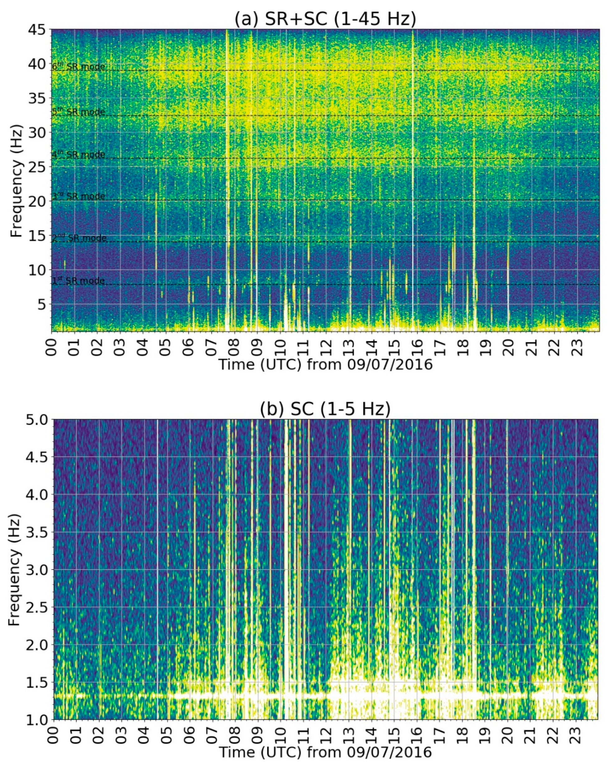
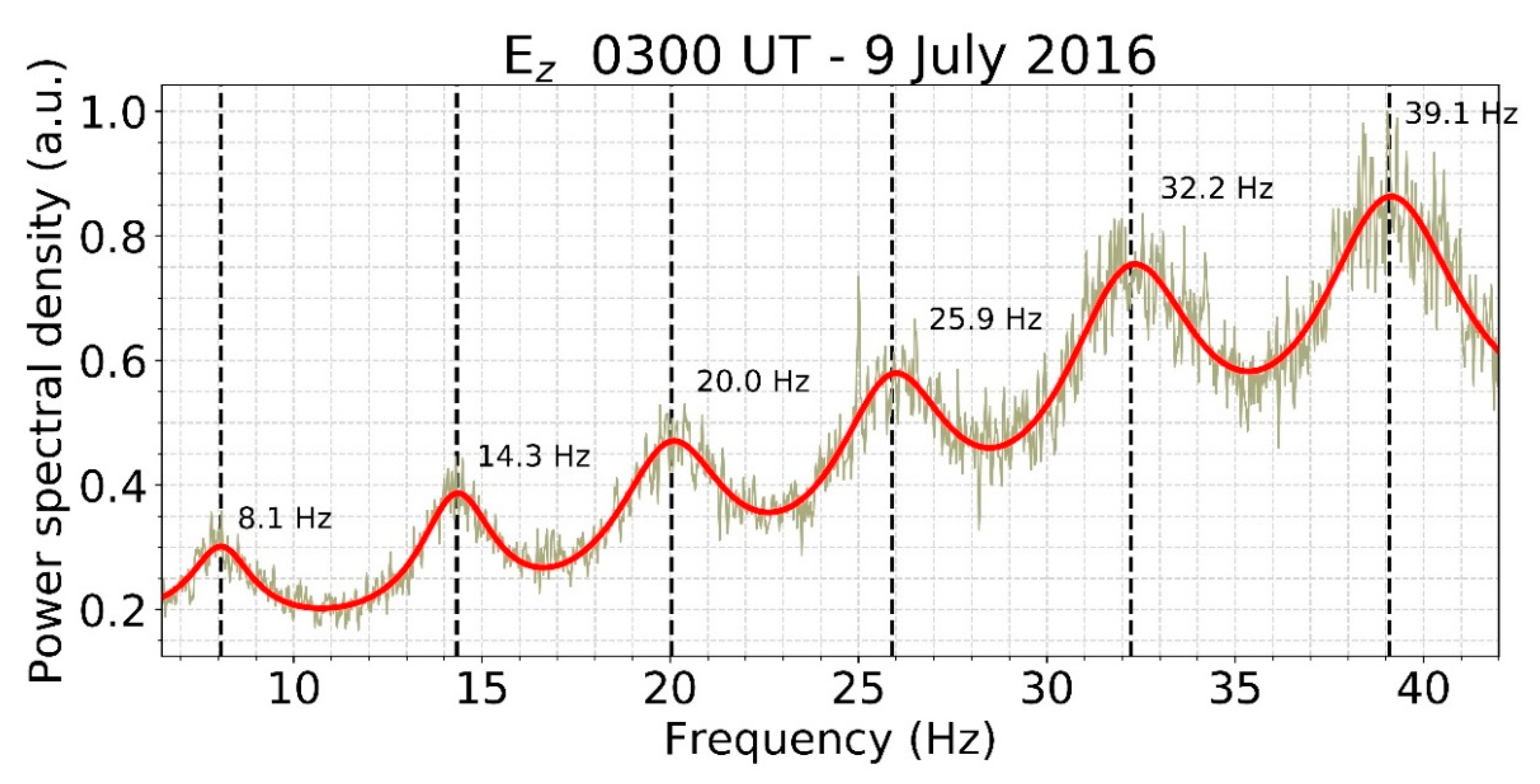
2.2. Data Processing

The digitized raw data are collected every 15-min (90,000 samples taken with 100 Hz sampling frequency) and stored locally in binary format. Each sample contains a series of information including system status, timestamp, and signal amplitude. The time-series of antenna output are used in this specific case to obtain the spectrograms and amplitude spectra described in Section 3.1. The long-term analysis is rather based upon stats files that are generated from the raw data for the period from 1 June 2015 to 31 May 2020. In this case, the raw data are filtered using a six-pole Butterworth bandpass filter to separate SC motion (1–5 Hz) from global lightning (10–45 Hz) (i.e., selecting the first and higher SR harmonics and suppressing lower frequency noise), before computing summary statistics (i.e., min/max, mean, standard deviation) for the antenna output on 15-min time periods. The standard deviation (hereafter SD) is specifically used as a measure of the SR cumulative intensity in that bandwidth, after showing that SR dominate the displacement current spectrum in fair-weather at those frequencies (Section 3.1). Locally disturbed conditions are filtered out by rejecting SD values larger than a maximum threshold of 12 pA. The SD, in fact, significantly increases by several orders of magnitude in disturbed weather (~tens of nA), due mainly to tropospheric sources such as precipitation and local lightning or in the presence of local interference. Nevertheless, disturbed weather samples and missing data constitute at most less than about 10% of the 5-year total observation time.

3. Results and Discussion

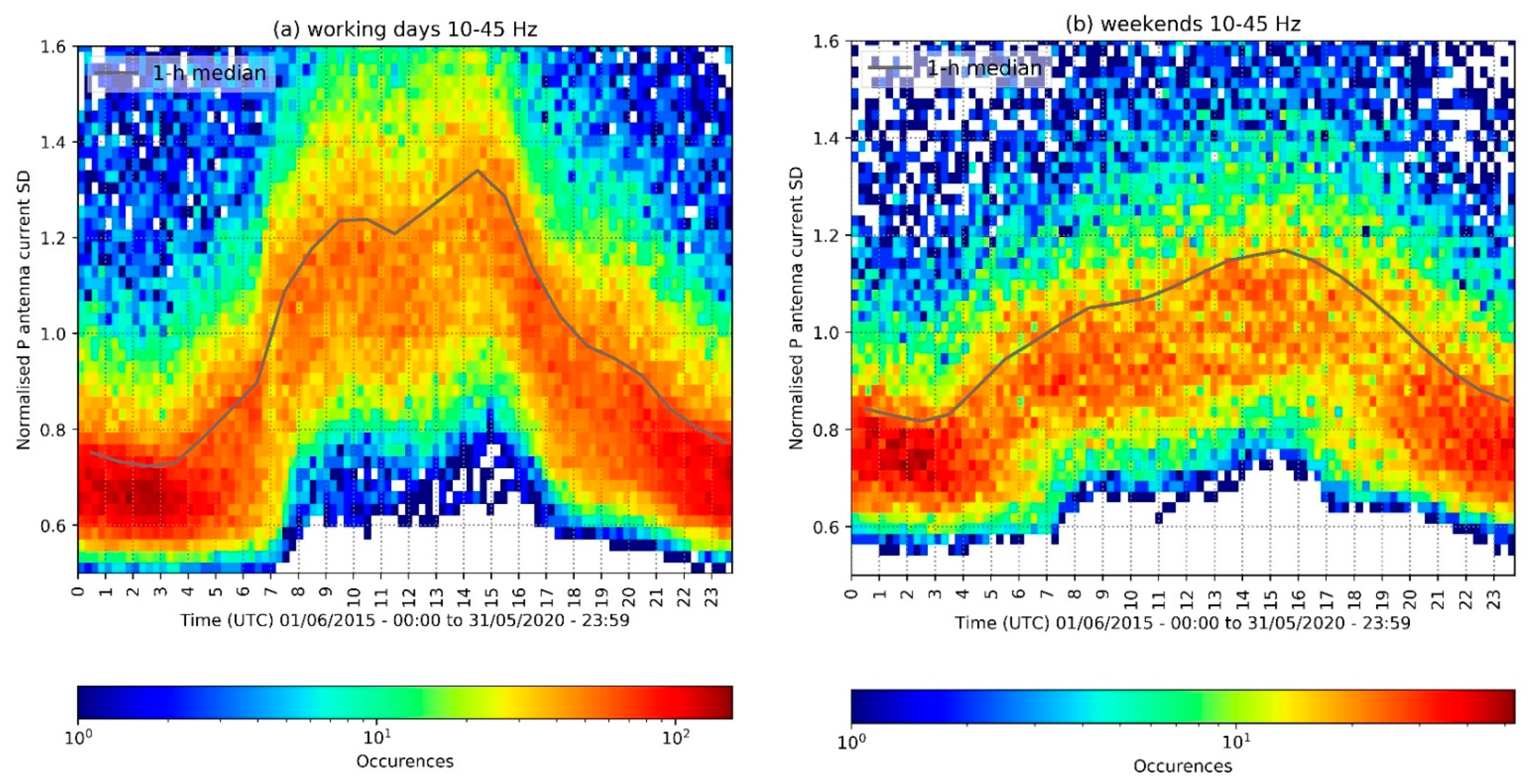
3.1. Displacement Current Sources in Fair-Weather

The analysis of the raw data is initially made in the frequency domain to identify the dominant natural sources of background variability in the 1-45 Hz electric field. Dynamic spectrograms using the Welch method [27] are created for sample fair-weather days from midnight (00 UT) to midnight of the following day. The Welch’s method computes an estimate of the power spectral density by dividing the data into overlapping segments, computing a modified periodogram for each segment, and averaging the periodograms. Daily spectrograms are computed using 100 s (10,000 points) intervals of filtered data and applying a 4096-points Fourier transform to produce 864 1-D spectra plots per day. Figure 2 shows an example of a spectrogram (frequency window: 1–45 Hz) from 9 July 2016. The SR modes are resolved in this graph as persistent horizontal bands of enhanced power centred roughly around 8, 14, 20, 26, 32, and 38 Hz (Figure 2a). SR can therefore be considered as a major source of output current in fair weather, aside from local turbulent SC which instead largely dominates below 5 Hz (Figure 2b). The SC effect is largely dependent on surface wind speed and influenced by different weather conditions. Yet, it can increase during advection of pollutants from surrounding cities and sea salt aerosols at the site. The variability of 1–3 Hz band of the antenna current was previously used as a proxy for near-surface turbulence during March 2015 solar eclipse by Bennett [28]. Some additional transient disturbances are visible as thin vertical lines. These artifacts are normally associated with occasional high amplitude but short duration noise from charged feathers of birds flying nearby the sensor or electrical interference at the installation site.
A typical example of the SR electric component raw amplitude spectrum taken from the BTD is given in Figure 3. The spectrum is computed using an FFT algorithm on filtered data in the frequency interval 5–45 Hz. The SR peaks up to the 6th mode are distinctly detected in fair weather and in the absence of relevant manmade interference. The principal parameters of each mode, such as modal frequency and relative peak amplitude, can be estimated by least-squares fitting of the experimental spectrum with the sum of 6 Lorentzian functions (red line in Figure 3) of the form:
A i ( f ) = A i   [ ( f f i ) ω i ] 2 + 1 ,
where Ai is the amplitude of mode i as a function of frequency f, fi the central frequency of mode i and ωi the half-width of mode i in Hz, in analogy to the method used by Price and Melnikov [12].
As anticipated, the main aim of this research is to study the diurnal and long-term variability of the SR signal, related primarily to the diurnal/seasonal cycle of global thunderstorm activity. Unlike the majority of SR-related studies, however, the possibility to use the time-series of 15-min antenna current SD in the 10–45 Hz band as a measure of the SR cumulative intensity variation rather than the SR peak parameters are examined in the following sections. The chosen filter bandwidth implies the disadvantage of cutting off the SR fundamental frequency. Nevertheless, this does not invalidate the results presented, since it allows to avoid lower frequency noise at the installation site, which could eventually affect the first mode most.

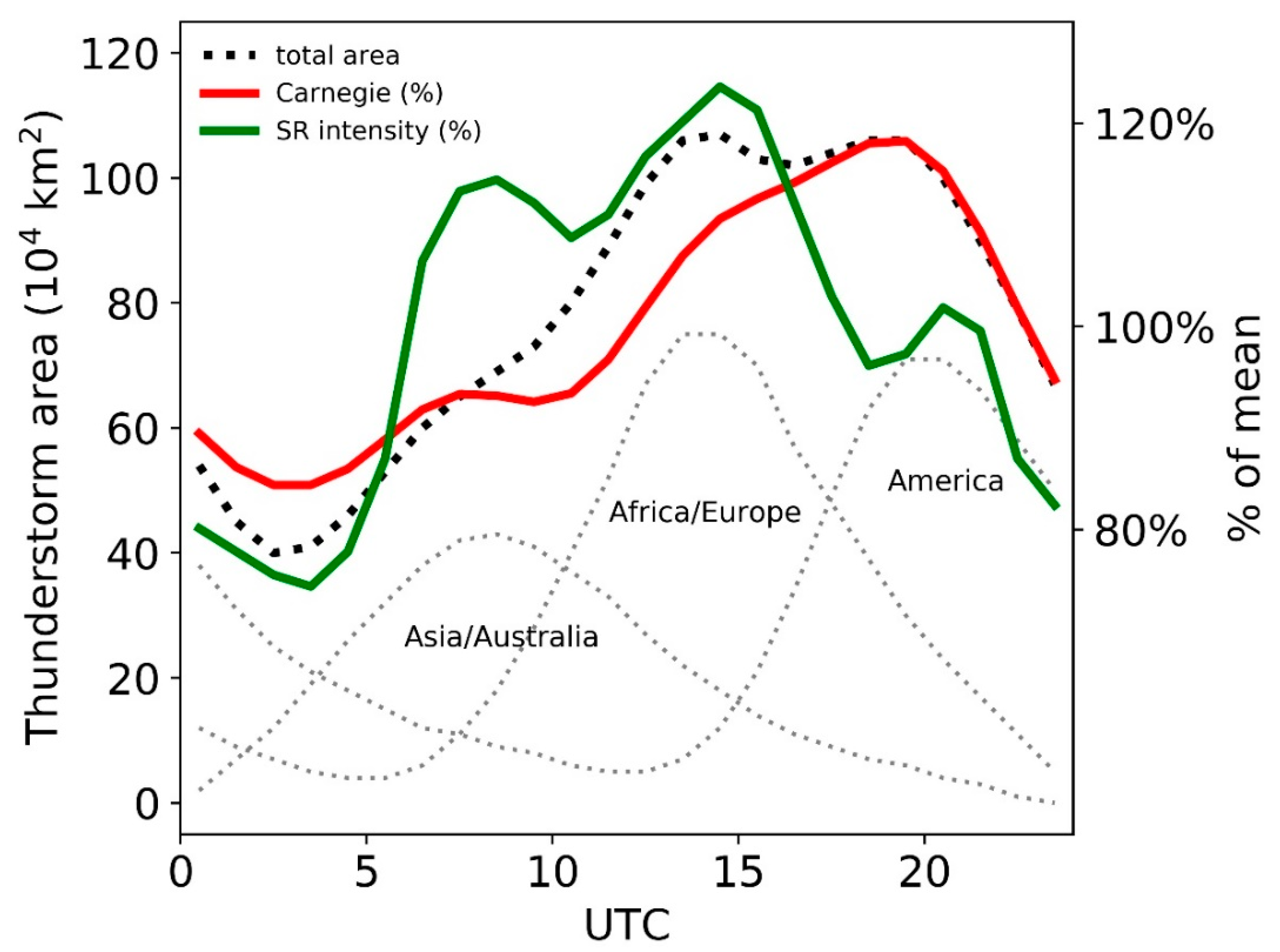
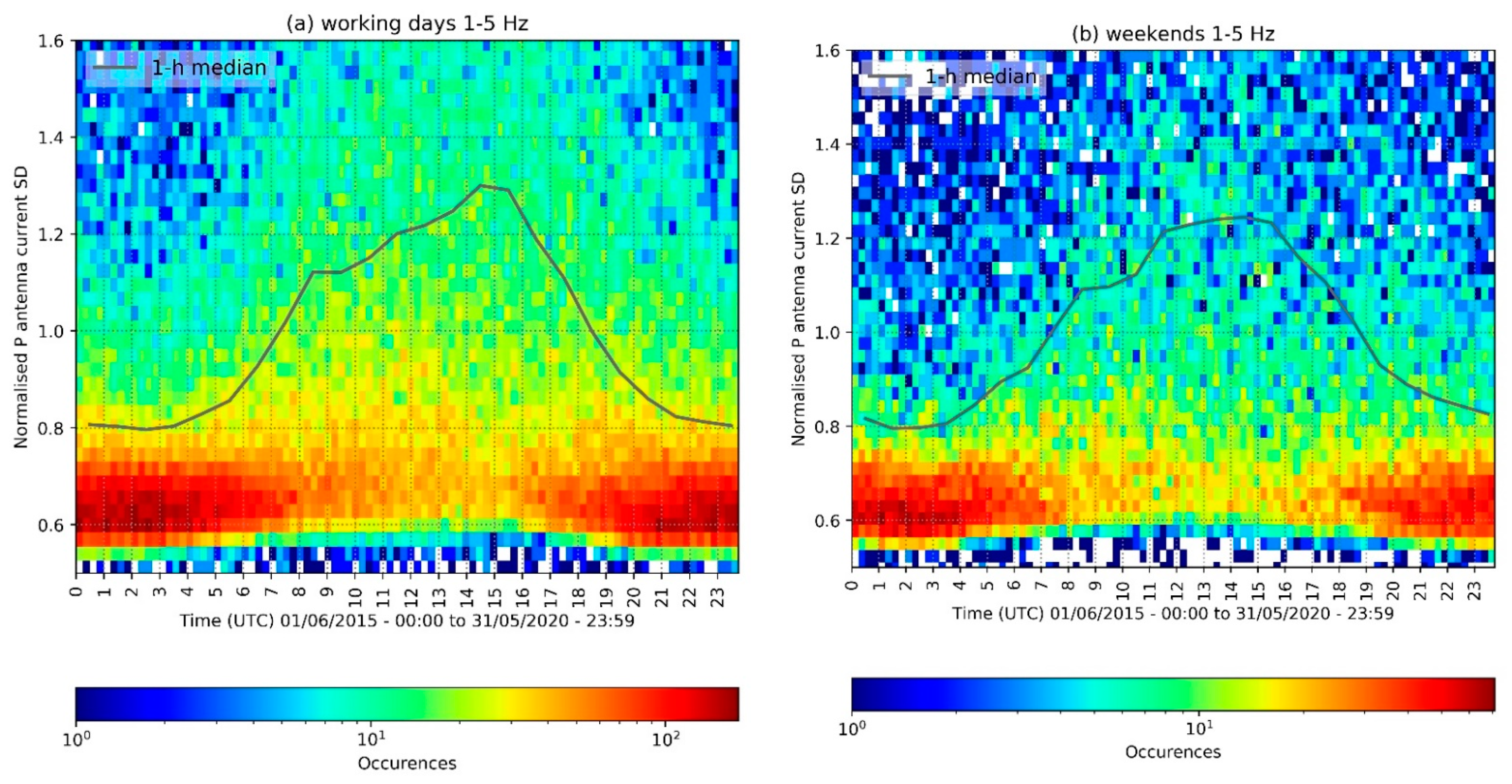
3.2. Diurnal Variation

The electric component of SR, which is the source of the antenna output, is independent of the direction of the source relative to the observer. A typical SR diurnal record hence reflects the properties of both global thunderstorm activity, although biased by the SOD, and in a smaller measure the state of the Earth-ionosphere cavity between the source region and the observer. The diurnal cycle of the 10–45 Hz frequency band is shown as a density plot in Figure 4, that distinguishes between working days (a) and weekends only (b). During the daylight period, the ionospheric profile would be relatively constant, so the change in SR magnitude is considered representative of the strength of global thunderstorms. In general, both cases illustrate that, in analogy to SR, the diurnal SD variation increases at early morning hours, in response to the development of thunderstorm activity in southeast Asia and Oceania, which is peaked at around 09 UT. The SD increase reaches its maximum peak at around 15–16 UT, coinciding with the maximum lightning activity of the African centre. The overall amplitude of the signal from the Amazon basin and South America in the evening hours (20–21 UT) is typically less pronounced during most of the year at the observation site. Yet, it becomes more evident in the winter season of the northern hemisphere, when the influence of European thunderstorm activity is low. The reduced strength of the SR power during the night is in general attributed to a reduction in the global thunderstorm activity during the time when the sun passes over the Pacific. Given the time coincidence between the observed diurnal trend of SR power and the day-night terminator, past studies also investigated the possible influence of variations of the ionosphere (i.e., the upper waveguide boundary) on SR, suggesting a modulation by the dynamic local ionospheric height [29]. Later studies, though, estimated the effect of diurnal ionospheric changes on the amplitude of the SR fundamental frequency in about ~10% with respect to a uniform model [30], indicating that diurnal and seasonal changes in the source properties are the primary drivers.
It is worth noticing that anthropogenic disturbances at the installation site during working days determine an increased variability of the SD amplitude during the daytime that superimposes to the global lightning effect, which is hence better represented by weekend data (i.e., no ongoing activity in the building). This influence is particularly pronounced during working hours (07–17 UT). Its removal by considering weekends data only is beneficial to better characterize the seasonal and long-term variability.
The same output for the 1–5 Hz band is shown in Figure 5, which represents the nearby windblown charge band. The median SC diurnal fluctuations are essentially associated with changing tropospheric conditions during the typical day and less sensitive to other types of manmade disturbances. In particular, calmer and more stable wind conditions on average during the night reduce the amount of turbulence near the BTD, causing a reduction in windblown charge. This is shown in Figure 5, where the 1–5 Hz band has a consistently low variability between 2100 UTC and 0600 UTC, before increasing and becoming considerably more variable in response to greater mixing during the daytime.
In Figure 6, the diurnal variation of the SD of current induced on the antenna in the 10–45 Hz is presented for each season in the 5-year observation time. Similarly to the results found in previous studies, each season exhibits a specific pattern likely resulting from the dynamics of the north-south seasonal migration of global lightning, that is reproducible through the period considered. Minor differences in the peak amplitude are attributable to inter-annual variability in climate drivers, such as convective activity and lightning intensity changes in specific areas of the globe in response to the trend of global temperatures, as shown in Section 3.3. In general, the seasonal plots in Figure 6 illustrate some anticipated features, such as the minimum around 2–4 UT and a peak activity centred between 14–16 UT, determined by the African lightning chimney because of the relatively shorter SOD. Yet, substantial differences emerge that highlight the site-dependent SR measurement response to the seasonal shifts in the major lightning centres. The summer (JJA) diurnal pattern exhibits a single oscillation, culminating at about 18 UT. This may suggest a possible distortion from mid-latitude lightning activity in Europe during the northern hemisphere summer, potentially obscuring additional oscillations that are instead observed during the other seasons. In particular, the diurnal oscillations in the cumulative SR intensity [14] are more pronounced during winter months (DJF), when European thunderstorm activity is at a minimum [31]. Additionally, a higher correlation is found in SON-DJF months (0.94 and 0.92, respectively) compared with JJA months (0.85) for diurnal SD (Portishead)-diurnal SR (NCK), as highlighted in Table 1.
A comparison versus the working days’ output is shown in Figure 7, where seasonal diurnal changes are superimposed to increased daytime variability from surrounding manmade interference. Each season well reproduces the expected diurnal features, notably the dominant afternoon peak (15 UT), but relevant differences are also found with respect to the weekend dataset. In particular, the influence of cultural noise on the diurnal SD amplitude appears more pronounced at morning hours, causing a systematic shift forward on average of the morning peak (~8 UT) relative to the reference SR measurements at NCK and the weekend data.

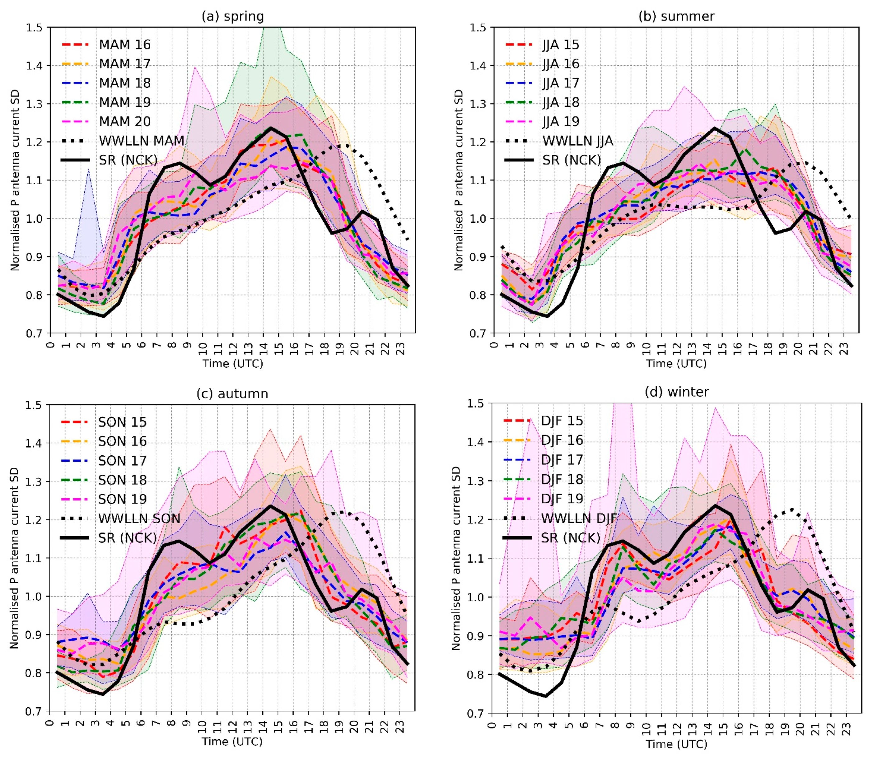
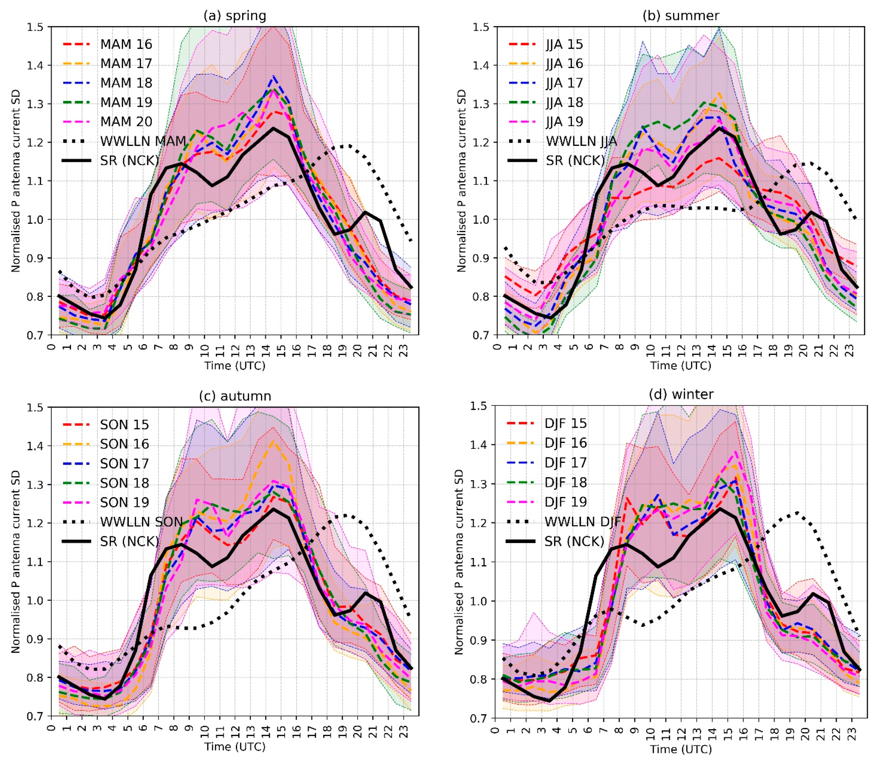
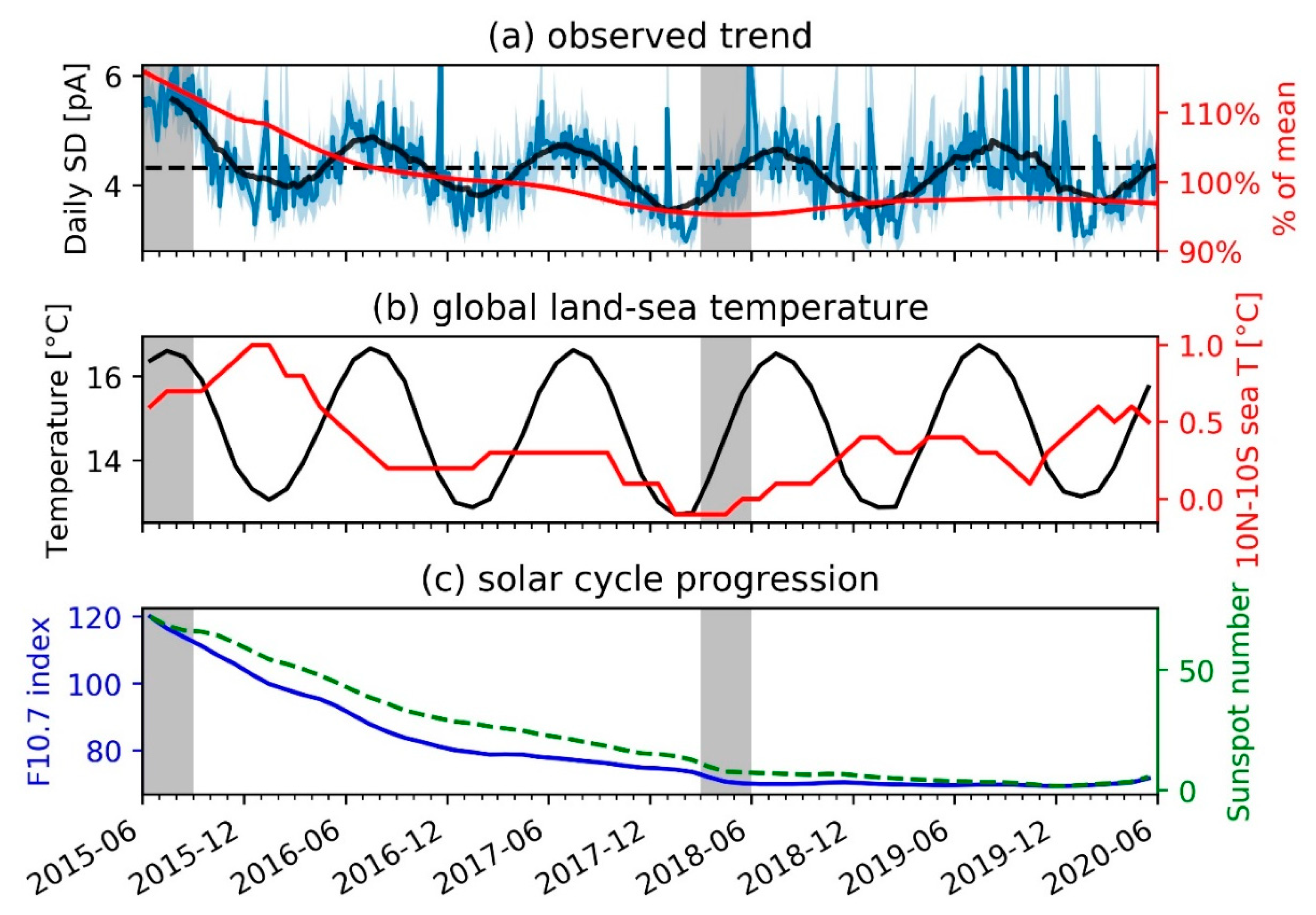
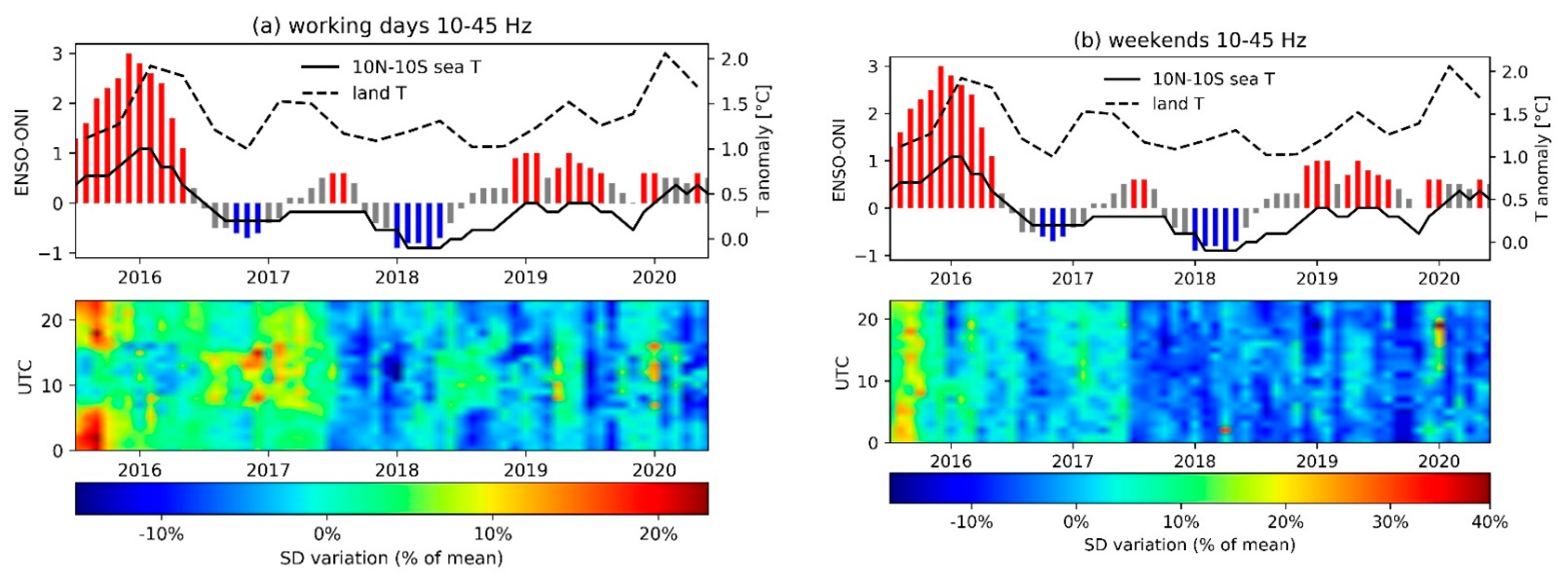
3.3. Combined Annual and Inter-Annual Variation

The presence of SR power and frequency inter-annual variability has been found to emerge from a complex interplay of global land-ocean temperature changes, related convective rainfall and lightning intensity variation, and the solar cycle progression. Evidence of such long-term modulation is clearly seen also from the BTD measurements taken at Portishead. Figure 8 shows the observed trend in the daily antenna median SD amplitude, represented as the blue solid line which is superimposed to the interquartile range calculated for each day (light blue shaded area). The rolling mean, calculated with a 30-point window convolution filter (black line), exhibits an unambiguous annual oscillation that is a manifestation of the annual global surface air temperature (Figure 8b) changes (~1.5–2 °C) determining variation with the same period in the global lightning activity, and accordingly in the SR signal amplitude. The maximum peak in the SD occurs during the northern hemisphere summer (JJA), where most of the continental landmasses are distributed, and coincides with the maximum lightning intensity recorded globally [33]. Hayakawa et al. [34] reported a strong correlation between periodic variations of SR intensity recorded at Moshiri (Japan) and global surface temperature in the ±45° latitude band. Similarly, the BTD output signal in the SR band is found to oscillate in-phase with the combined global land-sea temperature from NOAA’s National Climatic Data Center, indicating a cross-correlation coefficient of about 0.9, that is consistent with the result found by Sekiguchi et al. [35] using magnetic field data. Yet, it is worth noticing that the SD amplitude annual oscillations are not stationary but show evidence of an overlapped inter-annual trend. This trend is extracted from the SD daily medians, applying a seasonal decomposition technique [36] to decompose the time series into three additive components (trend, seasonal and residual). The observed inter-annual trend (solid red line in Figure 8a) decreases between June 2015 and June 2018, which corresponds to the SD extrema (maximum and minimum, respectively) recorded during the 5-year period, and subsequently becomes nearly constant. An exceptional increase of the SR intensity for the period 2015/2016 has been documented by other studies, that considered the SR modes average peak frequency and intensity measured at various observatories distributed globally [20,24,37]. In analogy with other SR amplitude observations taken at similar mid-high latitudes (i.e., Eskdalemuir [25]), the steady decline in the inter-annual SD is found to be in phase with the transition from the maximum to the minimum of the 11-year solar cycle (Figure 8c). Satellite observations do not show a solar phase-related variation in the intensity and distribution of global thunderstorm activity (i.e., the primary origin of SR) [38]. Solar cycle-related long-term changes in the SR frequency and power are thus attributed to the modification of the earth-ionosphere medium, and in particular to a reduction of local ionospheric height resulting from increased solar X-rays and energetic electron precipitation (EEP) near to periods of maximum solar activity [37,39]. In the absence of data covering an entire solar cycle, however, a univocal interpretation of the long-term trend observed in the BTD data is still challenging. Intrinsic source changes associated with other global climate drivers may in fact play a significant role in the inter-annual SR variability observed worldwide. A qualitative agreement is actually found when looking at the evolution of the 10 N–10 S ocean temperature anomaly for the same period (Figure 8b), indicating a possible SR (and in turn the antenna current) response to global climate effects on major lightning sources.
In this regard, Williams [18] found a significant positive correlation between the relative tropical temperatures during an El Niño cycle and the amplitude of the SR fundamental frequency, suggesting a complex modulation of the lightning flash rate by global temperature changes. Several later works investigated the inter-annual changes in SR parameters on the basis of the ENSO (El Niño Southern Oscillation) phenomenon which can change the global atmospheric circulation, and in turn, affect the weather pattern around the world [40,41,42]. In particular, most of them considered the influence of sea surface temperature (SST) anomalies in the Pacific Ocean under warm and cold ENSO phases as a source of spatial shifts of the thunderstorm regions globally, thus affecting the measured SR intensity at a given observing station. More recently, Williams et al. [20] investigated this idea further by making use of SR data from multiple recording stations worldwide. They found a considerable increase of the 1st SR mode intensity in the transition months preceding the peak in two super El Niño events (1997/1998 and 2015/2016), associated with an increase in lightning activity observed from independent satellite and ground observations. This is attributed to increased instability due to thermodynamic imbalance between the surface and the mid-troposphere at the transition. In Figure 9b the long-term SD relative variation recorded by the antenna is shown and compared to the Oceanic Niño Index (ONI) (3 months running mean of ERSST.v5 SST anomalies in the Niño 3.4 region (5 N–5 S, 120–170 W), based on centred 30-year base periods updated every 5 years). Warm and cold ENSO episodes are classified as such when a threshold of ±0.5 °C above or below the normal SST is met for at least 5 consecutive overlapping seasons. This approach highlights the months and the UT time characteristics of the SD magnitude anomalies. In order to emphasize the effect of long-term climate changes, diurnal and seasonal influence on the data is removed by calculating the monthly average diurnal variation of the SD with 1-h time resolution (i.e., a 24 × 12 matrix characterises each processed year) and then normalising each bin value (SDi) by the 5-year average for the specific time and month (SDi,avg) as follows:
S D i , n o r m ( % ) = S D i S D i , a v g S D i , a v g 100 ,
The patterns seen in the time-UT anomalies of SD amplitude plot for the 10–45 Hz band show a noticeable increase (~20–30% of the mean) during the summer months of 2015, while approaching the peak of the exceptional 2015–2016 warm ENSO episode, which culminated in the maximum ocean temperature anomaly recorded for the entire period considered. The subsequent decrease to values lower than about 0.5 °C in the 10 N–10 S SST anomaly, coincided with a substantial transition to negative SD anomalies, which is particularly evident from the second half of 2017, during the months that preceded the 2018 cold ENSO phase. Similar enhancements/diminutions in the SD amplitude would require more specific analysis, combining measurements from other observatories and including global convective rainfall and lightning data. Yet, if confirmed by future studies, the amplitude and time of occurrence of such anomalies in the SD may be used as a proxy of complex global scale relationships with ENSO, revealing changes in lightning frequency and distribution pattern in specific areas of the globe. The necessity of choosing an ideal site for such measurements is further highlighted in Figure 9a, where it is shown that the increased daytime local variability during working hours may mask eventual diurnal SD anomalies otherwise seen in the weekend data. Such effect is observed, for example, during JJA 15.

4. Conclusions

The BTD-300 sensor installed at Portishead (UK), has proved its ability to detect and monitor the Schumann resonances at a single site on a permanent basis, even in an urban environment where manmade interference during working hours may not be negligible. The data presented in this work are a valuable reference in atmospheric electricity studies, as they represent the first continuous survey of SR effects in the electric field component from the UK since 2015, helping also in characterising site-specific environment influence on the SR measurements.
The method of data acquisition and processing can provide both principal SR mode parameters (peak frequencies and amplitudes) for at least the first six SR modes and additional quantities (i.e., displacement current SD), useful as a proxy of the cumulative SR power in the 10–45 Hz frequency band. These latter data, collected during the 5 years of observations 2015/2020, are analysed and presented in various graphical forms to point out eventual SR intensity changes on a diurnal, seasonal, and inter-annual basis.
Measurements at Portishead qualitatively confirm the overall pattern of diurnal and seasonal variations in SR amplitudes as reported from other observatory sites, confirming that the changes in source-observer distance are dominant for seasonal variations in the diurnal pattern, with the African chimney being prevailing through most of the year at this specific site.
Recorded inter-annual variations in SD amplitude are better explained in terms of SR response to a complex interplay of solar cycle progression and climate variables leading to a modulation of global lightning intensity, not limited to only the 3 major lightning hotspots on Earth. This has been confirmed by preliminary agreement found with previous studies linking SR to global climate indexes as the SST anomaly and trend in the global land-sea temperature. Yet, a concurrent role played by the 11-year solar cycle in determining the observed inter-annual SD trend cannot be ruled out. The still ongoing data collection would certainly be beneficial in consolidating these findings, especially if (1) additional comparisons with other observatories will be made, (2) future measurements will be conducted at sites less affected by cultural noise, (3) the equipment will be improved for future application in SR research.

Author Contributions

Conceptualization, A.P., A.B. and M.F.; methodology, A.P. and A.B.; software, A.P. and A.B.; validation, A.B. and M.F.; formal analysis, A.P.; investigation, A.P. and A.B.; data curation, A.P. and A.B.; writing—original draft preparation, A.P.; writing—review and editing, A.P.; supervision, A.B. and M.F. All authors have read and agreed to the published version of the manuscript.

Funding

The work of A.P. is supported by the European Union’s Horizon 2020 research and innovation programme under the Marie Sklodowska-Curie grant agreement 722337.

Institutional Review Board Statement

Not applicable.

Informed Consent Statement

Not applicable.

Data Availability Statement

Data used in this study are made available upon request to the corresponding author.

Acknowledgments

The authors thank Alexander P. Nickolaenko and one anonymous reviewer for a comprehensive review of the manuscript and suggestions for improvement and future works. The authors are also grateful to José Tacza for providing the WWLLN thunderstorm days estimation used as a reference in the manuscript.

Conflicts of Interest

The authors declare no conflict of interest. The funders had no role in the design of the study; in the collection, analyses, or interpretation of data; in the writing of the manuscript, or in the decision to publish the results.

References

  1. Schumann, W.O. Über die Dämpfung der elektromagnetischen Eigenschwingungen des Systems Erde—Luft—Ionosphäre. Z. Für Nat. A 1952, 7, 250–252. [Google Scholar] [CrossRef]
  2. Füllekrug, M. Detection of thirteen resonances of radio waves from particularly intense lightning discharges. Geophys. Res. Lett. 2005, 32, L13809. [Google Scholar] [CrossRef] [Green Version]
  3. Füllekrug, M.; Constable, S. Global triangulation of intense lightning discharges. Geophys. Res. Lett. 2000, 27, 333–336. [Google Scholar] [CrossRef]
  4. Surkov, V.V.; Hayakawa, M. Schumann resonances excitation due to positive and negative cloud-to-ground lightning. J. Geophys. Res. 2010, 115, D04101. [Google Scholar] [CrossRef]
  5. Chapman, F.W.; Jones, D.L.; Todd, J.D.W.; Challinor, R.A. Observations on the Propagation Constant of the Earth Ionosphere Waveguide in the Frequency Band 8 c/s to 16 kc/s. Radio Sci. 1966, 1, 1273–1282. [Google Scholar] [CrossRef]
  6. Ogawa, T.; Tanaka, Y.; Miura, T.; Yasuhara, M. Observations of Natural ELF and VLF Electromagnetic Noises by Using Ball Antennas. J. Geomagn. Geoelectr. 1966, 18, 443–454. [Google Scholar] [CrossRef]
  7. Füllekrug, M. Schumann resonances in magnetic field components. J. Atmos. Terr. Phys. 1995, 57, 479–484. [Google Scholar] [CrossRef]
  8. Bozóki, T.; Prácser, E.; Sátori, G.; Dálya, G.; Kapás, K.; Takátsy, J. Modeling Schumann resonances with schupy. J. Atmos. Sol.-Terr. Phys. 2019, 196, 105144. [Google Scholar] [CrossRef] [Green Version]
  9. Balser, M.; Wagner, C.A. Observations of Earth-Ionosphere Cavity Resonances. Nature 1960, 188, 638–641. [Google Scholar] [CrossRef]
  10. Sátori, G. Monitoring schumann resonances-11. Daily and seasonal frequency variations. J. Atmos. Terr. Phys. 1996, 58, 1483–1488. [Google Scholar] [CrossRef]
  11. Nickolaenko, A.P.; Sátori, G.; Zieger, B.; Rabinowicz, L.M.; Kudintseva, I.G. Parameters of global thunderstorm activity deduced from the long-term Schumann resonance records. J. Atmos. Sol.-Terr. Phys. 1998, 60, 387–399. [Google Scholar] [CrossRef]
  12. Price, C.; Melnikov, A. Diurnal, seasonal and inter-annual variations in the Schumann resonance parameters. J. Atmos. Sol.-Terr. Phys. 2004, 66, 1179–1185. [Google Scholar] [CrossRef]
  13. Sekiguchi, M.; Hobara, Y.; Hayakawa, M. Diurnal and seasonal variations in the Schumann resonance parameters at Moshiri, Japan. J. Atmos. Electr. 2008, 28, 1–10. [Google Scholar] [CrossRef]
  14. Sátori, G.; Mushtak, V.; Williams, E. Schumann Resonance Signatures of Global Lightning Activity. In Lightning: Principles, Instruments and Applications; Springer: Dordrecht, The Netherlands, 2009; pp. 347–386. [Google Scholar] [CrossRef]
  15. Zhou, H.; Yu, H.; Cao, B.; Qiao, X. Diurnal and seasonal variations in the Schumann resonance parameters observed at Chinese observatories. J. Atmos. Sol.-Terr. Phys. 2013, 98, 86–96. [Google Scholar] [CrossRef]
  16. Whipple, F.J.W. On the association of the diurnal variation of electric potential gradient in fine weather with the distribution of thunderstorms over the globe. Q. J. R. Meteorol. Soc. 1929, 55, 1–18. [Google Scholar] [CrossRef]
  17. Harrison, R.G. The Carnegie Curve. Surv. Geophys. 2013, 34, 209–232. [Google Scholar] [CrossRef] [Green Version]
  18. Williams, E.R. The Schumann Resonance: A Global Tropical Thermometer. Science 1992, 256, 1184–1187. [Google Scholar] [CrossRef] [PubMed]
  19. Sátori, G.; Williams, E.; Lemperger, I. Variability of global lightning activity on the ENSO time scale. Atmos. Res. 2009, 91, 500–507. [Google Scholar] [CrossRef]
  20. Williams, E.; Bozóki, T.; Sátori, G.; Price, C.; Steinbach, P.; Guha, A.; Liu, Y.; Beggan, C.D.; Neska, M.; Boldi, R.; et al. Evolution of Global Lightning in the Transition From Cold to Warm Phase Preceding Two Super El Niño Events. J. Geophys. Res. Atmos. 2021, 126, e2020JD033526. [Google Scholar] [CrossRef]
  21. Nickolaenko, A.P.; Koloskov, A.V.; Hayakawa, M.; Yampolski, Y.M.; Budanov, O.V.; Korepanov, V.E. 11-year solar cycle in Schumann resonance data as observed in Antarctica. Sun Geosph. 2015, 10, 39–49. [Google Scholar]
  22. Manu, S.; Rawat, R.; Sinha, A.K.; Gurubaran, S.; Jeeva, K. Schumann resonances observed at Maitri, Antarctica: Diurnal variation and its interpretation in terms of global thunderstorm activity. Curr. Sci. 2015, 109, 784–790. [Google Scholar]
  23. Beggan, C.; Allmark, C.; Swan, A.; Flower, S.; Thomson, A. Investigation of global lightning using Schumann resonances measured by high frequency induction coil magnetometers in the UK. In Proceedings of the National Astronomy Meeting of the Royal Astronomical Society, St. Andrews, UK, 1–5 July 2013. [Google Scholar]
  24. Musur, M.A.; Beggan, C.D. Seasonal and Solar Cycle Variation of Schumann Resonance Intensity and Frequency at Eskdalemuir Observatory, UK. Sun Geosph. 2019, 14, 81–86. [Google Scholar] [CrossRef]
  25. Bennett, A.J. Electrostatic thunderstorm detection. Weather 2017, 72, 51–54. [Google Scholar] [CrossRef]
  26. Bennett, A.J. Identification and ranging of lightning flashes using co-located antennas of different geometry. Meas. Sci. Technol. 2013, 24, 125801. [Google Scholar] [CrossRef]
  27. Welch, P. The use of fast Fourier transform for the estimation of power spectra: A method based on time averaging over short, modified periodograms. IEEE Trans. Audio Electroacoust. 1967, 15, 70–73. [Google Scholar] [CrossRef] [Green Version]
  28. Bennett, A.J. Effects of the March 2015 solar eclipse on near-surface atmospheric electricity. Philos. Trans. R. Soc. A Math. Phys. Eng. Sci. 2016, 374, 20150215. [Google Scholar] [CrossRef]
  29. Sentman, D.D.; Fraser, B.J. Simultaneous observations of Schumann resonances in California and Australia: Evidence for intensity modulation by the local height of the D-region. J. Geophys. Res. Space Phys. 1991, 96, 15973–15984. [Google Scholar] [CrossRef]
  30. Pechony, O.; Price, C.; Nickolaenko, A.P. Relative importance of the day-night asymmetry in Schumann resonance amplitude records. Radio Sci. 2007, 42, RS2S06. [Google Scholar] [CrossRef] [Green Version]
  31. Taszarek, M.; Allen, J.; Pucik, T.; Groenemeijer, P.; Czernecki, B.; Kolendowicz, L.; Lagouvardos, K.; Kotroni, V.; Schulz, W. A Climatology of Thunderstorms across Europe from a Synthesis of Multiple Data Sources. J. Clim. 2019, 32, 1813–1837. [Google Scholar] [CrossRef]
  32. Ccopa, J.G.A.; Tacza, J.; Raulin, J.-P.; Morales, C.A. Estimation of thunderstorms occurrence from lightning cluster recorded by WWLLN and its comparison with the “universal” Carnegie curve. J. Atmos. Sol.-Terr. Phys. 2021, 221, 105682. [Google Scholar] [CrossRef]
  33. Cecil, D.J.; Buechler, D.E.; Blakeslee, R.J. Gridded lightning climatology from TRMM-LIS and OTD: Dataset description. Atmos. Res. 2014, 135–136, 404–414. [Google Scholar] [CrossRef] [Green Version]
  34. Hayakawa, M.; Sekiguchi, M.; Hobara, Y.; Nickolaenko, A.P. Intensity of Schumann resonance oscillations and the ground surface temperature. J. Atmos. Electr. 2006, 26, 79–93. [Google Scholar] [CrossRef]
  35. Sekiguchi, M.; Hayakawa, M.; Nickolaenko, A.P.; Hobara, Y. Evidence on a link between the intensity of Schumann resonance and global surface temperature. Ann. Geophys. 2006, 24, 1809–1817. [Google Scholar] [CrossRef] [Green Version]
  36. Cleveland, R.B.; Cleveland, W.S.; McRae, J.E.; Terpenning, I. STL: A Seasonal-Trend Decomposition Procedure Based on LOESS. J. Off. Stat. 1990, 6, 3–73. [Google Scholar]
  37. Bozóki, T.; Sátori, G.; Williams, E.; Mironova, I.; Steinbach, P.; Bland, E.C.; Koloskov, A.; Yampolski, Y.M.; Budanov, O.V.; Neska, M.; et al. Solar Cycle-Modulated Deformation of the Earth-Ionosphere Cavity. Front. Earth Sci. 2021, 9, 735. [Google Scholar] [CrossRef]
  38. Christian, H.J. Global frequency and distribution of lightning as observed from space by the Optical Transient Detector. J. Geophys. Res. 2003, 108, ACL 4-1–ACL 4-15. [Google Scholar] [CrossRef]
  39. Sátori, G.; Williams, E.; Mushtak, V. Response of the Earth-ionosphere cavity resonator to the 11-year solar cycle in X-radiation. J. Atmos. Sol.-Terr. Phys. 2005, 67, 553–562. [Google Scholar] [CrossRef]
  40. Füllekrug, M.; Fraser-Smith, A.C. Global lightning and climate variability inferred from ELF magnetic field variations. Geophys. Res. Lett. 1997, 24, 2411–2414. [Google Scholar] [CrossRef]
  41. Sátori, G.; Zieger, B. El Niňo related meridional oscillation of global lightning activity. Geophys. Res. Lett. 1999, 26, 1365–1368. [Google Scholar] [CrossRef]
  42. Yang, H.; Pasko, V.P. Power variations of Schumann resonances related to El Niño and La Niña phenomena. Geophys. Res. Lett. 2007, 34, L11102. [Google Scholar] [CrossRef] [Green Version]
Figure 1. Comparison of the diurnal UT variations of thunderstorm surface area worldwide [16] and the UT variation of electric potential gradient over the ocean (Carnegie curve), calculated as percentage of the mean using annual values reported in Harrison [17]. The cumulative relative intensity of the first three SR modes of the Ez field component observed at Nagycenk (NCK), Hungary, for the period 1994–1998, follows a similar general diurnal trend and exhibits three maxima which correspond to the three major sources of tropical thunderstorms. The peaks in the SR amplitude are better resolved in autumn and winter, when the influence from local thunderstorm activity at the observatory is lower [14].
Atmosphere 13 00038 g001
Figure 2. Daily spectrogram of 100 Hz output current from the spherical antenna at Portishead during 6 July 2016, with spectra calculated every 100 s. The major contribution to fair-weather current is given by a combination of turbulent space charge (SC) motion (<5 Hz) and global SR signal (>5 Hz), the latter visible as a series of diffuse horizontal bands corresponding to each SR mode frequency that falls within the antenna range (1–45 Hz) (panel (a)). Superimposed vertical lines originate from occasional transient local disturbances. Panel (b) magnifies the SC effect and indicates that this is at a minimum during late night but largely increases after 0500 UT, hence the need to remove potential data contamination when looking at the SR variability.
Atmosphere 13 00038 g002
Figure 3. Typical raw spectrum of the output current, depending on the electric component of SR signal, measured at Portishead at 0300 UT on 9 July 2016, under favourable conditions. The spectrum is fitted with a sum of 6 Lorentzian functions (red line) and the peak frequency of each mode, determined by the best fit parameters, is shown. The rise of power with frequency is caused by the specific response function of the sensor.
Atmosphere 13 00038 g003
Figure 4. Diurnal variation of the standard deviation of current induced on the antenna in the 10–45 Hz frequency range (1 June 2015–31 May 2020) during (a) working days (Mon–Fri) and (b) weekends only (Sat–Sun), represented as a 2-D histogram with 15-min temporal resolution (96 bins in each dimension). The solid curve indicates the trend of interpolated hourly median SD values.
Atmosphere 13 00038 g004
Figure 5. Diurnal variation of the standard deviation of current induced on the antenna in the 1–5 Hz frequency range (1 June 2015–31 May 2020) during (a) working days (Mon–Fri) and (b) weekends only (Sat–Sun).
Atmosphere 13 00038 g005
Figure 6. Seasonal diurnal variation (weekends) of the standard deviation of current induced on the BTD-300 primary antenna in the 10–45 Hz frequency range (1 June 2015–31 May 2020). The normalised 1-h resolution median lines (dashed) are superimposed to the interquartile range (shaded area). The observed trend is compared with the seasonal diurnal variation of global thunderstorms derived from WWLLN data (2012–2013) [32] (dotted) and the cumulative intensity of the first 3 SR modes measured at NCK observatory (1994–1998) [14], both normalised by the mean.
Atmosphere 13 00038 g006
Figure 7. Seasonal diurnal variation (all days) of the standard deviation of current induced on the BTD-300 primary antenna in the 10–45 Hz frequency range (1 June 2015–31 May 2020). The normalised 1-h resolution median lines (dashed) are superimposed to the interquartile range (shaded area). The observed trend is compared with the seasonal diurnal variation of global thunderstorms derived from WWLLN data (2012–2013) [32] (dotted) and the cumulative intensity of the first 3 SR modes measured at NCK observatory (1994–1998) [14], both normalised by the mean.
Atmosphere 13 00038 g007
Figure 8. Long-term variations of the 10–45 Hz SD from Jun 2015 to May 2020. (a) Daily SD median (solid blue) and rolling mean smoothed curve (solid black), superimposed to the observed trend derived from seasonal decomposition. (b) NOAA’s combined global land-sea temperature and 10 N–10 S SST anomaly. (c) Monthly sunspot number and intensity of solar radiation at 10.7 cm wavelength, used as a proxy of solar activity.
Atmosphere 13 00038 g008
Figure 9. SR intensity anomalies measured at Portishead over the period 2015–2020 during working days (a) and weekends (b). The top panel shows the ENSO phases, along with 10 N–10 S SST anomaly and global land temperature. The SD relative variation is shown in the lower panel. The color scale represents the deviation (%) of each bin value from the corresponding mean of absolute values based on the 5-year period.
Atmosphere 13 00038 g009
Table 1. Annual and seasonal Pearson correlation coefficient between median diurnal variation of BTD primary antenna SD and SR cumulative intensity of the first 3 modes (NCK) [14], WWLLN global thunderstorms [32], Carnegie curve [17], respectively.
PeriodBTD-SR (NCK)BTD-ThunderstormsBTD-Carnegie
Annual0.920.630.62
MAM0.870.650.36
JJA0.850.690.13
SON0.940.720.76
DJF0.920.540.70
Publisher’s Note: MDPI stays neutral with regard to jurisdictional claims in published maps and institutional affiliations.

