
Impact of Soil Moisture Initialization in the Simulation of Indian Summer Monsoon Using RegCM4


Abstract
:1. Introduction
2. Materials and Methods
2.1. Model Description
2.2. Experimental Design
2.3. Data
2.4. Validation Strategy
3. Results
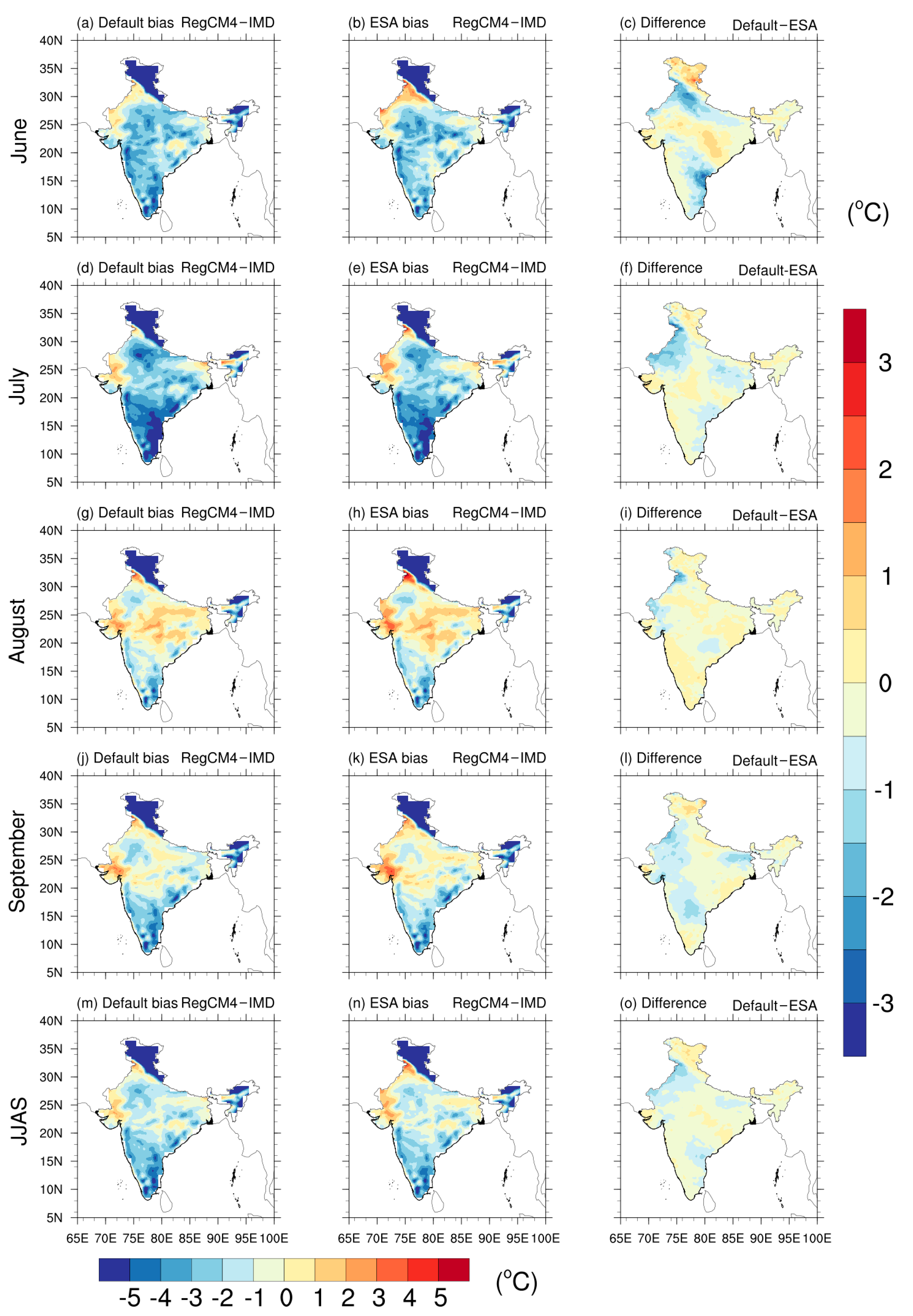
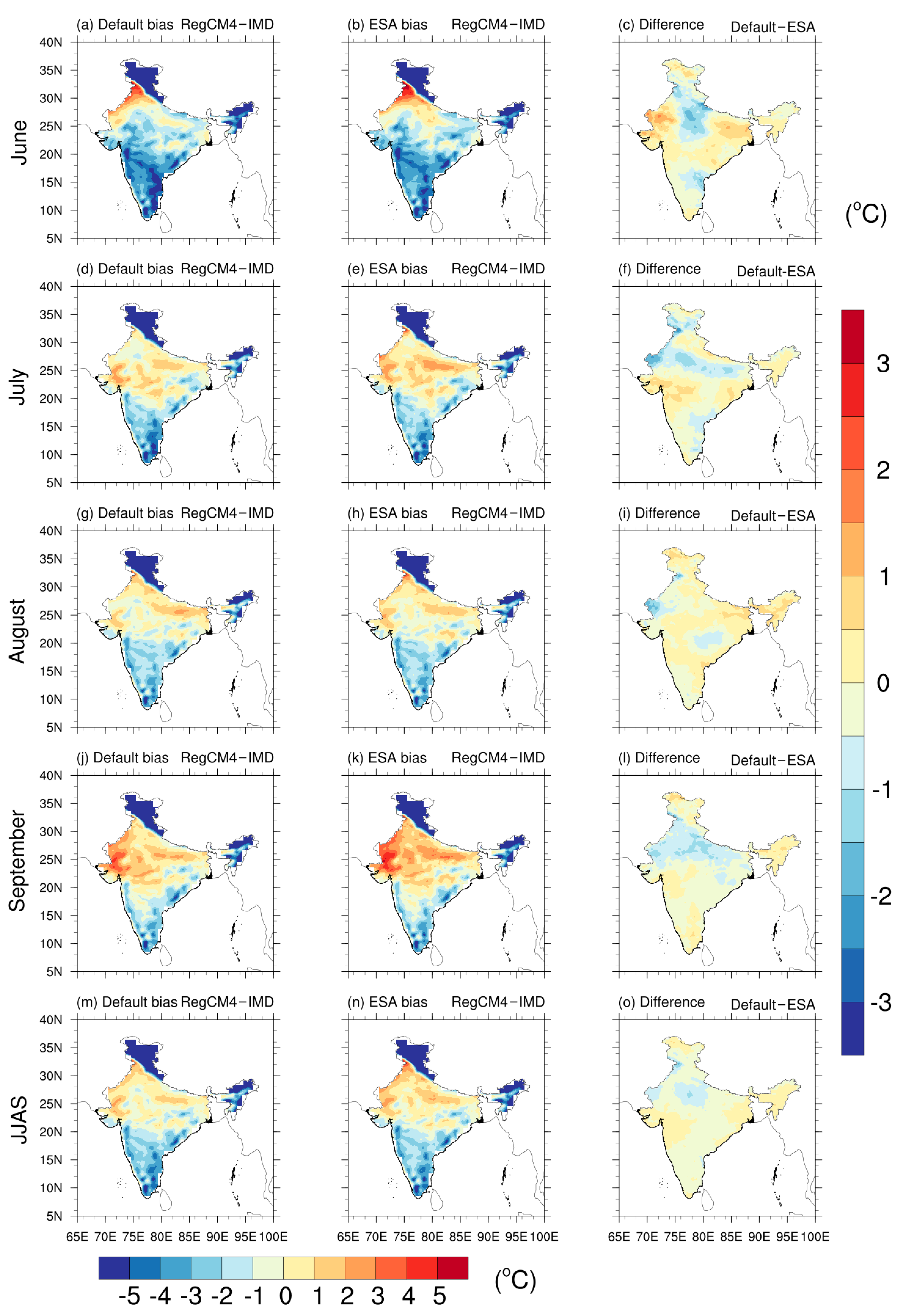
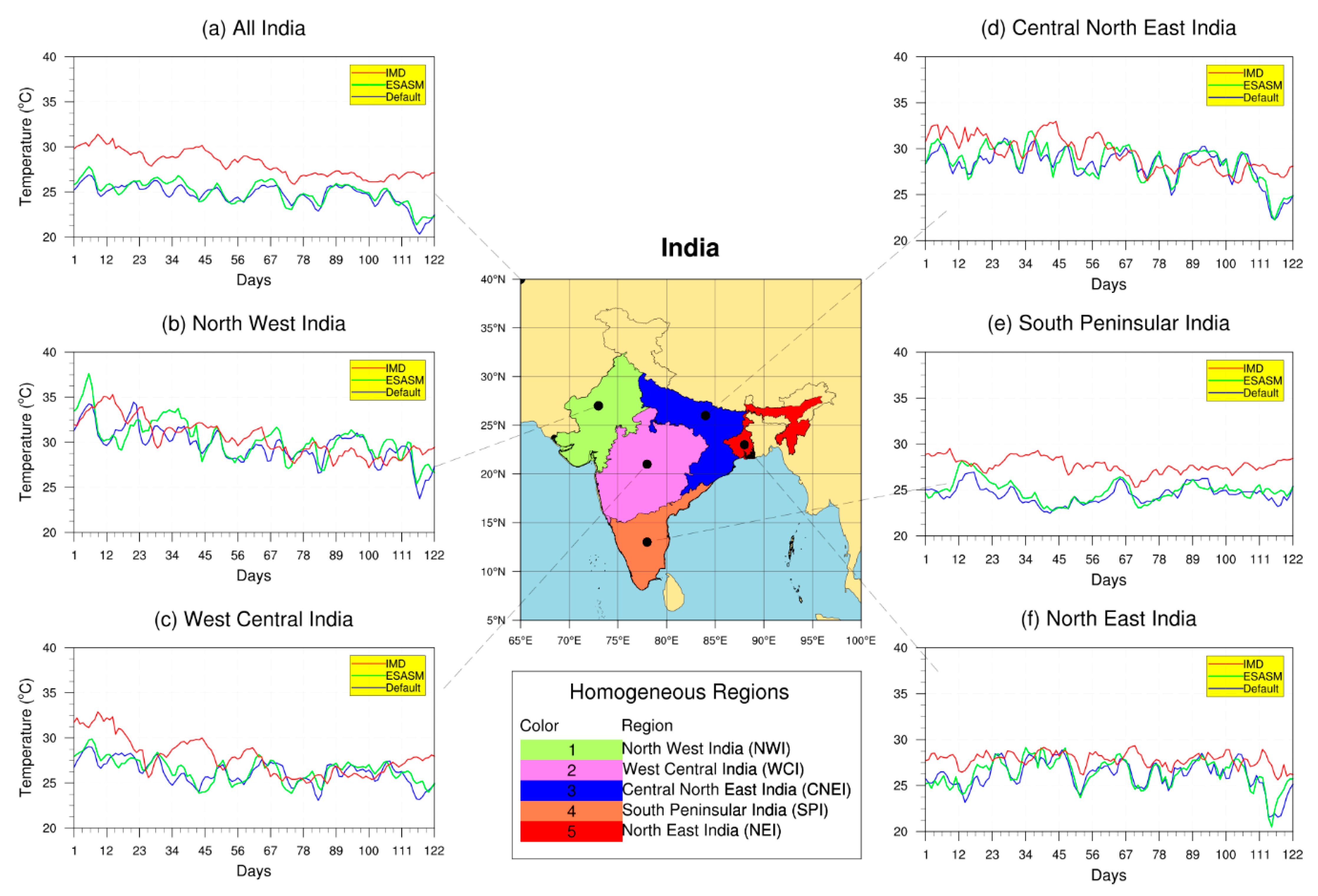
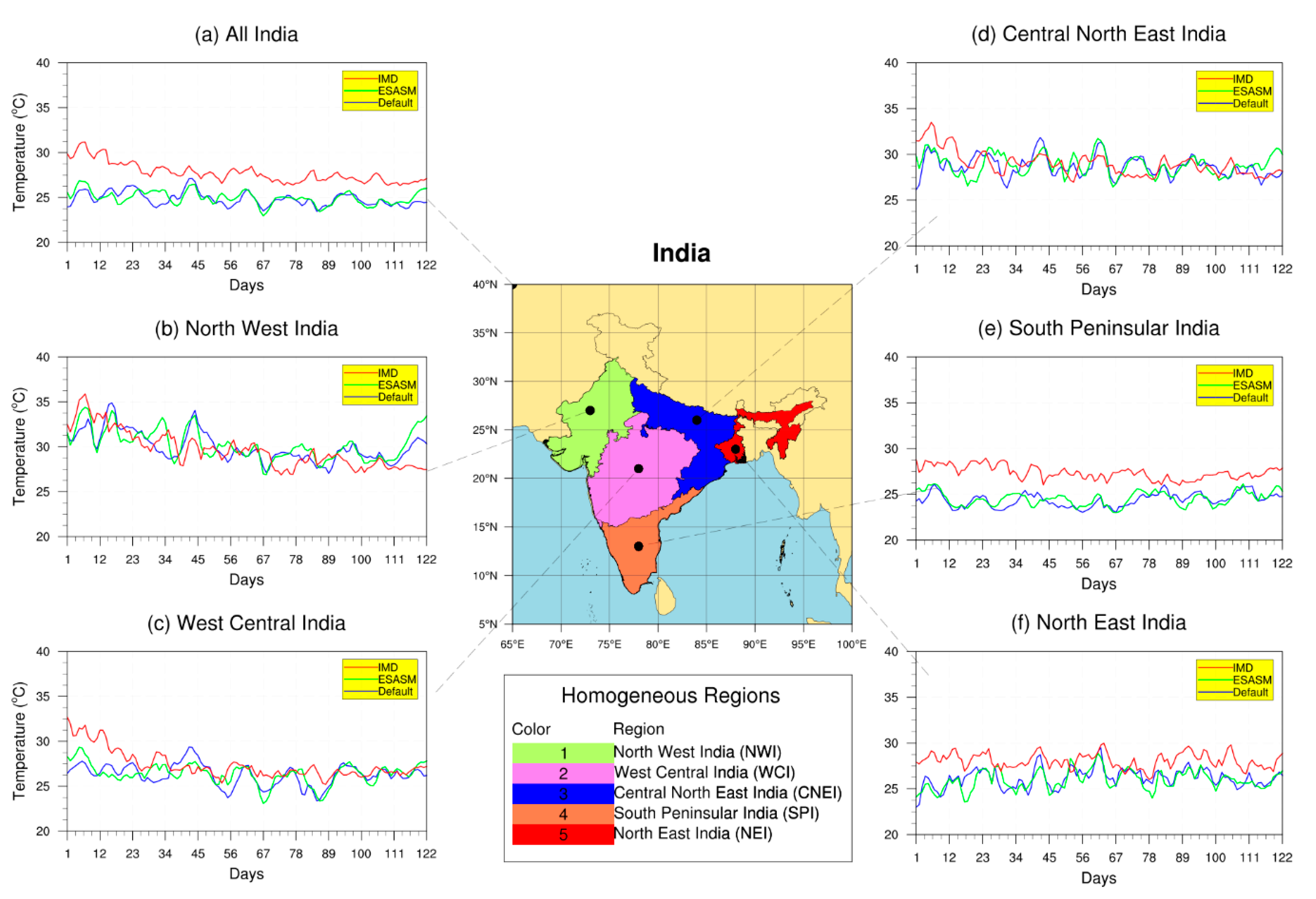
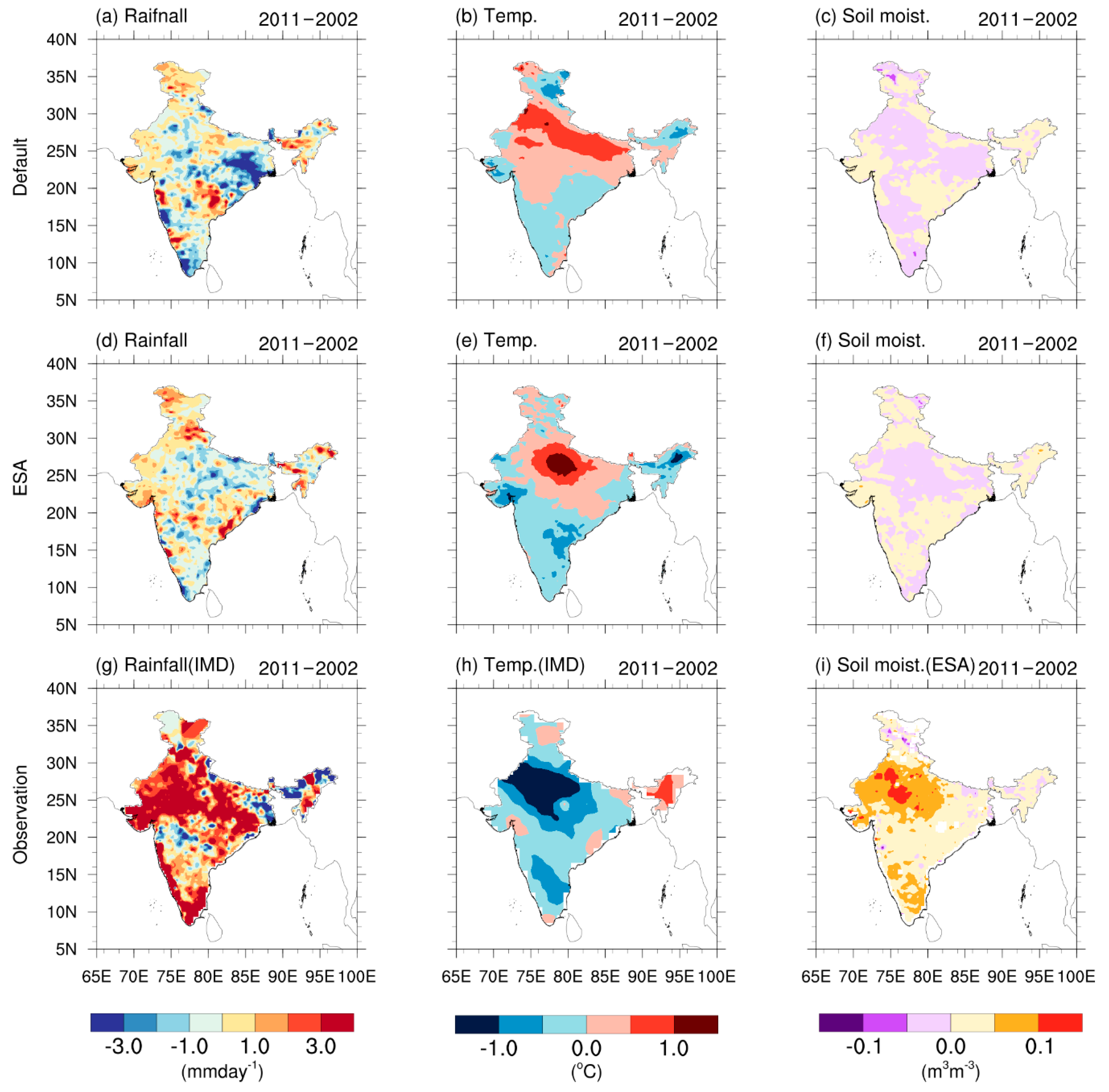
3.1. Surface Temperature
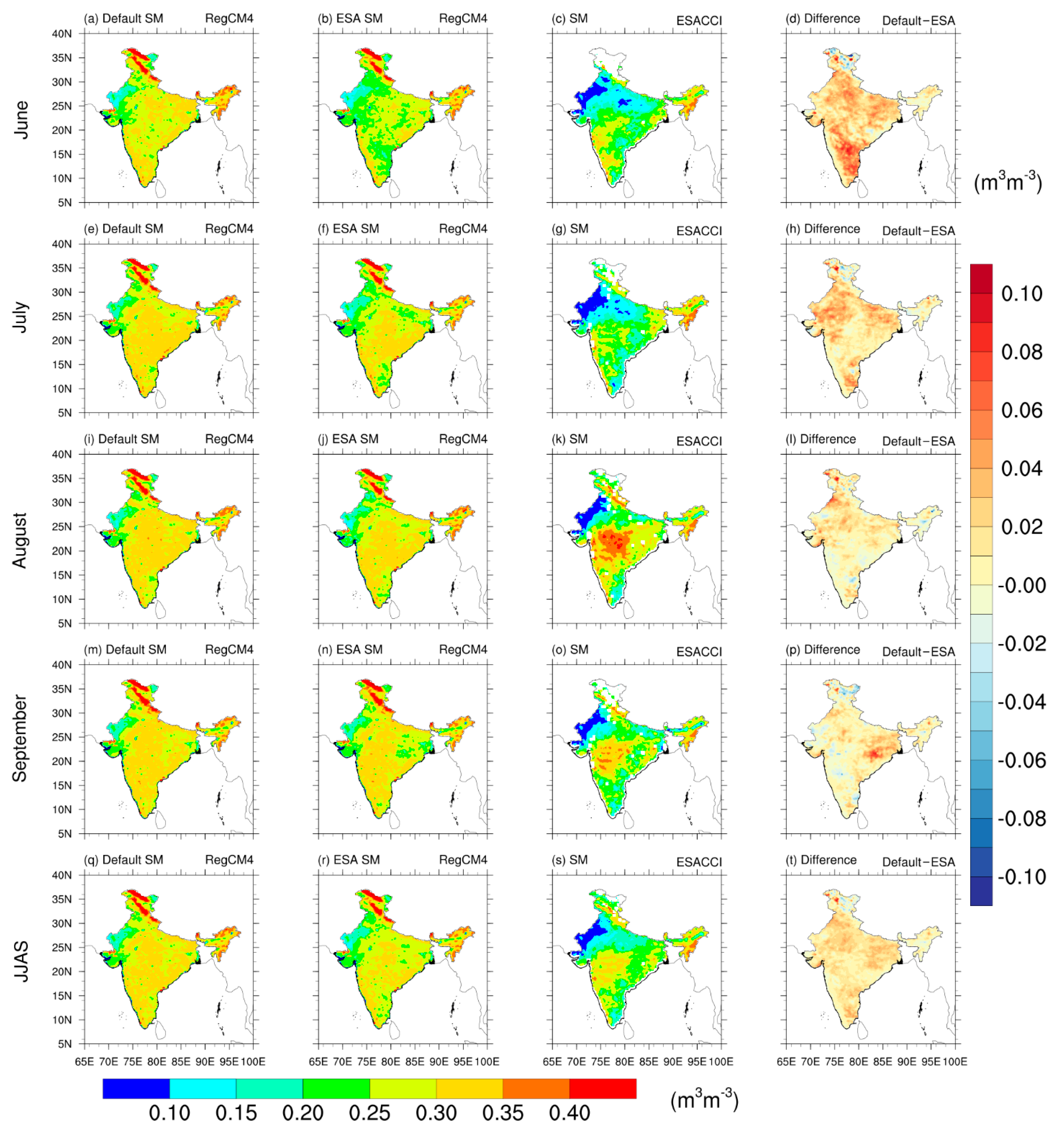
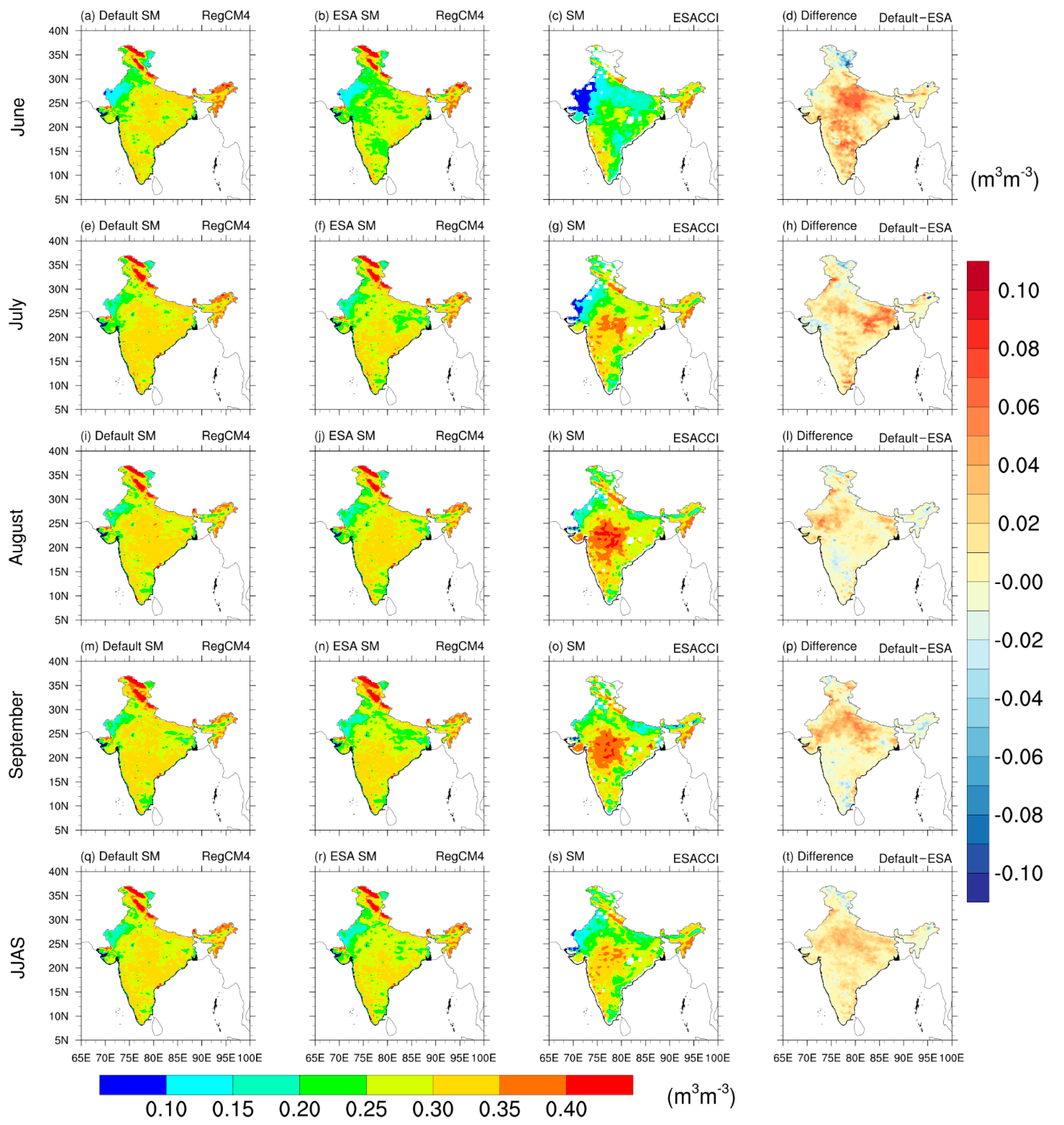
3.2. Soil Moisture
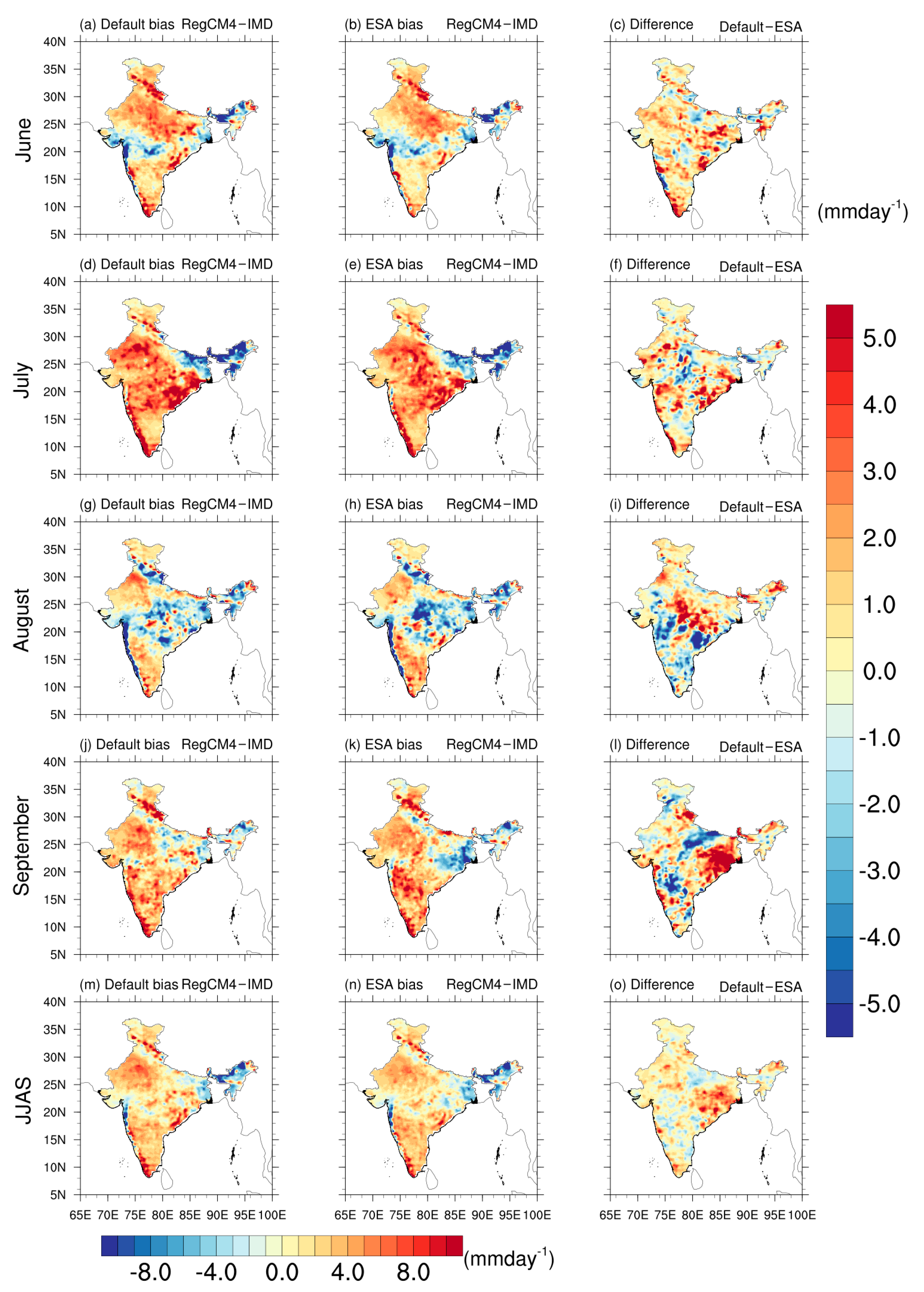
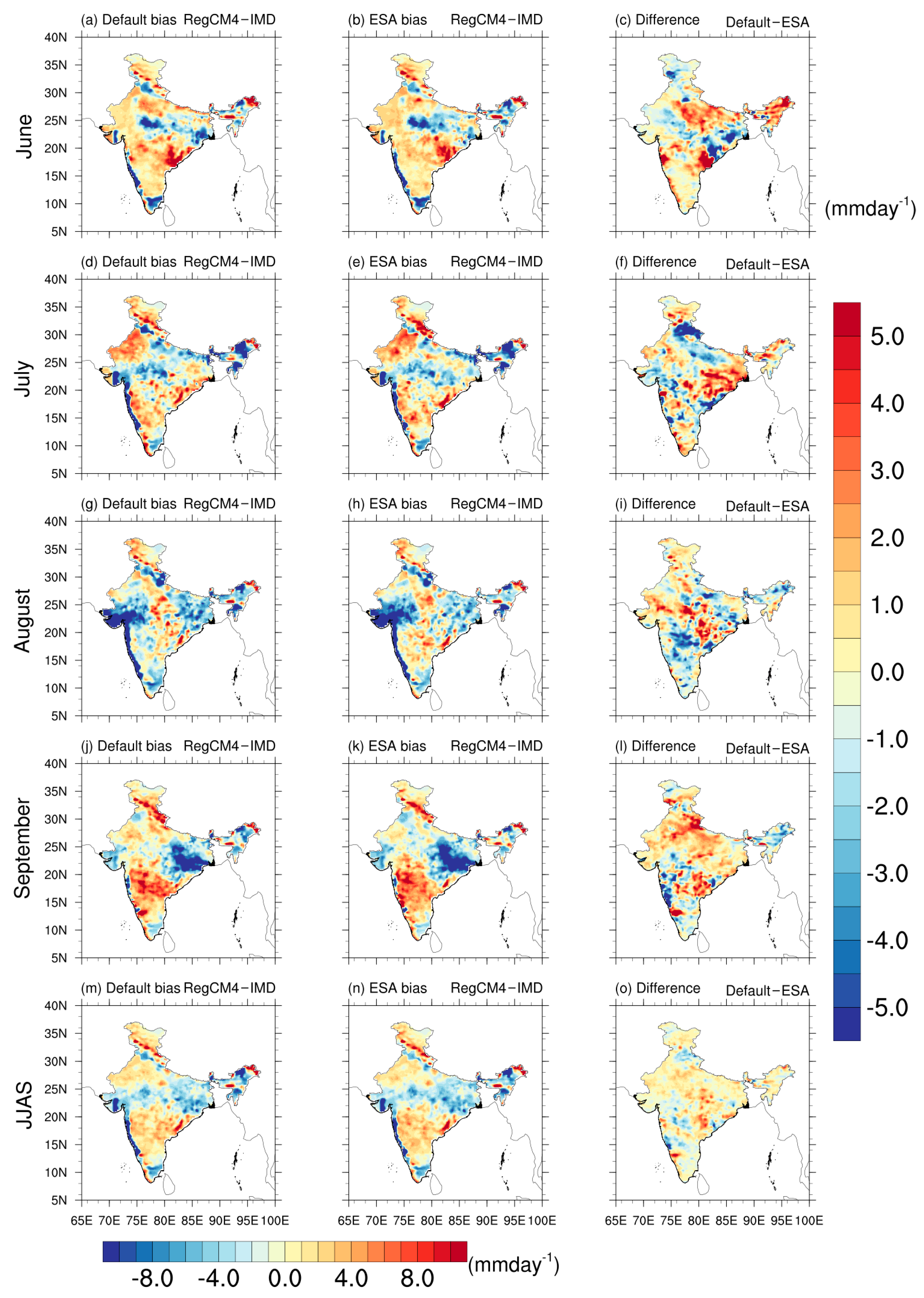
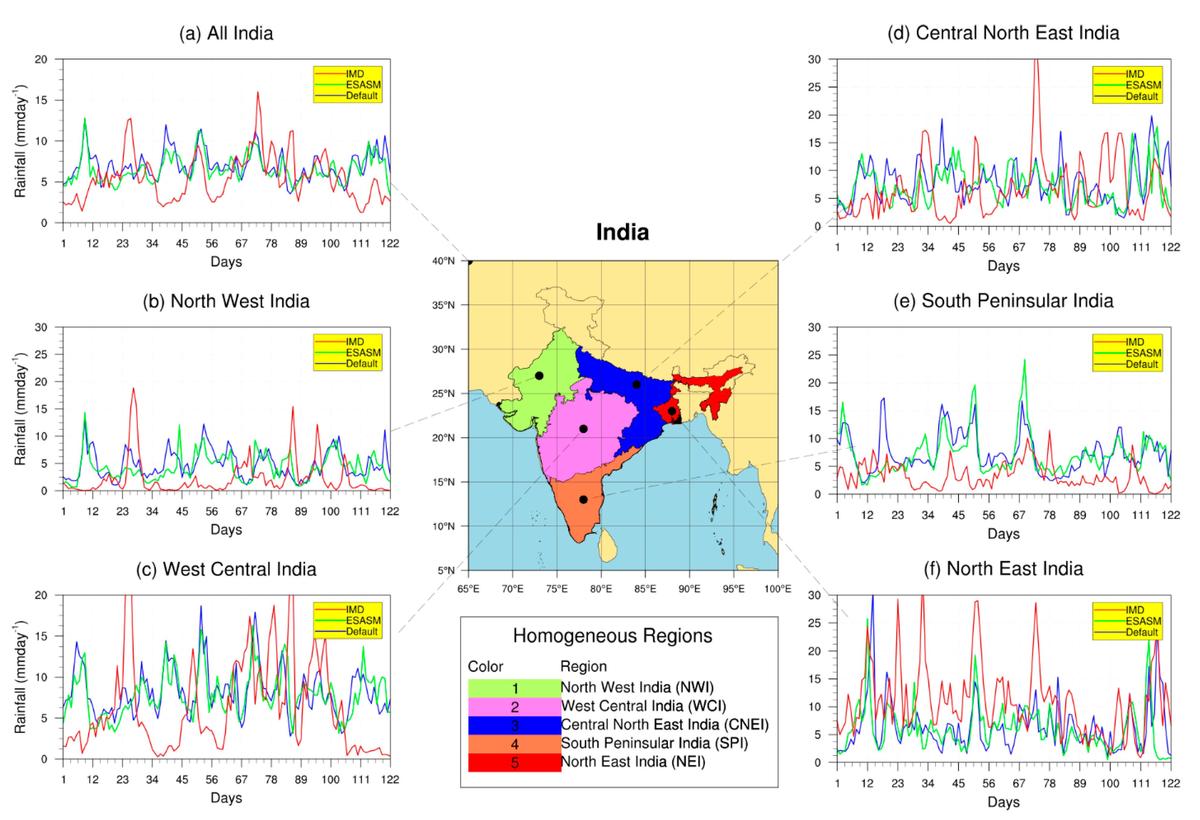
3.3. Rainfall
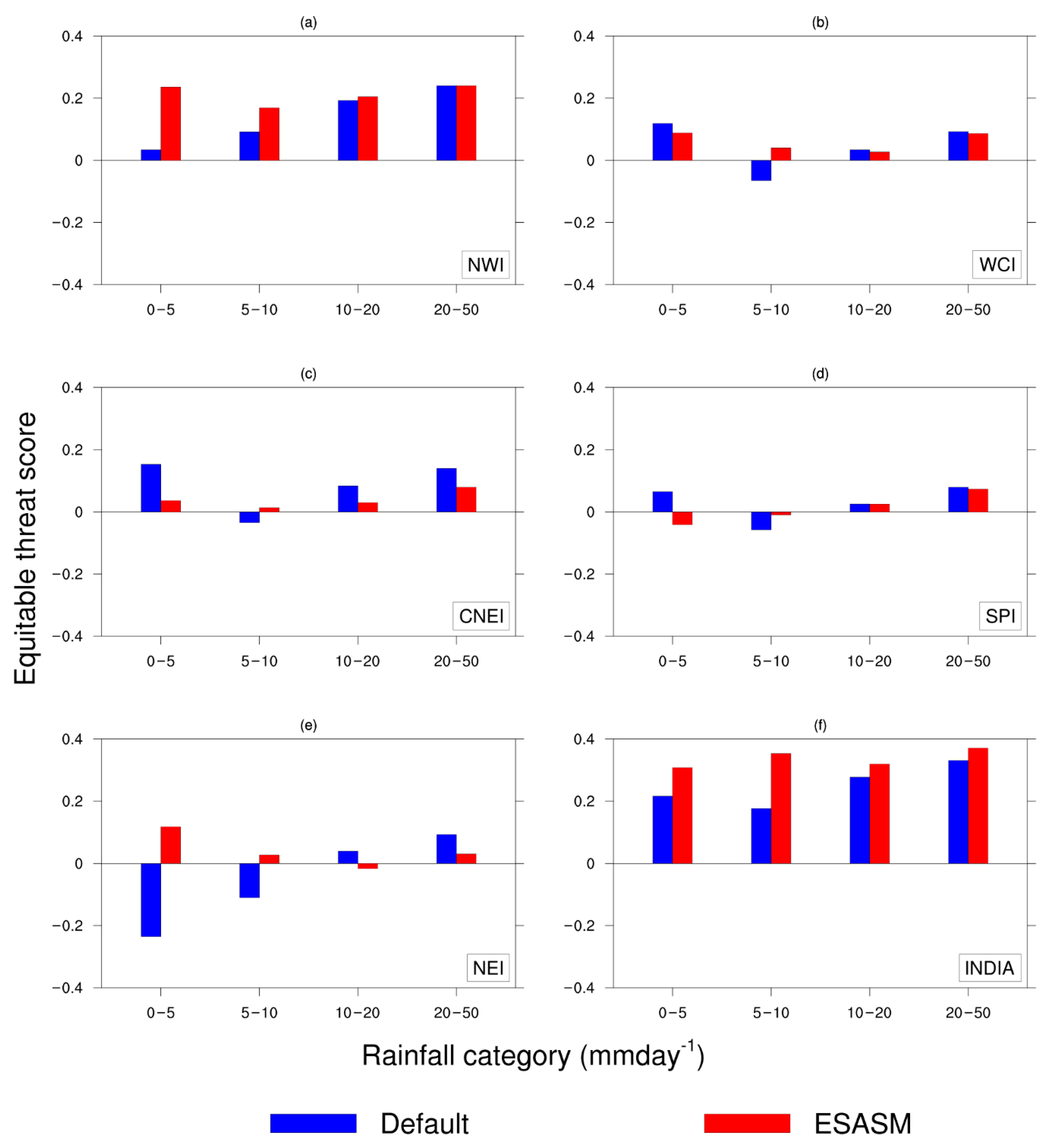
3.4. Quantitative Evaluation: Equitable Threat Score
4. Discussion
5. Conclusions
6. Limitation and Future Studies
Author Contributions
Funding
Institutional Review Board Statement
Informed Consent Statement
Data Availability Statement
Acknowledgments
Conflicts of Interest
References
- Steiner, A.L.; Pal, J.S.; Rauscher, S.A.; Bell, J.L.; Diffenbaugh, N.S.; Boone, A.; Sloan, L.C.; Giorgi, F. Land surface coupling in regional climate simulations of the West African monsoon. Clim. Dyn. 2009, 33, 869–892. [Google Scholar] [CrossRef]
- Moufouma-Okia, W.; Rowell, D.P. Impact of soil moisture initialisation and lateral boundary conditions on regional climate model simulations of the West African Monsoon. Clim. Dyn. 2010, 35, 213–229. [Google Scholar] [CrossRef]
- Douville, H. Relative contribution of soil moisture and snow mass to seasonal climate predictability: A pilot study. Clim. Dyn. 2010, 34, 797–818. [Google Scholar] [CrossRef]
- Bisselink, B.; Van Meijgaard, E.; Dolman, A.J.; De Jeu, R.A.M. Initializing a regional climate model with satellite-derived soil moisture. J. Geophys. Res. Atmos. 2011, 116. [Google Scholar] [CrossRef] [Green Version]
- Saha, S.K.; Halder, S.; Kumar, K.K.; Goswami, B.N. Pre-onset land surface processes and ‘internal’ interannual variabilities of the Indian summer monsoon. Clim. Dyn. 2011, 36, 2077–2089. [Google Scholar] [CrossRef]
- Van den Hurk, B.; Doblas-Reyes, F.; Balsamo, G.; Koster, R.D.; Seneviratne, S.I.; Camargo, H. Soil moisture effects on seasonal temperature and precipitation forecast scores in Europe. Clim. Dyn. 2012, 38, 349–362. [Google Scholar] [CrossRef] [Green Version]
- Suarez, A.; Mahmood, R.; Quintanar, A.I.; Beltran-Przekurat, A.; Pielke Sr, R. A comparison of the MM5 and the Regional Atmospheric Modeling System simulations for land–atmosphere interactions under varying soil moisture. Tellus A Dyn. Meteorol. Oceanogr. 2014, 66, 21486. [Google Scholar] [CrossRef]
- Chakravorty, A.; Chahar, B.R.; Sharma, O.P.; Dhanya, C.T. A regional scale performance evaluation of SMOS and ESA-CCI soil moisture products over India with simulated soil moisture from MERRA-Land. Remote Sens. Environ. 2016, 186, 514–527. [Google Scholar] [CrossRef]
- Lai, X.; Wen, J.; Cen, S.; Huang, X.; Tian, H.; Shi, X. Spatial and temporal soil moisture variations over China from simulations and observations. Adv. Meteorol. 2016, 2016, 4587687. [Google Scholar] [CrossRef] [Green Version]
- Sathyanadh, A.; Karipot, A.; Ranalkar, M.; Prabhakaran, T. Evaluation of soil moisture data products over Indian region and analysis of spatio-temporal characteristics with respect to monsoon rainfall. J. Hydrol. 2016, 542, 47–62. [Google Scholar] [CrossRef]
- Shrivastava, S.; Kar, S.C.; Sharma, A.R. Soil moisture variations in remotely sensed and reanalysis datasets during weak monsoon conditions over central India and central Myanmar. Theor. Appl. Climatol. 2017, 129, 305–320. [Google Scholar] [CrossRef]
- Nayak, S.; Maity, S.; Singh, K.S.; Nayak, H.P.; Dutta, S. Influence of the Changes in Land-Use and Land Cover on Temperature over Northern and North-Eastern India. Land 2021, 10, 52. [Google Scholar] [CrossRef]
- Nayak, S.; Mandal, M. Examining the impact of regional land use and land cover changes on temperature: The case of Eastern India. Spat. Inf. Res. 2019, 27, 601–611. [Google Scholar] [CrossRef]
- Nayak, S.; Mandal, M. Impact of land use and land cover changes on temperature trends over India. Land Use Policy 2019, 89, 1166–1173. [Google Scholar] [CrossRef]
- Giorgi, F.; Coppola, E.; Solmon, F.; Mariotti, L.; Sylla, M.B.; Bi, X.; Elguindi, N.; Diro, G.T.; Nair, V.; Giuliani, G.; et al. RegCM4: Model description and preliminary tests over multiple CORDEX domains. Clim. Res. 2012, 52, 7–29. [Google Scholar] [CrossRef] [Green Version]
- Dutta, S.K.; Das, S.; Kar, S.C.; Mohanty, U.C.; Joshi, P.C. Impact of downscaling on the simulation of seasonal monsoon rainfall over the Indian region using a global and mesoscale model. Open Atmos. Sci. J. 2009, 3, 104–123. [Google Scholar] [CrossRef] [Green Version]
- Maurya, R.K.S.; Sinha, P.; Mohanty, M.R.; Mohanty, U.C. Coupling of community land model with RegCM4 for Indian summer monsoon simulation. Pure Appl. Geophys. 2017, 174, 4251–4270. [Google Scholar] [CrossRef]
- Maity, S.; Mandal, M.; Nayak, S.; Bhatla, R. Performance of cumulus parameterization schemes in the simulation of Indian Summer Monsoon using RegCM4. Atmósfera 2017, 30, 287–309. [Google Scholar] [CrossRef] [Green Version]
- Maity, S.; Satyanarayana, A.N.V.; Mandal, M.; Nayak, S. Performance evaluation of land surface models and cumulus convection schemes in the simulation of Indian summer monsoon using a regional climate model. Atmos. Res. 2017, 197, 21–41. [Google Scholar] [CrossRef]
- Nayak, S.; Mandal, M.; Maity, S. Customization of regional climate model (RegCM4) over Indian region. Theor. Appl. Climatol. 2017, 127, 153–168. [Google Scholar] [CrossRef]
- Nayak, S.; Mandal, M.; Maity, S. RegCM4 simulation with AVHRR land use data towards temperature and precipitation climatology over Indian region. Atmos. Res. 2018, 214, 163–173. [Google Scholar] [CrossRef]
- Nayak, S.; Mandal, M.; Maity, S. Performance evaluation of RegCM4 in simulating temperature and precipitation climatology over India. Theor. Appl. Climatol. 2019, 137, 1059–1075. [Google Scholar] [CrossRef]
- Leng, G.; Huang, M.; Tang, Q.; Sacks, W.J.; Lei, H.; Leung, L.R. Modeling the effects of irrigation on land surface fluxes and states over the conterminous United States: Sensitivity to input data and model parameters. J. Geophys. Res. Atmos. 2013, 118, 9789–9803. [Google Scholar] [CrossRef]
- Fennessy, M.J.; Shukla, J. Impact of initial soil wetness on seasonal atmospheric prediction. J. Clim. 1999, 12, 3167–3180. [Google Scholar] [CrossRef]
- Douville, H.; Chauvin, F. Relevance of soil moisture for seasonal climate predictions: A preliminary study. Clim. Dyn. 2000, 16, 719–736. [Google Scholar] [CrossRef]
- Pan, Z.; Arritt, R.W.; Gutowski, W.J., Jr.; Takle, E.S. Soil moisture in a regional climate model: Simulation and projection. Geophys. Res. Lett. 2001, 28, 2947–2950. [Google Scholar] [CrossRef] [Green Version]
- Kanamitsu, M.; Lu, C.H.; Schemm, J.; Ebisuzaki, W. The predictability of soil moisture and near-surface temperature in hindcasts of the NCEP seasonal forecast model. J. Clim. 2003, 16, 510–521. [Google Scholar] [CrossRef]
- Douville, H. Relevance of soil moisture for seasonal atmospheric predictions: Is it an initial value problem? Clim. Dyn. 2004, 22, 429–446. [Google Scholar] [CrossRef]
- Tawfik, A.B.; Steiner, A.L. The role of soil ice in land-atmosphere coupling over the United States: A soil moisture–precipitation winter feedback mechanism. J. Geophys. Res. Atmos. 2011, 116. [Google Scholar] [CrossRef] [Green Version]
- Patarcic, M.; Brankovic, C. Skill of 2-m temperature seasonal forecasts over Europe in ECMWF and RegCM models. Mon. Weather Rev. 2012, 140, 1326–1346. [Google Scholar] [CrossRef]
- Liu, D.; Wang, G.; Mei, R.; Yu, Z.; Yu, M. Impact of initial soil moisture anomalies on climate mean and extremes over Asia. J. Geophys. Res. Atmos. 2014, 119, 529–545. [Google Scholar] [CrossRef]
- Nayak, H.P.; Osuri, K.K.; Sinha, P.; Nadimpalli, R.; Mohanty, U.C.; Chen, F.; Rajeevan, M.; Niyogi, D. High-resolution gridded soil moisture and soil temperature datasets for the Indian monsoon region. Sci. Data 2018, 5, 1–17. [Google Scholar] [CrossRef] [PubMed]
- Nayak, H.P.; Sinha, P.; Mohanty, U.C. Incorporation of surface observations in the LDAS and application to mesoscale simulation of pre-monsoon thunderstorms. Pure Appl. Geophys. 2021, 178, 565–582. [Google Scholar] [CrossRef]
- Gianotti, R.L.; Zhang, D.; Eltahir, E.A. Assessment of the regional climate model version 3 over the maritime continent using different cumulus parameterization and land surface schemes. J. Clim. 2012, 25, 638–656. [Google Scholar] [CrossRef]
- Llopart, M.; da Rocha, R.P.; Reboita, M.; Cuadra, S. Sensitivity of simulated South America climate to the land surface schemes in RegCM4. Clim. Dyn. 2017, 49, 3975–3987. [Google Scholar] [CrossRef] [Green Version]
- Nayak, S.; Mandal, M.; Maity, S. Assessing the impact of Land-use and Land-cover changes on the climate over India using a Regional Climate Model (RegCM4). Clim. Res. 2021, in press. [Google Scholar] [CrossRef]
- Bhatla, R.; Ghosh, S.; Mandal, B.; Mall, R.K.; Sharma, K. Simulation of Indian summer monsoon onset with different parameterization convection schemes of RegCM-4.3. Atmos. Res. 2016, 176, 10–18. [Google Scholar] [CrossRef]
- Hu, Y.; Ding, Y.; Liao, F. An improvement on summer regional climate simulation over East China: Importance of data assimilation of soil moisture. Chin. Sci. Bull. 2010, 55, 865–871. [Google Scholar] [CrossRef]
- Parinussa, R.M.; Yilmaz, M.T.; Anderson, M.C.; Hain, C.R.; De Jeu, R.A.M. An intercomparison of remotely sensed soil moisture products at various spatial scales over the Iberian Peninsula. Hydrol. Process. 2014, 28, 4865–4876. [Google Scholar] [CrossRef]
- Pieczka, I.; Pongrácz, R.; André, K.S.; Kelemen, F.D.; Bartholy, J. Sensitivity analysis of different parameterization schemes using RegCM4.3 for the Carpathian region. Theor. Appl. Climatol. 2017, 130, 1175–1188. [Google Scholar] [CrossRef]
- Pal, J.S.; Giorgi, F.; Bi, X.; Elguindi, N.; Solmon, F.; Gao, X.; Rauscher, S.A.; Francisco, R.; Zakey, A.; Winter, J.; et al. Regional climate modeling for the developing world: The ICTP RegCM3 and RegCNET. Bull. Am. Meteorol. Soc. 2007, 88, 1395–1410. [Google Scholar] [CrossRef] [Green Version]
- Anthes, R.A. A cumulus parameterization scheme utilizing a one-dimensional cloud model. Mon. Weather Rev. 1977, 105, 270–286. [Google Scholar] [CrossRef] [Green Version]
- Grell, G.A. Prognostic evaluation of assumptions used by cumulus parameterizations. Mon. Weather Rev. 1993, 121, 764–787. [Google Scholar] [CrossRef] [Green Version]
- Emanuel, K.A. A scheme for representing cumulus convection in large-scale models. J. Atmos. Sc. 1991, 48, 2313–2329. [Google Scholar] [CrossRef]
- Tiedtke, M.I.C.H.A.E.L. A comprehensive mass flux scheme for cumulus parameterization in large-scale models. Mon. Weather Rev. 1989, 117, 1779–1800. [Google Scholar] [CrossRef] [Green Version]
- Kain, J.S.; Fritsch, J.M. Convective parameterization for mesoscale models: The Kain-Fritsch scheme. In The representation of cumulus convection in numerical models. Meteorological Monographs. Am. Meteor. Soc. 1993, 165–170. [Google Scholar] [CrossRef]
- Dickinson, R.E.; Errico, R.M.; Giorgi, F.; Bates, G.T.; Henderson-Sellers, A.; Kennedy, P.J. Biosphere–Atmosphere Transfer Scheme (BATS) Version 1e as Coupled to the NCAR Community Climate Model; NCAR Tech. Note NCAR/TN-3871STR; National Center for Atmospheric Research: Boulder, CO, USA, 1993.
- Oleson, K.W.; Niu, G.Y.; Yang, Z.L.; Lawrence, D.M.; Thornton, P.E.; Lawrence, P.J.; Stöckli, R.; Dickinson, R.E.; Bonan, G.B.; Levis, S.; et al. Improvements to the Community Land Model and their impact on the hydrological cycle. J. Geophys. Res. Biogeosci. 2008, 113. [Google Scholar] [CrossRef]
- Bonan, G.; Drewniak, B.; Huang, M. Technical Description of Version 4.5 of the Community Land Model (CLM); NCAR Technical Note NCAR/TN-503+ STR; National Center for Atmospheric Research: Boulder, CO, USA, 2013.
- Kiehl, T.; Hack, J.; Bonan, B.; Boville, A.; Briegleb, P.; Williamson, L.; Rasch, J. Description of the NCAR Community Climate Model (CCM3); Technical Note (No. PB-97-131528/XAB.; NCAR/TN-420-STR); National Center for Atmospheric Research: Boulder, CO, USA, 1996.
- Holtslag, A.A.M.; De Bruijn, E.I.F.; Pan, H.L. A high resolution air mass transformation model for short-range weather forecasting. Mon. Weather Rev. 1990, 118, 1561–1575. [Google Scholar] [CrossRef]
- Bretherton, C.S.; McCaa, J.R.; Grenier, H. A new parameterization for shallow cumulus convection and its application to marine subtropical cloud-topped boundary layers. Part I: Description and 1D results. Mon. Weather Rev. 2004, 132, 864–882. [Google Scholar] [CrossRef] [Green Version]
- Halder, S.; Dirmeyer, P.A.; Saha, S.K. Sensitivity of the mean and variability of Indian summer monsoon to land surface schemes in RegCM4: Understanding coupled land-atmosphere feedbacks. J. Geophys. Res. Atmos. 2015, 120, 9437–9458. [Google Scholar] [CrossRef] [Green Version]
- Giorgi, F.; Bates, G.T. The climatological skill of a regional model over complex terrain. Mon. Weather Rev. 1989, 117, 2325–2347. [Google Scholar] [CrossRef] [Green Version]
- Steiner, A.L.; Pal, J.S.; Giorgi, F.; Dickinson, R.E.; Chameides, W.L. The coupling of the Common Land Model (CLM0) to a regional climate model (RegCM). Theor. Appl. Climatol. 2005, 82, 225–243. [Google Scholar] [CrossRef]
- Chaudhari, H.S.; Shinde, M.A.; Oh, J.H. Understanding of anomalous Indian summer monsoon rainfall of 2002 and 1994. Quat. Int. 2010, 213, 20–32. [Google Scholar] [CrossRef]
- Maity, S. Comparative assessment of two RegCM versions in simulating Indian Summer Monsoon. J. Earth Syst. Sci. 2020, 129, 1–23. [Google Scholar] [CrossRef]
- Arakawa, A.; Schubert, W.H. Interaction of a cumulus cloud ensemble with the large-scale environment, Part I. J. Atmos. Sci. 1974, 31, 674–701. [Google Scholar] [CrossRef] [Green Version]
- Pal, J.S.; Small, E.E.; Eltahir, E.A. Simulation of regional-scale water and energy budgets: Representation of subgrid cloud and precipitation processes within RegCM. J. Geophys. Res. Atmos. 2000, 105, 29579–29594. [Google Scholar] [CrossRef] [Green Version]
- Zeng, X.; Zhao, M.; Dickinson, R.E. Intercomparison of bulk aerodynamic algorithms for the computation of sea surface fluxes using TOGA COARE and TAO data. J. Clim. 1998, 11, 2628–2644. [Google Scholar] [CrossRef]
- Dorigo, W.; Wagner, W.; Albergel, C.; Albrecht, F.; Balsamo, G.; Brocca, L.; Chung, D.; Ertl, M.; Forkel, M.; Gruber, A.; et al. ESA CCI Soil Moisture for improved Earth system understanding: State-of-the art and future directions. Remote Sens. Environ. 2017, 203, 185–215. [Google Scholar] [CrossRef]
- Dorigo, W.A.; Gruber, A.; De Jeu, R.A.M.; Wagner, W.; Stacke, T.; Loew, A.; Albergel, C.; Brocca, L.; Chung, D.; Parinussa, R.M.; et al. Evaluation of the ESA CCI soil moisture product using ground-based observations. Remote Sens. Environ. 2015, 162, 380–395. [Google Scholar] [CrossRef]
- Dee, D.P.; Uppala, S.M.; Simmons, A.J.; Berrisford, P.; Poli, P.; Kobayashi, S.; Andrae, U.; Balmaseda, M.A.; Balsamo, G.; Bauer, D.P.; et al. The ERA-Interim reanalysis: Configuration and performance of the data assimilation system. Q. J. R. Meteorol. Soc. 2011, 137, 553–597. [Google Scholar] [CrossRef]
- Loveland, T.R.; Reed, B.C.; Brown, J.F.; Ohlen, D.O.; Zhu, Z.; Yang, L.W.M.J.; Merchant, J.W. Development of a global land cover characteristics database and IGBP DISC over from 1 km AVHRR data. Int. J. Remote Sens. 2000, 21, 1303–1330. [Google Scholar] [CrossRef]
- Reynolds, R.W.; Rayner, N.A.; Smith, T.M.; Stokes, D.C.; Wang, W. An improved in situ and satellite SST analysis for climate. J. Clim. 2002, 15, 1609–1625. [Google Scholar] [CrossRef]
- Srivastava, A.K.; Rajeevan, M.; Kshirsagar, S.R. Development of a high resolution daily gridded temperature data set (1969–2005) for the Indian region. Atmos. Sci. Lett. 2009, 10, 249–254. [Google Scholar] [CrossRef]
- Pai, D.S.; Sridhar, L.; Rajeevan, M.; Sreejith, O.P.; Satbhai, N.S.; Mukhopadhyay, B. Development of a new high spatial resolution (0.25 × 0.25) long period (1901–2010) daily gridded rainfall data set over India and its comparison with existing data sets over the region. Mausam 2014, 65, 1–18. [Google Scholar]
- Liu, Y.Y.; Parinussa, R.M.; Dorigo, W.A.; De Jeu, R.A.; Wagner, W.; Van Dijk, A.I.J.M.; McCabe, M.F.; Evans, J.P. Developing an improved soil moisture dataset by blending passive and active microwave satellite-based retrievals. Hydrol. Earth Syst. Sci. 2011, 15, 425–436. [Google Scholar] [CrossRef] [Green Version]
- Parthasarathy, B.; Munot, A.A.; Kothawale, D.R. All-India monthly and seasonal rainfall series: 1871–1993. Theor. Appl. Climatol. 1994, 49, 217–224. [Google Scholar] [CrossRef]
- Mesinger, F. Improvements in quantitative precipitation forecasts with the Eta regional model at the National Centers for Environmental Prediction: The 48-km upgrade. Bull. Am. Meteorol. Soc. 1996, 77, 2637–2650. [Google Scholar] [CrossRef] [Green Version]
- Gilbert, G.K. Finley’s tornado predictions. Am. Meteorol. J. 1884, 1, 166. [Google Scholar]
- Zhang, H.; Liu, J.; Li, H.; Meng, X.; Ablikim, A. The Impacts of Soil Moisture Initialization on the Forecasts of Weather Research and Forecasting Model: A Case Study in Xinjiang, China. Water 2020, 12, 1892. [Google Scholar] [CrossRef]


| Contents | Description |
|---|---|
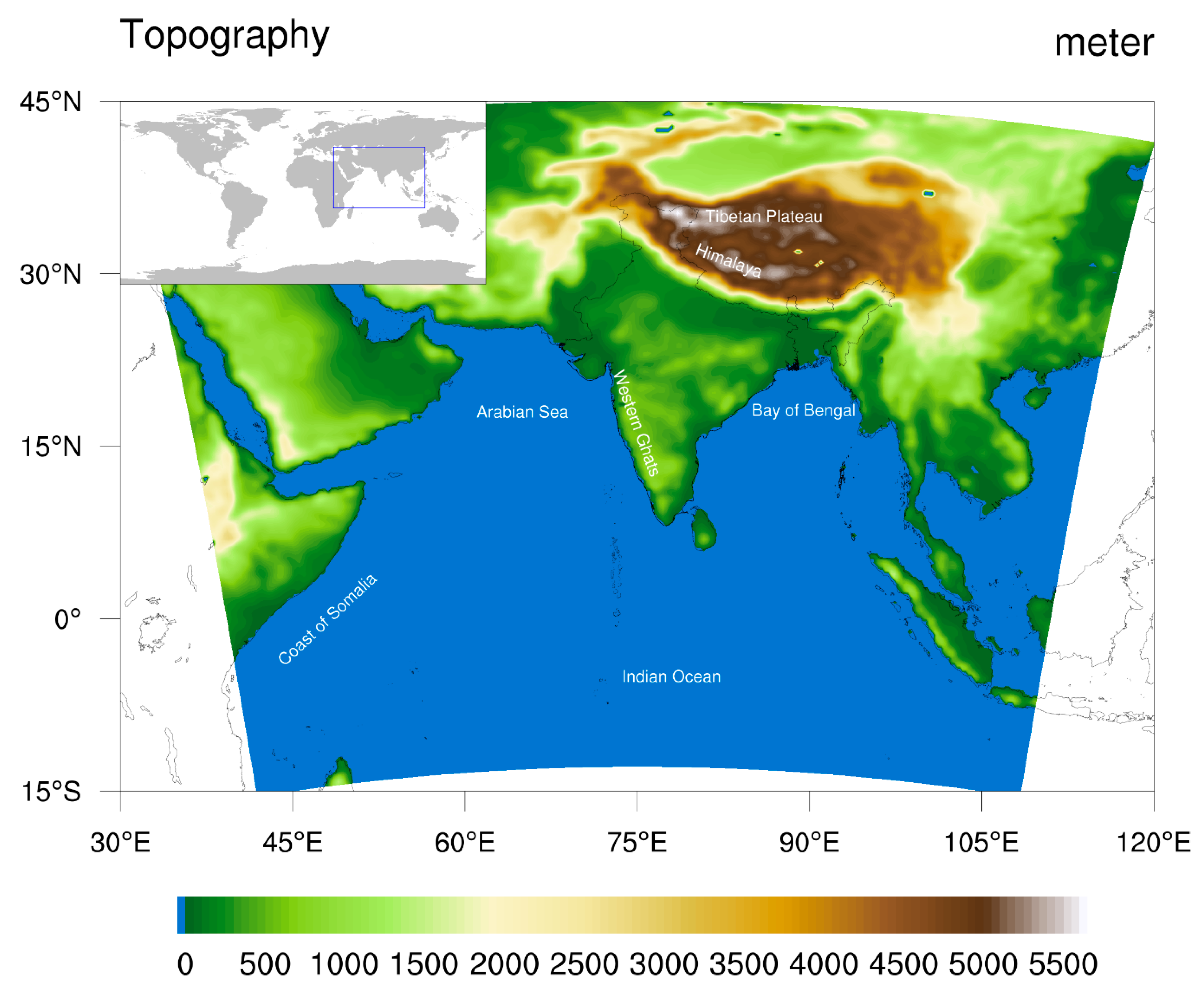
| Model domain | South Asia (30° E–120° E; 15° S–45° N) |
| Resolution | Horizontal: 30 km, vertical: 23 terrain following levels |
| Land surface | CLM4.5 [49] |
| Cumulus convection | Grell [43] over ocean and MIT [44] over land |
| Cumulus closure | Arakawa and Schubert [58] |
| Explicit moisture | SUBEX [59] |
| Ocean flux | Zeng [60] |
| 2002 | 2011 | |||||||||
|---|---|---|---|---|---|---|---|---|---|---|
| Correlation | Standard Deviation | Correlation | Standard Deviation | |||||||
| Default | ESASM | Default | ESASM | IMD | Default | ESASM | Default | ESASM | IMD | |
| NWI | 0.52 * | 0.48 * | 1.95 | 2.20 | 2.03 | 0.59 * | 0.54 * | 1.66 | 1.72 | 2.05 |
| WCI | 0.34 * | 0.39 * | 1.33 | 1.34 | 2.09 | 0.31 * | 0.50 * | 1.20 | 1.16 | 1.56 |
| CNEI | 0.42 * | 0.43 * | 1.84 | 1.94 | 1.81 | 0.32 * | 0.28 * | 1.33 | 1.17 | 1.33 |
| SPI | −0.13 † | 0.03 † | 0.98 | 1.15 | 0.83 | −0.10 † | 0.04 † | 0.75 | 0.78 | 0.74 |
| NEI | 0.46 * | 0.41 * | 1.62 | 1.58 | 0.78 | 0.38 * | 0.39 * | 1.06 | 1.06 | 0.83 |
| INDIA | 0.46 * | 0.49 * | 1.24 | 1.28 | 1.43 | 0.44 * | 0.47 * | 0.77 | 0.77 | 1.11 |
| 2002 | 2011 | |||||||||
|---|---|---|---|---|---|---|---|---|---|---|
| Correlation | Standard Deviation | Correlation | Standard Deviation | |||||||
| Default | ESASM | Default | ESASM | IMD | Default | ESASM | Default | ESASM | IMD | |
| NWI | −0.14 † | −0.14 † | 2.62 | 2.48 | 3.37 | 0.27 * | 0.38 * | 2.80 | 2.80 | 5.56 |
| WCI | −0.14 † | −0.12 † | 2.98 | 2.81 | 5.89 | 0.16 † | 0.22 * | 2.63 | 2.66 | 4.81 |
| CNEI | −0.06 † | −0.03 † | 3.77 | 3.29 | 5.62 | 0.41 * | 0.19 * | 2.83 | 3.29 | 5.29 |
| SPI | −0.07 † | −0.03 † | 3.52 | 3.77 | 2.24 | 0.02 † | 0.03 † | 3.39 | 3.69 | 5.11 |
| NEI | 0.40 * | 0.34 * | 4.67 | 4.12 | 6.41 | 0.11 † | 0.17 † | 3.74 | 3.43 | 5.49 |
| INDIA | −0.04 † | 0.03 † | 1.77 | 1.70 | 2.86 | 0.51 * | 0.47 * | 1.43 | 1.64 | 2.99 |
Publisher’s Note: MDPI stays neutral with regard to jurisdictional claims in published maps and institutional affiliations. |
© 2021 by the authors. Licensee MDPI, Basel, Switzerland. This article is an open access article distributed under the terms and conditions of the Creative Commons Attribution (CC BY) license (https://creativecommons.org/licenses/by/4.0/).
Share and Cite
Maity, S.; Nayak, S.; Singh, K.S.; Nayak, H.P.; Dutta, S. Impact of Soil Moisture Initialization in the Simulation of Indian Summer Monsoon Using RegCM4. Atmosphere 2021, 12, 1148. https://doi.org/10.3390/atmos12091148
Maity S, Nayak S, Singh KS, Nayak HP, Dutta S. Impact of Soil Moisture Initialization in the Simulation of Indian Summer Monsoon Using RegCM4. Atmosphere. 2021; 12(9):1148. https://doi.org/10.3390/atmos12091148
Chicago/Turabian StyleMaity, Suman, Sridhara Nayak, Kuvar Satya Singh, Hara Prasad Nayak, and Soma Dutta. 2021. "Impact of Soil Moisture Initialization in the Simulation of Indian Summer Monsoon Using RegCM4" Atmosphere 12, no. 9: 1148. https://doi.org/10.3390/atmos12091148