Article

Future Projections and Uncertainty Assessment of Precipitation Extremes in Iran from the CMIP6 Ensemble

1
Department of Mathematics and Statistics, Chonnam National University, Gwangju 61186, Korea
2
Department of Geography, Urmia University, Urmia 009844, Iran
*
Author to whom correspondence should be addressed.
Atmosphere 2021, 12(8), 1052; https://doi.org/10.3390/atmos12081052
Submission received: 8 July 2021 / Revised: 11 August 2021 / Accepted: 11 August 2021 / Published: 16 August 2021

Abstract

:
Scientists who want to know future climate can use multimodel ensemble (MME) methods that combine projections from individual simulation models. To predict the future changes of extreme rainfall in Iran, we examined the observations and 24 models of the Coupled Model Inter-Comparison Project Phase 6 (CMIP6) over the Middle East. We applied generalized extreme value (GEV) distribution to series of annual maximum daily precipitation (AMP1) data obtained from both of models and the observations. We also employed multivariate bias-correction under three shared socioeconomic pathway (SSP) scenarios (namely, SSP2-4.5, SSP3-7.0, and SSP5-8.5). We used a model averaging method that takes both performance and independence of model into account, which is called PI-weighting. Return levels for 20 and 50 years, as well as the return periods of the AMP1 relative to the reference years (1971–2014), were estimated for three future periods. These are period 1 (2021–2050), period 2 (2046–2075), and period 3 (2071–2100). From this study, we predict that over Iran the relative increases of 20-year return level of the AMP1 in the spatial median from the past observations to the year 2100 will be approximately 15.6% in the SSP2-4.5, 23.2% in the SSP3-7.0, and 28.7% in the SSP5-8.5 scenarios, respectively. We also realized that a 1-in-20 year (or 1-in-50 year) AMP1 observed in the reference years in Iran will likely become a 1-in-12 (1-in-26) year, a 1-in-10 (1-in-22) year, and a 1-in-9 (1-in-20) year event by 2100 under the SSP2-4.5, SSP3-7.0, and SSP5-8.5 scenarios, respectively. We project that heavy rainfall will be more prominent in the western and southwestern parts of Iran.

1. Introduction

Extreme rain events can result in landslides and floods, accompanied with a loss of life and the deterioration of infrastructure. Thus, understanding and projecting heavy rainfall is of significant importance to climate change impact, adaptation, and vulnerability assessments.
Numerous studies have reported that extreme precipitation events have become more frequent during the last century, and are occurring even more often over the 21st century ([1,2,3,4,5,6,7], for example). A simplified and major reason for more frequent extreme rainfall is the following: when the temperature increases, the saturation specific humidity of the air is higher and therefore the air can contain a higher amount of water vapor, as dictated by the Clausius–Clapeyron relationship [8]. When rain-triggering conditions are developed, more saturated air leads to heavier rainfall [9,10]. This has been the case across some areas of the world during the last century [11]. Seemingly paradoxically, as written by Mann and Kump [12], “While many regions are likely to become drier, scientists predict that even in those regions individual rainfall or snowfall events will become more intense, although longer dry spells will separate them.”
When our interest is in predicting extreme climatic events, the generalized extreme value (GEV) distribution is typically used for example [13,14,15,16,17,18,19]. The GEV distribution encompasses three asymptotic extreme value distributions by large sample theory [20]. In this study, we used the GEV distribution to predict extreme quantiles in the future.
Over the past decades, many researches have focused on trends in extreme precipitation across Iran. Modarres and Sarhadi [21] reported that there is a decreasing trend in annual total rainfall at 67% of the stations, while an increasing trend was observed in the 24-hour maximum rainfall at 50% of the stations in Iran. Rahimi and Fatemi [22] studied recent trends in average and extreme rainfall events in Iran during a 58-year period (1960–2017). The results indicated that most areas have gone through a significant increasing trend in extreme precipitation values, frequency, and intensity, especially in the coasts of the Persian Gulf and in the southwestern regions of Iran. Shokouhi et al. [23] evaluated the performance of CMIP5 (Coupled Model Inter-Comparison Project Phase 5) climate models in simulating temperature and precipitation in major rain-fed wheat-production areas in Iran. The results showed that precipitation will increase in northern areas toward the end of this century and a higher reduction in precipitation is anticipated in the southern areas. Darand [24] reported, by using an ensemble of CMIP5 models, that annual total rainfall and rainy days were predicted to decrease. However, the frequency and intensity of downpour were projected to increase significantly, particularly in northern and southwestern parts of Iran.
See [25,26,27,28], for example, for more studies on the impact of climate change on heavy rainfall and flood frequency in Iran.
A few studies including [29] have analyzed the future projections of extreme rainfall over Iran using an ensemble of CMIP6 models. Zarrin and Dadashi-Roudbari [29] projected the intensity of extreme precipitation based on an ensemble of bias-corrected five CMIP6 models. In this study, we update the previous studies based on 24 CMIP6 models under the three shared socioeconomic pathway (SSP) scenarios: SSP2-4.5, SSP3-7.0, and SSP5-8.5 [30]. We predict the amount of changes in the extreme rainfall using different methodology from the previous works. The weights informing the performance and the dependence of each model are provided in building a multi-model ensemble to predict the future extreme rainfall in Iran.
Studies on the projection of future climate change have used ensembles of multiple climate simulations. Multi-model ensemble (MME) methods of climatic projection have been shown to improve on the systematic bias and to have fewer of the general limitations that are normally associated with individual simulation models. Among the many ensemble techniques, model weighting or averaging is typically employed ([31,32,33], for example).
One typical unequal weighting scheme involves assigning more weights to those models that are more skilled and realistic for a specific process or application. This performance-based weighting method and its variants, including Bayesian model averaging (BMA), have been employed in many different studies [17,19,33]. It has improved the accuracy of the projections and reduced the prediction uncertainty. However, it has been reported that a few models often exhibit extremely high weights, but most others have very low weights [19,34]. Here, the model performance is the systematic determination of model bias and uncertainty, measured by comparing statistically the similarity of a modeled and observed time series [35].
In addition to the model performance, some researchers have considered other criteria, such as model convergence [36], model independency [37,38,39,40], and a semi-performance measure [41]. Model convergence is a good agreement across models which is measured by the distance of the i-th model from the ensemble average. Model independency is a counter measure of inter-dependency or similarity between models. Model semi-performance is a modified model performance to reduce the impacts of very high performed models to the weights distribution. A weighting scheme that accounts for both the independence and performance simultaneously is called the PI-weighting. In this study, we employ PI-weighting to robustly quantify uncertainty in an MME. In calculating the PI-weights, considering only one or two climate variables over a relatively small area can lead to an overfitting problem [40,42]. To avoid this problem, we thus consider five climate variables as in Table 1 over Middle East, while our focus is the annual maximum daily precipitation (AMP1) over Iran as in [43] did. The AMP1 (or annual Rx1day [44]) is defined as the annual maximum precipitation (in mm) among the daily rainfall amount in the year.

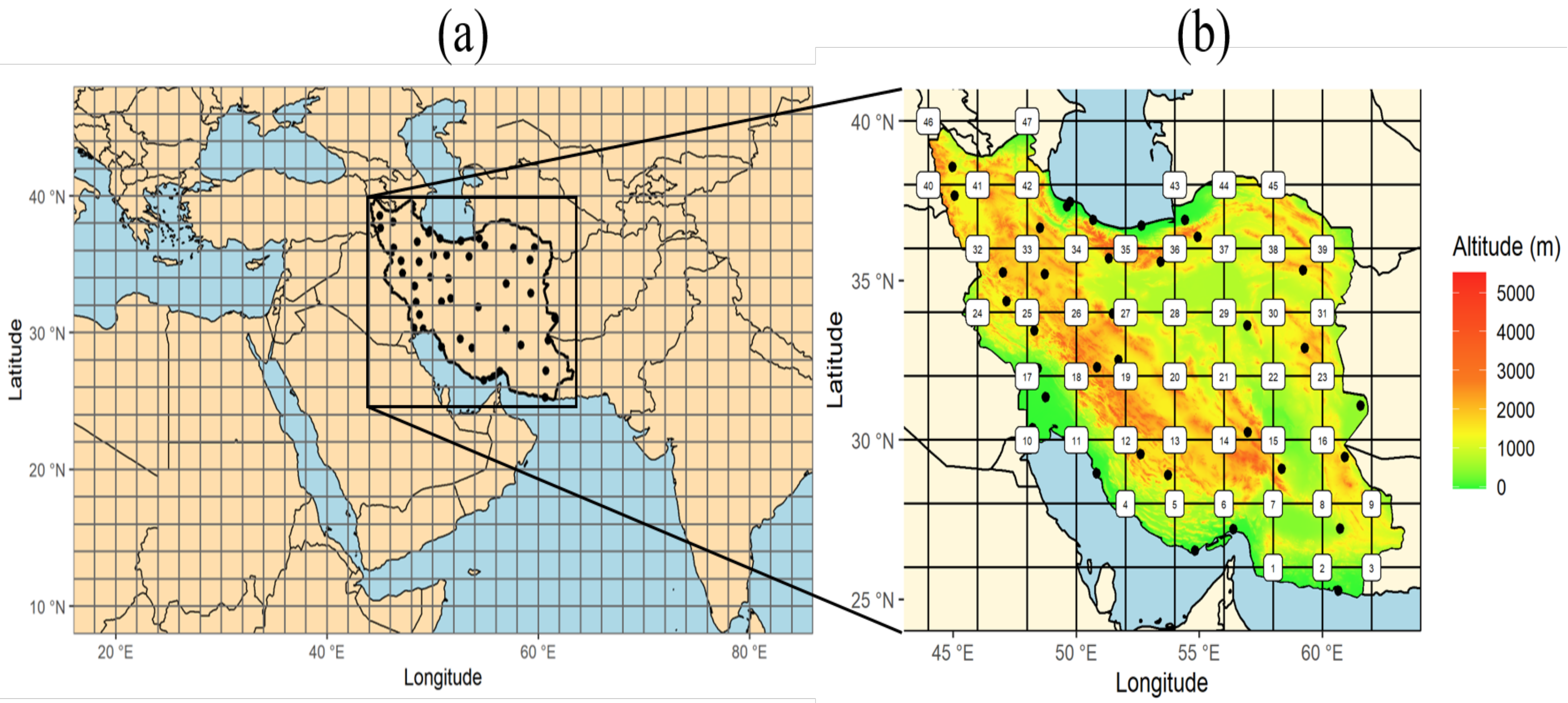
Data and Climatology

Much of Iran is affected by subtropical high pressure (STHP) and is therefore located in the desert belt of the Northern Hemisphere; however, climatic diversity in Iran is very high [45]. In the north and on the southern shores of the Caspian Sea, the climate is temperate and humid. In the western part of the country it is Mediterranean climate and in the southern regions, the hot semi-arid climate prevails. Due to the existence of Alborz mountains in the north and Zagros mountain ranges in the west of Iran, the interior of the Iranian plateau also has an arid and desert climate. The mean annual temperature increases from northwest to southeast, from about 10 °C in Azerbaijan region to 25–30 °C in the south and southeast [46]. Due to its geographical location, Iran’s average precipitation is much lower than the global average. More than two-thirds of Iran’s area has an average annual precipitation of less than 300 mm, but there are rainfall nuclei above 1000 mm in the Zagros region and the northern slopes of Alborz [47]. Results by Darand and Sohrabi [26] indicated significant changes in daily precipitation over more than 50% of Iran during the last two decades. This increasing trend is observed in the western and southwestern Iran.
We consider five climate variables over Middle East to avoid overfitting in calculating the PI-weights, while our focus is the annual maximum daily rainfall (AMP1) over Iran in this study. Table 1 lists five climate variables. Consecutive wet days and dry days are defined as consecutive days with daily precipitation of ≥1 and <1 mm, respectively [48,49]. These are recommended by the Expert Team on Climate Change Detection and Indices [44,50]. These five variables including four auxiliary variables are used to compute robustly the weights of independence of the CMIP6 models [40,42].
Table S1 in the accompanying Supplementary Materials lists the 24 CMIP6 climate models used in this study. The considered scenarios are shared socioeconomic pathways SSP2-4.5, SSP3-7.0, and SSP5-8.5 [30]. Three overlapping periods are considered for future data, namely, period 1 (2021–2050), period 2 (2046–2075), and period 3 (2071–2100), abbreviated by P1, P2, and P3 in this study. The reason why the periods overlap is to make each period at least 30 years long by the end of this century.
Figure 1 depicts maps of Middle East and Iran showing 42 observations sites and 47 points over 2 × 2 grids inside Iran. The observations for 44-year (1971–2014) reference period were obtained from the Iran Meteorological Organization. The reason why we choose 44-year reference period instead of 30-year is because there are the observations of 44 years over 42 stations in Iran. A sample size 44 is better than 30, both in estimating stably the parameters of GEV distribution and in applying the bias correction method. To re-grid and to construct a rain field on grid points of 2 × 2 , the Barnes scheme [51] was used for the observed time series and simulation data from the 24 CMIP6 models for each of five climate variables. In total, 598 grid points were used to cover Iran and its surrounding areas.
The remainder of this paper is structured as follows. The statistical methods are described in Section 2. The results of model weights and projected future changes in Iran are presented in Section 3. Discussions are then given in Section 4, followed by a conclusion in Section 5. Details including technical specifics, tables, and figures are provided in the accompanying Supplementary Materials.

2. Methods

2.1. Generalized Extreme Value Distribution

The generalized extreme value (GEV) distribution has been widely used to analyze extreme univariate values. The cumulative distribution function of the GEV distribution is as follows:
G ( x ) = e x p 1 + ξ x μ σ 1 / ξ ,
when 1 + ξ ( x μ ) / σ > 0 , where μ , σ , and ξ are the location, scale, and shape parameters, respectively, [20].
The changes in extremes is usually described in terms of the changes in extreme quantiles. These are computed by inverting the following (1): z p = μ σ ξ [ 1 { l o g ( 1 p ) } ξ ] , where G ( z p ) = 1 p . Here, z p is called as the return level associated with the return period 1 / p . The value z p is expected to be exceeded once every 1 / p years on average [20]. These quantities are defined for all values, but applied to extreme precipitation in this study. Conversely to the above, the return period T ( z ) = 1 / p for the given value z is obtained by calculating p ( z ) = 1 G ( z ) . For the given value z, T ( z ) is sometimes called the expected waiting time, and the value p ( z ) = 1 G ( z ) is referred to as the exceedance probability of z. The exceedance probability is often used as an alternative to the return period [53,54]. Another quantity that we can obtain is the expected number of reoccurrences during a certain period. By multiplying 30 years (for example) by the exceedance probability p ( z ) , we can estimate the expected frequency of such years over a period of 30 years in which we have more than z amount of AMP1 for a year.
The relative change of 20-year return level in the period P i for i = 1 , 2 , 3 relative to the reference period P 0 is defined as:
δ R 20 ( P i ) = R 20 ( P i ) R 20 ( P 0 ) R 20 ( P 0 ) × 100 ,
where R 20 ( P ) is the 20-year return level in the period P.
The parameters in GEV distribution are estimated by the maximum likelihood method [20,55] or the L-moment method [13]. In this study, we employ the latter, which is more efficient in small samples than the maximum likelihood estimator [13]. We used the “lmom” package in R [56].

2.2. Bias Correction

The simulated data are often associated with systematic biases of the simulation model. Such biases sometimes produce the historical data which are considerably different from the distribution of the observations. Bias-correction (BC) methods are sometimes employed to address this problem. A BC method transforms the simulated data into new data which have fewer biases with respect to an observed time series. To correct the model outputs more efficiently by taking account of the dependency among variables or nearby grids, several multivariate BC methods have been proposed. In this study, we chose the multivariate bias correction (MBC) method by Cannon [57] among the many available BC techniques [24,58]; it is a multivariate extension of quantile delta mapping (QDM). QDM has an advantage of preserving the approximate trends of the model data. The MBC is applied to the five climate variables provided in Table 1 to take into account the dependency among these variables. The method is not applied to the data of each period separately but to the whole data of all periods (2021–2100) at once. More details are provided in the Supplementary Materials.

2.3. Performance and Independence Weighting for Ensembles

Model averaging is a statistical method in which unequal or equal weights are assigned to those models. Despite some arguments, the equal weighting or “model democracy” [32] has been criticized because it does not consider the performance, uncertainty, and independency of each model in building an multi-model ensemble (MME) ([37,59,60], for example).
As the basic idea of PI-weighting, models that agree poorly with observations for a selected set of diagnostics receive less weight, as do models that largely duplicate existing models [39]. Weights are computed for each model based on a combination of the distance D i (apprising the performance) and the model similarity S i j (apprising the dependence):
w i = e x p ( D i σ D ) 1 + j i M e x p ( S i j σ S ) ,
with the total number of models M and the shape parameters σ D and σ S . The weights are normalized so that their sum equals 1.
The numerator represents the modeling skill when using a Gaussian weighting, where the weight decreases exponentially the farther away a model is from the observed data. The denominator is the “effective repetition of a model” [37] and is intended to account for the model interdependency [39].
To compute the performance of each model, T-year return levels are compared based on the GEV fitting on the historical data and the observations. To calculate the model similarity S i j , we follow a technique proposed by Sanderson et al. [61] that is based on the principle component analysis (PCA) applied to the simulation data only. This PCA is executed separately for each of five climate variables. Thus, we have five distances between models i and j. Then, the final distance are computed by averaging those five distances for models i and j.
The parameters σ D and σ S tune the strength of weighting and the relative significance of the performance and independence [42]. Large values will result in to an almost equal weights, whereas small values will cause aggressive (or one-sided) weights, providing most of the weight to a few models. The shape parameters are often determined through a perfect model test (or a model-as-truth experiment) using the continuous rank probability score [40,42]. This leave-one-out procedure needs a huge computing time. To overcome this computational burden, we follow a relatively simple method proposed by [43] to determine the shape parameters. More details in computing the distance S i j and in selecting the shape parameters are given in the Supplementary Materials.

3. Results

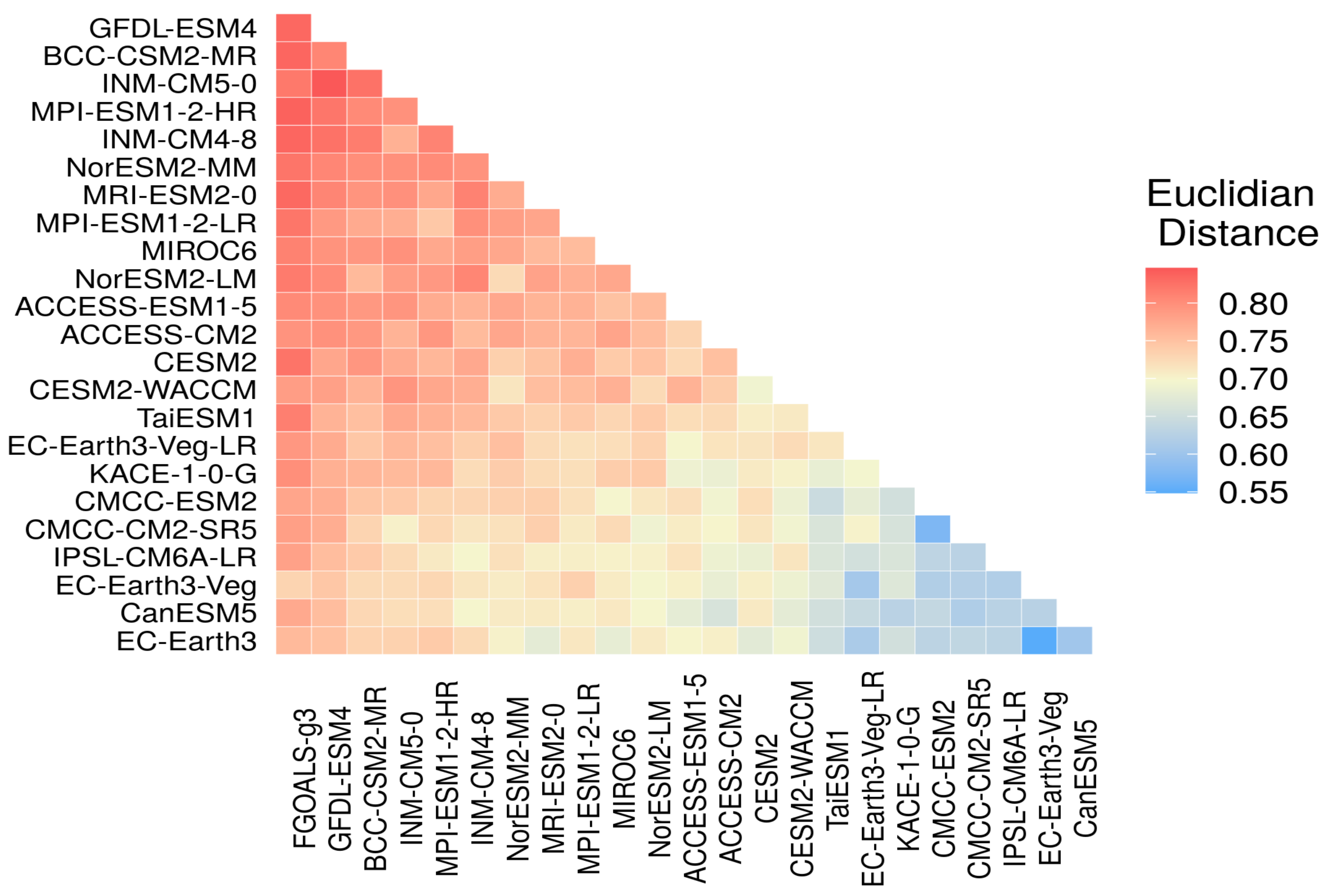
3.1. Model Similarity
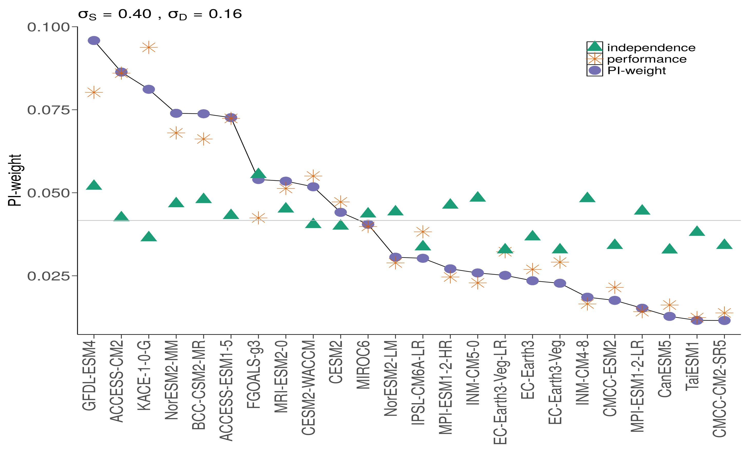
Table S2 provides the similarity values S i j for certain models. Figure 2 shows the intermodel distance matrix for the 24 CMIP6 models considered in this study. The distances are obtained from the five climate variables listed in Table 1 for the Middle East, using the historical data and the future simulation data. Each box shows a pairwise combination, where red color indicates a greater distance. According to Figure 2, models FGOALS-g3, GFDL-ESM4, BCC-CSM2-MR, INM-CM5-0, MPI-ESM1-2-HR, and NorESM2-MM were found to be the most independent, whereas models CanESM5, EC-Earth3-Veg, IPSL-CM6A-LR, and CMCC-CM2-SR5 were found to be the most dependent. The details on these models are available in Table S1 in the Supplementary Materials.

3.2. PI-Weights

The normalized PI-weights are obtained using Equation (3) with σ S = 0.4 and σ D = 0.16 . Figure 3 demonstrates the distributions of P-, I-, and PI-weights. The variability of I-weights is smaller than that of P-weights.
The high P-weight of the KACE-1-0-G decrease in the PI-weight owing to the low I-weight. The PI-weights of the GFDL-ESM4, NorESM2-MM, andBCC-CSM2-MR models increase owing to a relatively high independency. The PI-weight is not located in the middle of the P- and I-weights, but is close to the P-weight, except in a few cases. When the P-weight (I-weight) is almost the same as the equal weight, as in the FGOALS-g3 (ACCESS-CM2 and ACESS-ESM1-5) model, the PI-weight is wholly influenced by the I-weight (P-weight). The performances for some of the models, such as INM-CM4-8, CMCC-ESM2, MPI-ESM1-2-LR, CanESM5, TaiESM1, and CMCC-CM2-SR5 are so low that their (even relatively high) I-weights do not affect the final weights. Based on this view, the performance is more influential to the PI-weights than the independency. Some of these observations may be changed if different σ S and σ D are used.

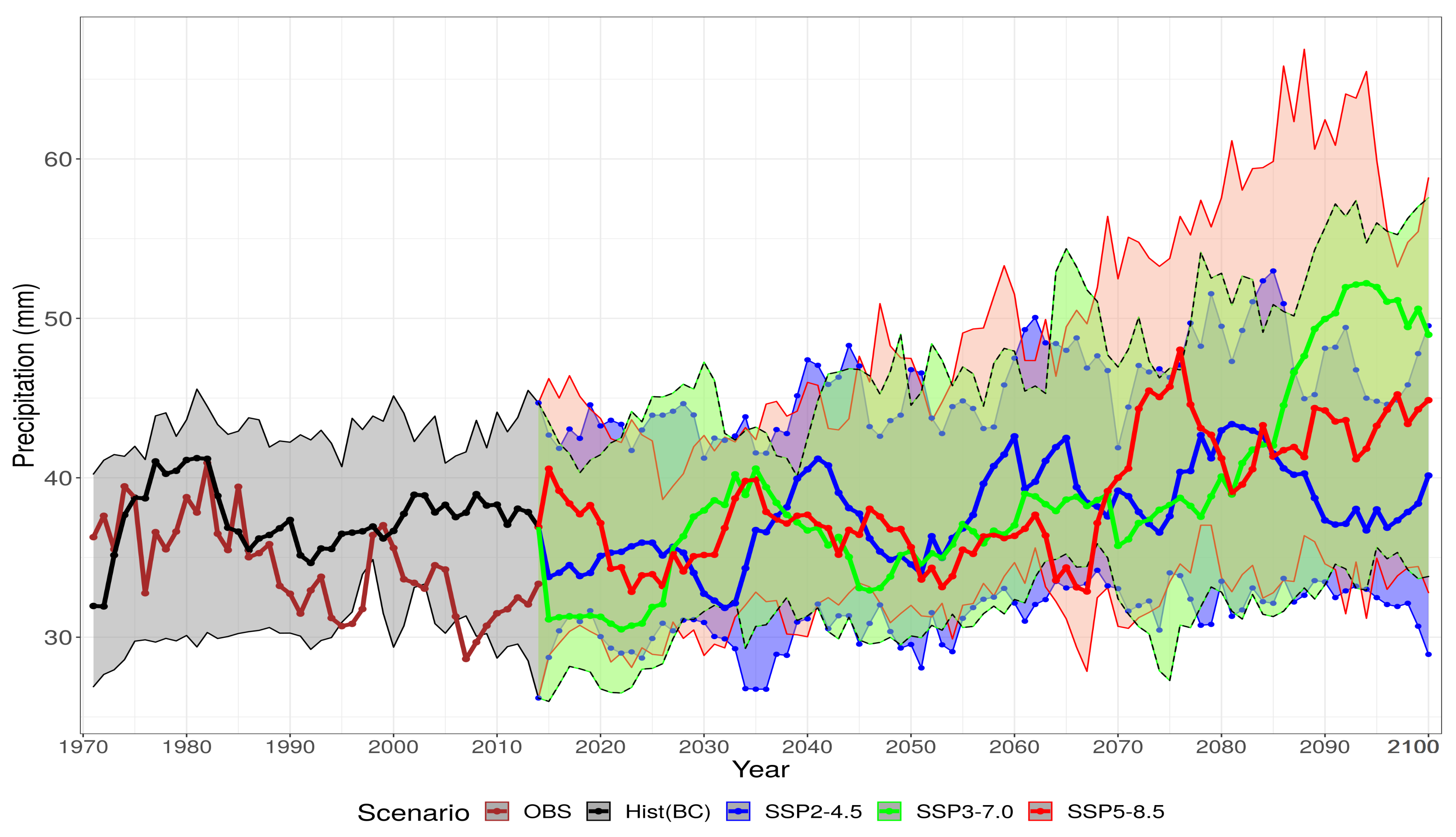
3.3. Future Projection of Extreme Precipitation
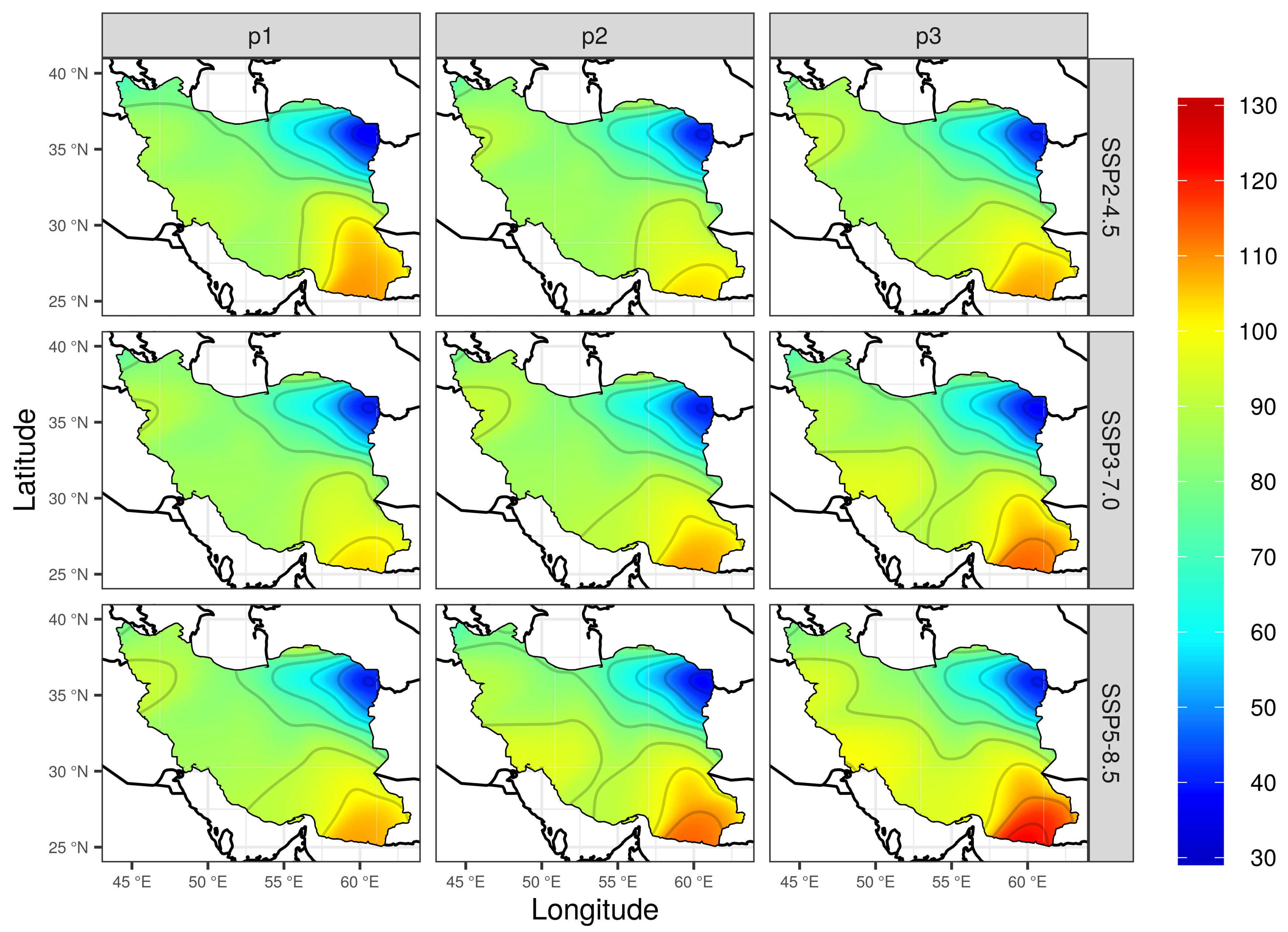
Using the PI-weights obtained in the above section, the future extreme precipitations are projected by the MME. Note that the future climate data are used after the bias correction with the MBC method [57]. Figure 4 illustrates the time series plots of the 9-year moving averages of AMP1 in Tehran with a 90% confidence band, from the observations, from the PI-weighted MME of the historical data, and from the PI-weighted averages for the future simulation data under the three SSP scenarios. Lower 5% and upper 5% prediction values among 24 models are lined to construct 90% confidence band. In Figure 4, the line for the observations shows more variation than the lines of bias-corrected historical data by the PI-weighted MME. The variance of 9-year moving averages of observed AMP1 is 4.98, whereas that value for the PI-weighted ensemble of bias-corrected historical data is 1.93.

3.4. Return Levels

Figure 5 (S3) displays boxplots of the 20-year (50-year) return levels of the AMP1 in Iran. The boxplot of the historical data after BC is similar to that from the observations, whereas the boxplot before BC is much smaller than that from the observations. The increasing trends from P1 to P3 are evident in every scenario. This result is consistent with that by Darand [24]. Summary statistics of the corresponding values of these boxplots are provided in Table S3.
Figure 6 shows isopluvial maps of the 50-year return levels of the AMP1 for three future periods under the three scenarios. Increasing trends from P1 to P3 in SSP3-7.0 and SSP5-8.5 scenarios are predicted in the western and southwestern parts of Iran, which is consistent with the result by Darand and Sohrabi [26].

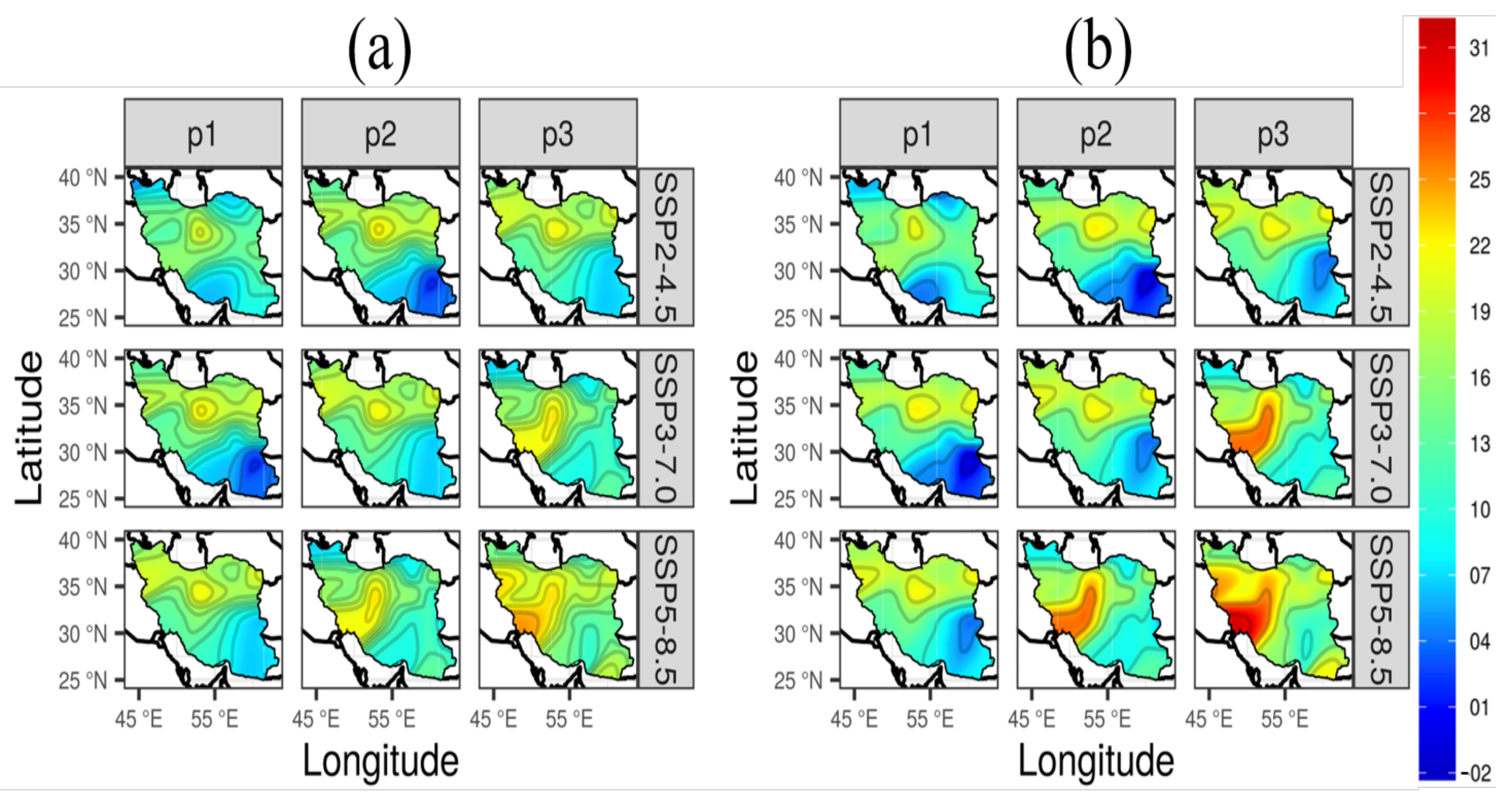
3.5. Changes in Return Levels

Figure 7 exhibits relative changes (unit: %) of the 20- and 50-year return levels of extreme precipitation over Iran relative to the years 1971–2014. The increasing changes are more evident in the northern part than in the southern area. Summary statistics of relative changes are presented in Table S4 in the Suplementary Materials. Relative increases in the observations for spatially averaged 20-year (50-year) return level are approximately 15.6% (17.5%) in the SSP2-4.5, 23.2% (25.2%) in the SSP3-7.0, and 28.7% (30.0%) in the SSP5-8.5 scenario by the year 2100.

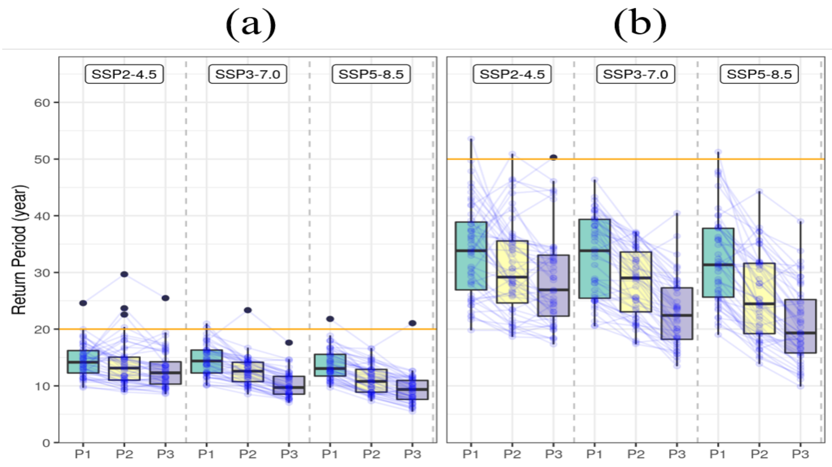
3.6. Change in Return Periods

Figure 8 displays boxplots for the 20-year and 50-year return periods, as compared to the reference years (1971–2014) for the three future periods under the three scenarios. The corresponding statistics are presented in Table 2. We realize that a 1-in-20 year (1-in-50 year) AMP1 in Iran will likely become 1-in-12 (1-in-26) year, 1-in-10 (1-in-22) year, and 1-in-9 (1-in-20) year events in the median by 2100 based on the SSP2-4.5, SSP3-7.0, and SSP5-8.5 scenarios, respectively, as compared to the observations from 1971 to 2014. These findings indicate that both return periods are likely to decrease on average by approximately 54% under the SSP2-4.5 and 57% under the SSP5-8.5 by the year 2100.

3.7. Exceedance Probability and Waiting Time

The spatially averaged estimates of the exceedance probability are presented in Figure S5 and Table S5. There are relatively large differences in the exceedance probability of a rainfall of 50 to 80 mm compared with that for over 80 mm, as shown in Figure S6. The differences between the past and future scenarios are distinct during the period P3.
The expected waiting time ( T ( z ) ) until the reoccurrence of a specific AMP1 value (z) are listed in Table 3. For z = 50 mm of rainfall, for example, the expected waiting times until a reoccurrence are 28 years in the past, 13.0 years in the future period P1, 10.8 years in P2, and 7.9 years in P3 based on the SSP5-8.5 scenario.

3.8. Expected Number of Reoccurring Years

The expected number of years of occurrence are given in Table S6. For z = 50 mm, as a specific example, during the last 30 years, we have experienced 0.9 year in which AMP1 was greater than 50 mm. In addition, we are likely to have an expected number of years of 2.3 for the future period P1, 2.8 for P2, and 3.8 for P3 under the SSP5-8.5 scenario.
From this comparison, particularly for AMP1 of 50mm, the expected number of years of occurrence for the future periods under the SSP5-8.5 scenario increases by approximately 2.5 (3.1) times that over the last 30 years for P1 (P2), and 4.2 times that for P3 by the end of 21st century. These results are based on the spatially averaged values. When the exceedance probability is considered for each grid, different local results will be obtained.

4. Discussion

It is accepted in general that increasing greenhouse gases induce atmospheric temperature warming, which leads to increasing equivalent humidity, according to the Clausius–Clapeyron relationship [8]. The increase in atmospheric water vapor is the main factor in generating convective instability.
Zarrin and Dadashi-Roudbari [29] concluded that the trend and slope of the intensity of extreme precipitation are increasing by the year 2100 in all zones in Iran except for some areas (BWh, BWk, and Cfa zones) for SSP1-2.6 and SSP3-7.0 scenarios. Our result shows that the increasing trend of the AMP1 is projected in the western and southwestern parts of Iran. Based on Figure 6 of this study, there seems no change from P1 to P3 in Cfa zone, which leads to the same result by two studies. In Bwh and BWk zones, our result shows that there are no changes for SSP2-4.5 scenario, but increasing trends for SSP3-7.0 and SSP5-8.5 scenarios. Thus, it seems hard to compare two results directly. However, an agreement in general between two studies is that the increasing trend of extreme precipitation is projected over Iran except for some area.
The daily precipitation data consist of measurements from 00:00 to 24:00 throughout the day. In daily observations, the rainfall does not accumulate between 22:00 and 02:00, for example. In the data used in this study, such precipitation is divided and recorded in two separate days. The actual serious daily risk due to heavy rainfall does not exactly depend on the precipitation over a time duration from 00:00 to 24:00 exclusively. It is therefore recommended to consider the AMP1 data based on the maximum precipitation during the 24 h movement. In this sense, the results presented in this study underestimate the actual intensity and frequency of AMP1. More realistic daily data, such those as obtained after moving for 24 h and the annual maximum of two (and several) days of precipitation, should be used in a future study for assessment of risk owing to extreme rainfall.
Brunner et al. [42,62] considered multiple observational (or reanalysis) datasets to include an estimate of the observational uncertainty. They proposed a novel approach to account for the observational spread and uncertainty in a multi-model weighting study, which can lead to robust result and a more precise uncertainty quantification. In addition, considering multiple observational datasets may address the problem in which the BC and performance-based weighting scheme utilize an excessive number of observations. We believe that using the observations twice in the BC and weight calculation is unadvisable. Xu et al. [34] considered a Bayesian weighting method that removes observations during the initial phase of the downscaling and adds them in the estimation of posterior distribution. However, if the series of observations is sufficiently long to divide into two parts, we may use one part for the BC and the other part for weights calculation. Although we did not apply these methods, this would be a good approach in a future study.

5. Conclusions

We estimated the future changes in precipitation extremes within Iran using observations, 24 multiple CMIP6 models, generalized extreme value distribution, the multivariate bias correction technique, and the model weighting method (PI-weighting), which account for both the performance and independence of the models. To avoid overfitting in the PI-weighting, we considered five climate variables over Middle East.
In applying the PI-weighting method, we follow ways of selecting two shape parameters [43], based on the p-value of the chi-square statistic and entropy. The methods are simple and intuitively appealing, although they may need more justification to use.
From 20-year and 50-year return levels of the annual maximum daily precipitation (AMP1) averaged over 47 grids in Iran for three future periods under three SSP scenarios, the increasing trends from P1 (2021–2050) to P3 (2071–2100) are evident in SSP3-7.0 and SSP5-8.5 scenario. This result is somehow consistent with that of Darand [24]. We predict that the relative increases of 20-year return level of the AMP1 in the spatial median from the past observations to the year 2100 will be approximately 15.6% in the SSP2-4.5, 23.2% in the SSP3-7.0, and 28.7% in the SSP5-8.5 scenarios, respectively.
From the analysis described in this study, we realized that a 1-in-20 year (1-in-50 year) AMP1 within Iran will likely become a 1-in-12 (1-in-26) year, a 1-in-10 (1-in-22) year, and a 1-in-9 (1-in-20) year event in terms of the median by the year 2100 under the SSP2-4.5, SSP3-7.0, and SSP5-8.5 scenarios, respectively, as compared to the observed data from 1971 through 2014. The increasing trend is projected in the western and southwestern parts of Iran.
The expected frequency of the reoccurring years, particularly for AMP1 about 50 mm under the SSP5-8.5 scenario, is predicted to increase by approximately 2.5 times that of the past 30 years for period 1 (2021–2050), about 3.1 times that for period 2 (2046–2075), and approximately 4.2 times that for period 3 (2071–2100).
Heavy rainfall can have a significant effect on human life, communities, infrastructure, agriculture, and natural ecosystems. Thus, in addressing the impact of climate change due to more frequent extreme precipitation events, governments and communities should prepare the proper infrastructure and systems more carefully and securely to prevent critical damage, such as loss of life from landslides and flooding.

Supplementary Materials

The following are available at https://www.mdpi.com/article/10.3390/atmos12081052/s1. Table S1: The list of 24 CMIP6 (Coupled Model Intercomparison Project Phase 6) models analyzed in this study. Table S2: The similarity distance metric S i j between model i and model j. Table S3: Statistics of 20-year and 50-year return levels of the annual largest daily rainfall (unit: mm) averaged over 47 grids in Iran for the observations (OBS) and the future periods under the three SSP scenarios. Table S4: Relative change (unit: %) in 20-year and 50-year return levels of the annual largest daily rainfall averaged over Iran relative to 1971–2014. Table S5: Spatially averaged the exceedance probability over Iran for the annual maximum daily precipitation (AMP1) from 20 m m to 100 m m , obtained from the observations (OBS) and the CMIP6 models. Table S6: The expected frequency of reoccurring years during 30 years for specific the annual maximum daily precipitation (AMP1) values from 20 m m to 100 m m in Iran, obtained from the observations (OBS) and the CMIP6 models. Figure S1: Plot of the entropy as σ S changes from 0.1 to 1.0. Figure S2: Examples of time series plots of the observations (blue line), CMIP6 data (green line), and the bias-corrected data (red line) in Iran. Figure S3: Arrangement of data and 7-year moving averages composed of the historical data from 1850 to 2014 and the future data for computing the Spearman correlation coefficient between models. Figure S4: Box-plots of 50-year return levels of the annual largest daily rainfall (unit: mm) averaged over 47 grids in Iran for the future periods under the three SSP scenarios. Figure S5: The exceedance probability plots for the annual maximum daily precipitation (AMP1) from 20 mm to 100 mm in Iran, obtained from the observations (OBS) and the CMIP6 models.

Author Contributions

Conceptualization, K.J. and J.-S.P.; methodology, Y.S. and J.-S.P.; software, J.H. and Y.S.; validation, K.J.; investigation, J.H. and J.-S.P.; data curation, K.J. and J.H.; writing—original draft preparation, Y.S. and J.-S.P.; writing—review and editing, J.-S.P.; visualization, Y.S. and J.H.; supervision, J.-S.P.; project administration, K.J. and J.-S.P.; funding acquisition, K.J. and J.-S.P. All authors have read and agreed to the published version of the manuscript.

Funding

This study was supported by a National Research Foundation of Korea (NRF) grant funded by the Korean government (MSIT) (No.2020R1I1A3069260) and the BK21 FOUR (Fostering Outstanding Universities for Research, NO.5120200913674) funded by the Ministry of Education (MOE, Korea) and National Research Foundation of Korea (NRF).

Institutional Review Board Statement

Not applicable.

Informed Consent Statement

Not applicable.

Data Availability Statement

The CMIP data are available through ESGF’s website at https://esgf-node.llnl.gov/projects/ (accessed on 29 March 2021) and DKRZ’s website at https://cera-www.dkrz.de/WDCC/ui/cerasearch/ (accessed on 29 March 2021). Observational station data in Iran are provided by Iran Meteorological Organization at https://irandataportal.syr.edu/iran-meteorological-organization/ (accessed on 11 January 2021).

Acknowledgments

The authors would like to thank the reviewers and the editors of the special issue for their comments and suggestions, which have importantly improved this paper. We acknowledge the World Climate Research Program Working Group on Coupled Modeling, which is responsible for CMIP, and we thank the climate modeling groups for producing and making available their model outputs. For CMIP, the U.S. DoE Program for Climate Model Diagnosis and Intercomparison provided coordinating support and led the development of the software infrastructure in partnership with the Global Organization for Earth System Science Portals. We are grateful to all contributors to the R packages, which were important for this work. The authors thank Yire Shin who provided valuable help for this paper.

Conflicts of Interest

The authors declare that they have no conflict of interest.

References

  1. IPCC. Managing the Risks of Extreme Events and Disasters to Advance Climate Change Adaptation. Special Report of the Intergovernmental Panel on Climate Change; Cambridge University Press: Cambridge, UK, 2012; Available online: http://ipcc-wg2.gov/SREX/report/ (accessed on 15 July 2020).
  2. Easterling, D.R.; Kunkel, K.E.; Arnold, J.R.; Knutson, T.; LeGrande, A.N.; Leung, L.R.; Vose, R.S.; Waliser, D.E.; Wehner, M.F. Precipitation Change in the United States. In Climate Science Special Report: Fourth National Climate Assessment; Wuebbles, D.J., Fahey, D.W., Hibbard, K.A., Dokken, D.J., Stewart, B.C., Maycock, T.K., Eds.; U.S. Global Change Research Program: Washington, DC, USA, 2017; Volume I, pp. 207–230. [Google Scholar] [CrossRef]
  3. Westra, S.; Alexander, L.V.; Zwiers, F.W. Global increasing trends in annual maximum daily precipitation. J. Clim. 2013, 26, 3904–3918. [Google Scholar] [CrossRef] [Green Version]
  4. Freychet, N.; Hsu, H.; Chou, C.; Wu, C. Asian summer monsoon in CMIP5 projections: A link between the change in extreme precipitation and monsoon dynamics. J. Clim. 2015. [Google Scholar] [CrossRef]
  5. Alexander, L.V. Global observed long-term changes in temperature and precipitation extremes: A review of progress and limitations in IPCC assessments and beyond. Weather. Clim. Extrem. 2016, 11, 4–16. [Google Scholar] [CrossRef] [Green Version]
  6. Park, C.; Min, S.K.; Lee, D.; Cha, D.H.; Suh, M.S.; Kang, H.K.; Hong, S.Y.; Lee, D.K.; Baek, H.J.; Boo, K.O.; et al. Evaluation of multiple regional climate models for summer climate extremes over East Asia. Clim. Dynam. 2016, 46, 2469–2486. [Google Scholar] [CrossRef]
  7. Dike, V.N.; Lin, Z.-H.; Ibe, C.C. Intensification of Summer Rainfall Extremes over Nigeria during Recent Decades. Atmosphere 2020, 11, 1084. [Google Scholar] [CrossRef]
  8. Ruckstuhl, C.; Philipona, R.; Morl, J.; Ohmura, A. Observed relationship between surface specific humidity, integrated water vapor, and longwave downward radiation at different altitudes. J. Geophys. Res. Atmos. 2007, 112, 1–7. [Google Scholar] [CrossRef]
  9. Lenderink, G.; van Meijgaard, E. Increase in hourly precipitation extremes beyond expectations from temperature changes. Nat. Geosci. 2008, 1, 511–514. [Google Scholar] [CrossRef]
  10. Berg, P.; Moseley, C.; Haerter, J.O. Strong increase in convective precipitation in response to higher temperatures. Nat. Geosci. 2013, 6, 181–185. [Google Scholar] [CrossRef]
  11. Scott, M.; Prepare for More Downpours: Heavy Rain Has Increased across Most of the United States, and Is Likely to Increase Further. ClimateWatch Magazine. 2019. Available online: https://www.climate.gov/news-features/featured-images/prepare-more-downpours-heavy-rain-has-increased-across-most-united-0 (accessed on 25 July 2020).
  12. Mann, M.E.; Kump, L.R. Dire Predictions: Understanding Climate Change, 2nd ed.; DK Publishing: New York, NY, USA, 2015. [Google Scholar]
  13. Hosking, J.R.M.; Wallis, J.R. Regional Frequency Analysis: An Approach Based on L-Moments; Cambridge University Press: Cambridge, UK, 1997; 244p. [Google Scholar]
  14. El Adlouni, S.; Ouarda, T.B.; Zhang, X.; Roy, R.; Bobée, B. Generalized maximum likelihood estimators for the nonstationary generalized extreme value model. Water Resour. Res. 2007, 43, W03410. [Google Scholar] [CrossRef]
  15. Park, J.-S.; Kang, H.-S.; Lee, Y.; Kim, M.-K. Changes in the extreme daily rainfall in South Korea. Intern. J. Climatol. 2011, 31, 2290–2299. [Google Scholar] [CrossRef]
  16. Kharin, V.V.; Zwiers, F.W.; Zhang, X.; Wehner, M. Changes in temperature and precipitation extremes in the CMIP5 ensemble. Clim. Chang. 2013, 119, 345–357. [Google Scholar] [CrossRef]
  17. Zhu, J.; Forsee, W.; Schumer, R.; Gautam, M. Future projections and uncertainty assessment of extreme rainfall intensity in the United States from an ensemble of climate models. Clim. Chang. 2013, 118, 469–485. [Google Scholar] [CrossRef]
  18. Gentilucci, M.; Barbieri, M.; Lee, H.S.; Zardi, D. Analysis of rainfall trends and extreme precipitation in the Middle Adriatic Side, Marche Region (Central Italy). Water 2019, 11, 1948. [Google Scholar] [CrossRef] [Green Version]
  19. Lee, Y.; Shin, Y.G.; Park, J.S.; Boo, K.O. Future projections and uncertainty assessment of precipitation extremes in the Korean peninsula from the CMIP5 ensemble. Atmos. Sci. Lett. 2020, e954. [Google Scholar] [CrossRef] [Green Version]
  20. Coles, S. An Introduction to Statistical Modelling of Extreme Values; Springer: New York, NY, USA, 2001; p. 224. [Google Scholar]
  21. Modarres, R.; Sarhadi, A. Rainfall trends analysis of Iran in the last half of the twentieth century. J. Geophys. Res. Atmos. 2009, 114, D3. [Google Scholar] [CrossRef]
  22. Rahimi, M.; Fatemi, S.S. Mean versus Extreme Precipitation Trends in Iran over the Period 1960–2017. Pure Appl. Geophys. 2019, 176, 3717–3735. [Google Scholar] [CrossRef]
  23. Shokouhi, M.; Nejad, S.H.S.; Aval, M.B. Evaluation of simulated precipitation and temperature from CMIP5 climate models in regional climate change studies (case study: Major rainfed wheat–production areas in Iran). J. Water Soil 2018, 32, Pe1013–Pe1027. [Google Scholar]
  24. Darand, M. Projected changes in extreme precipitation events over Iran in the 21st century based on CMIP5 models. Clim. Res. 2020, 82, 75–95. [Google Scholar] [CrossRef]
  25. Abbaspour, K.C.; Faramarzi, M.; Ghasemi, S.S.; Yang, H. Assessing the impact of climate change on water resources in Iran. Water Resour. Res. 2009, 45, W10434. [Google Scholar] [CrossRef] [Green Version]
  26. Darand, M.; Sohrabi, M.M. Identifying drought and flood–prone areas based on significant changes in daily precipitation over Iran. Nat. Hazards 2018, 90, 1427–1446. [Google Scholar] [CrossRef]
  27. Maghsood, F.F.; Moradi, H.; Bavani, M.; Reza, A.; Panahi, M.; Berndtsson, R.; Hashemi, H. Climate Change Impact on Flood Frequency and Source Area in Northern Iran under CMIP5 Scenarios. Water 2019, 11, 273. [Google Scholar] [CrossRef] [Green Version]
  28. Rahimi, J.; Laux, P.; Khalili, A. Assessment of climate change over Iran: CMIP5 results and their presentation in terms of Koppen–Geiger climate zones. Theor. Appl. Climatol. 2020, 141, 1–17. [Google Scholar] [CrossRef]
  29. Zarrin, A.; Dadashi-Roudbari, A. Projection of future extreme precipitation in Iran based on CMIP6 multi-model ensemble. Theor. Appl. Climatol. 2021, 144, 643–660. [Google Scholar] [CrossRef]
  30. O’Neill, B.C.; Kriegler, E.; Riahi, K.; Ebi, K.L.; Hallegatte, S.; Carter, T.R.; Mathur, R.; van Vuuren, D.P. A new scenario framework for climate change research: The concept of Shared Socioeconomic Pathways. Clim. Chang. 2014, 122, 387–400. [Google Scholar] [CrossRef] [Green Version]
  31. Tebaldi, C.; Hayhoe, K.; Arblaster, J.M.; Meehl, G.A. Going to the extremes: An intercomparison of model-simulated historical and future changes in extreme events. Clim. Chang. 2006, 79, 185–211. [Google Scholar] [CrossRef]
  32. Knutti, R. The end of model democracy? Clim. Chang. 2010, 102, 394–404. [Google Scholar] [CrossRef]
  33. Suh, M.S.; Oh, S.G.; Lee, D.K.; Cha, D.H.; Choi, S.-J.; Jin, C.-S.; Hong, S.-Y. Development of new ensemble methods based on the performance skills of regional climate models over South Korea. J. Clim. 2012, 25, 7067–7082. [Google Scholar] [CrossRef] [Green Version]
  34. Xu, D.; Ivanov, V.; Kim, J.; Fatichi, S. On the use of observations in assessment of multi-model climate ensemble. Stoch. Environ. Res. Risk Assess. 2019, 33, 1923–1937. [Google Scholar] [CrossRef]
  35. Baker, N.C.; Taylor, P.C. A framework for evaluating climate model performance metrics. J. Clim. 2016, 29, 1773–1782. [Google Scholar] [CrossRef]
  36. Georgi, F.; Mearns, L.O. Calculation of average, uncertainty range and reliability of regional climate changes from AOGCM simulations via the ’Reliability Ensemble Averaging (REA)’ method. J. Clim. 2002, 15, 1141–1158. [Google Scholar] [CrossRef]
  37. Sanderson, B.M.; Knutti, R.; Caldwell, P. A representative democracy to reduce interderpendency in a multimodel ensemble. J. Clim. 2015, 28, 5171–5194. [Google Scholar] [CrossRef] [Green Version]
  38. Abramowitz, G.; Gupta, H. Toward a model space and model independence metric. Geophys. Res. Lett. 2008, 35, L05705. [Google Scholar] [CrossRef] [Green Version]
  39. Knutti, R.; Sedlacek, J.; Sanderson, B.M.; Lorenz, R.; Fischer, E.M.; Eyring, V. A climate model projection weighting scheme accounting for performance and independence. Geophys. Res. Lett. 2017, 44, 1909–1918. [Google Scholar]
  40. Lorenz, R.; Herger, N.; Sedlacek, J.; Eyring, V.; Fischer, E.M.; Knutti, R. Prospects and caveats of weighting climate models for summer maximum temperature projections over North America. J. Geophys. Res. Atmos. 2018, 123, 4509–4526. [Google Scholar] [CrossRef]
  41. Shin, Y.; Lee, Y.; Park, J.S. A Weighting Scheme in A Multi-Model Ensemble for Bias-Corrected Climate Simulation. Atmosphere 2020, 11, 775. [Google Scholar] [CrossRef]
  42. Brunner, L.; Lorenz, R.; Zumwald, M.; Knutti, R. Quantifying uncertainty in European climate projections using combined performance-independence weighting. Environ. Res. Lett. 2019, 14, 124010. [Google Scholar] [CrossRef]
  43. Shin, Y.; Shin, Y.; Hong, J.; Kim, M.-K.; Byun, Y.-H.; Boo, K.-O.; Chung, I.-U.; Park, D.-S.R.; Park, J.-S. Future Projections and Uncertainty Assessment of Precipitation Extremes in the Korean Peninsula from the CMIP6 Ensemble with a Statistical Framework. Atmosphere 2021, 12, 97. [Google Scholar] [CrossRef]
  44. Zhang, X.; Alexander, L.; Hegerl, G.C.; Jones, P.; Tank, A.K.; Peterson, T.C.; Trewin, B.; Zwiers, F.W. Indices for monitoring changes in extremes based on daily temperature and precipitation data. Wiley Interdiscip. Rev. Clim. Chang. 2011, 2, 851–870. [Google Scholar] [CrossRef]
  45. Modarres, R.; Sarhadi, A.; Burn, D.H. Changes of extreme drought and flood events in Iran. Glob. Planet. Chang. 2016, 144, 67–81. [Google Scholar] [CrossRef]
  46. Rahimi, M.; Mohammadian, N.; Vanashi, A.R.; Whan, K. Trends in indices of extreme temperature and precipitation in Iran over the period 1960–2014. Open J. Ecol. 2018, 8, 396. [Google Scholar] [CrossRef] [Green Version]
  47. Alijani, B.; O’brien, J.; Yarnal, B. Spatial analysis of precipitation intensity and concentration in Iran. Theor. Appl. Climatol. 2008, 94, 107–124. [Google Scholar] [CrossRef]
  48. Karl, T.R.; Nicholls, N.; Ghazi, A. CLIVAR/GCOS/WMO workshop on indices and indicators for climate extremes: Workshop summary. Weather. Clim. Extrem. 1999, 42, 3–7. [Google Scholar]
  49. Peterson, T.C.; Foll, C.; Gruza, G.; Hogg, W.; Mokssit, A.; Plummer, N. Report on the Activities of the Working Group on Climate Change Detection and Related Rapporteurs 1998–2001; Rep. WCDMP-47, WMO-TD 1071; WMO: Geneve, Switzerland, 2001; 143p, Available online: https://www.clivar.org/sites/default/files/documents/048_wgccd.pdf (accessed on 15 November 2020).
  50. Ávila, Á.; Guerrero, F.C.; Escobar, Y.C.; Justino, F. Recent Precipitation Trends and Floods in the Colombian Andes. Water 2019, 11, 379. [Google Scholar] [CrossRef] [Green Version]
  51. Koch, S.E.; DesJardins, M.; Kocin, P.J. An interactive Barnes objective map analysis scheme for use with satellite and conventional data. J. Clim. Appl. Meteorol. 1983, 22, 1487–1503. [Google Scholar] [CrossRef]
  52. Hadley, W.; Winston, C.; Lionel, H.; Thomas, L.P.; Kohske, T.; Claus, W.; Kara, W.; Hiroaki, Y.; Dewey, D. ggplot2. R Package, Version 3.3.5. 2021. Available online: https://CRAN.R-project.org/package=ggplot2 (accessed on 3 July 2021).
  53. Serinaldi, F. Dismissing return periods! Stoch. Environ. Res. Risk Assess. 2015, 29, 1179–1189. [Google Scholar] [CrossRef] [Green Version]
  54. Paciorek, C.J.; Stone, D.A.; Wehner, M.F. Quantifying statistical uncertainty in the attribution of human influence on severe weather. Weather. Clim. Extrem. 2018, 20, 69–80. [Google Scholar] [CrossRef]
  55. Wilks, D. Statistical Methods in the Atmospheric Sciences, 3rd ed.; Academic Press: New York, NY, USA, 2011. [Google Scholar]
  56. Hosking, J.R.M. L-Moments. R Package, Version 2.8. 2019. Available online: https://CRAN.R-project.org/package=lmom (accessed on 5 March 2020).
  57. Cannon, A.J. Multivariate quantile mapping bias correction: An N-dimensional probability density function transform for climate model simulations of multiple variables. Clim. Dyn. 2018, 50, 31–49. [Google Scholar] [CrossRef] [Green Version]
  58. Maraun, D.; Widmann, M. Statistical Downscaling and Bias Correction for Climate Research; Cambridge University Press: Cambridge, UK, 2018. [Google Scholar]
  59. Massoud, E.C.; Espinoza, V.; Guan, B.; Waliser, D.E. Global Climate Model Ensemble Approaches for Future Projections of Atmospheric Rivers. Earth’s Future 2019, 7, 1136–1151. [Google Scholar] [CrossRef] [Green Version]
  60. Eyring, V.; Cox, P.M.; Flato, G.M.; Gleckler, P.J.; Abramowitz, G.; Caldwell, P.; William, D.C.; Bettina, K.G.; Alex, D.H.; Forrest, M.H.; et al. Taking climate model evaluation to the next level. Nat. Clim. Chang. 2019, 9, 102–110. [Google Scholar] [CrossRef] [Green Version]
  61. Sanderson, B.M.; Knutti, R.; Caldwell, P. Addressing interdependency in a multimodel ensemble by interpolation of model properties. J. Clim. 2015, 28, 5150–5170. [Google Scholar] [CrossRef]
  62. Brunner, L.; Pendergrass, A.G.; Lehner, F.; Merrifield, A.L.; Lorenz, R.; Knutti, R. Reduced global warming from CMIP6 projections when weighting models by performance and independence. Earth Syst. Dyn. Discuss. 2020, 11, 995–1012. [Google Scholar] [CrossRef]
Figure 1. (a) Map of the Middle East showing 42 observations sites inside Iran and 598 grid points over the whole area. The Barnes interpolation method was used to re-grid and to build a rainfall field over 2 × 2 grids in Middle East. (b) Map of the Iran from 44 to 62 longitude and 26 to 40 latitude, including the sea and land, with 47 grid points of 2 × 2 for this study. This map was drawn by using a R package ’ggplot2’ [52].
Atmosphere 12 01052 g001
Figure 2. A heatmap of the intermodel distance matrix, computed from the five climate variables for the Middle East, using the historical data and the future simulation data, for the 24 Coupled Model Inter-Comparison Project Phase (CMIP) 6 models. Each box shows a pairwise combination, where red color show a greater independence and blue color show a greater dependence.
Atmosphere 12 01052 g002
Figure 3. Distribution of the weights for the 24 CMIP6 models calculated based on the performance only (asterisk), the independence only (triangle), and both the performance and independence (circle). The weights are computed from the five climate variables for the Middle East.
Atmosphere 12 01052 g003
Figure 4. Time series plots of 9-year moving averages of the annual largest daily rainfall in Tehran from the observed data (dark brown line), from the PI-weighted ensemble of the bias-corrected historical data (black line) of the 24 CMIP6 models for the past years (1971–2014), and the PI-weighted averages for the bias-corrected future data under the three shared socioeconomic pathway (SSP) scenarios. Shaded bands show 90% confidence intervals. The blue, green, and red lines for the future are for SSP2-4.5, for SSP3-7.0, and for SSP5-8.5, respectively. The weights are computed from the five climate variables for Middle East.
Atmosphere 12 01052 g004
Figure 5. Boxplots of 20-year return levels (unit: mm) of the annual largest daily rainfall averaged over 47 grids in Iran for the future periods, namely P1 (2021–2050), P2 (2046–2075), and P3 (2071–2100), under the SSP2-4.5, SSP3-7.0, and SSP5-8.5 scenarios. OBS and HIST(NBC) stand for the observations and the historical data without a bias correction, respectively.
Atmosphere 12 01052 g005
Figure 6. Isopluvial maps of the 50-year return levels (unit: mm) of the annual largest daily rainfall for 47 grids over Iran for the future periods, namely, P1 (2021–2050), P2 (2046–2075), and P3 (2071–2100) under the SSP2-4.5, SSP3-7.0 and SSP5-8.5 scenarios.
Atmosphere 12 01052 g006
Figure 7. Isopluvial maps of for the relative changes (unit: %) of (a) 20-year and (b) 50-year return levels relative to 1971–2014 for the annual largest daily rainfall for 47 grids over Iran for the future periods P1 (2021-2050), P2 (2046-2075), and p3 (2071-2100) under the SSP2-4.5, SSP3-7.0, and SSP5-8.5 scenarios.
Atmosphere 12 01052 g007
Figure 8. Parallel coordinated boxplots, similar to those in Figure 5, but for (a) 20-year and (b) 50-year return periods (unit: year) relative to the observed data from 1971 to 2014.
Atmosphere 12 01052 g008
Table 1. The five climate variables considered in this study.
Variable AcronymDescription
AMP1Annual Maximum Daily Precipitation
AMP5Annual Maximum Five-Day Precipitation
ATPAnnual Total Precipitation
AMCWDAnnual Maximum Consecutive Wet Days
AMCDDAnnual Maximum Consecutive Dry Days
Table 2. Statistics of 20-year and 50-year return periods (unit: year) of the annual largest daily rainfall averaged over 47 grids in the Iran for future periods P1 (2021–2050), P2 (2046–2075), and P3 (2071–2100) under the SSP2-4.5, SSP3-7.0, and SSP5-8.5 scenarios.
SSP2-4.5SSP3-7.0SSP5-8.5
P1P2P2P1P2P3P1P2P3
Mean14.513.912.914.712.610.313.811.29.4
20-Q112.311.010.312.310.78.511.78.97.6
yearMedian14.213.112.314.412.69.713.110.89.4
Q316.215.114.216.314.211.715.612.910.9
Mean33.830.828.832.828.222.932.125.620.8
50-Q126.924.622.325.523.018.225.619.215.8
yearMedian33.829.226.933.829.022.431.324.519.3
Q338.935.633.139.433.627.337.831.625.2
Table 3. The expected waiting time (unit: year) until reoccurrence of specific annual maximum daily precipitation (AMP1) values from 20 to 100 mm in the Iran obtained from the observations (OBS) and the CMIP6 model ensemble under the three SSP scenarios for three future periods (P1, P2, and P3).
SSP2-4.5SSP3-7.0SSP5-8.5
AMP1OBSP1P2P3P1P2P3P1P2P3
20 mm1.41.31.21.31.31.31.21.21.21.2
30 mm3.02.72.42.52.82.62.12.22.32.1
40 mm8.86.25.46.26.65.84.76.35.04.1
50 mm28.114.212.815.513.313.610.213.010.87.9
60 mm83.535.236.342.339.631.926.233.123.819.9
80 mm69021617817020723212712083.774.6
100 mm2556619405498541663310415208204
Publisher’s Note: MDPI stays neutral with regard to jurisdictional claims in published maps and institutional affiliations.

