Article

Impacts of UV Irradiance and Medium-Energy Electron Precipitation on the North Atlantic Oscillation during the 11-Year Solar Cycle

1
Department of Geosciences, University of Oslo, 0315 Oslo, Norway
2
Norwegian Institute for Air Research, 2007 Kjeller, Norway
3
Department of Physics, Norwegian University of Science and Technology, 7491 Trondheim, Norway
4
NORCE Norwegian Research Centre AS, 5008 Bergen, Norway
5
Bjerknes Centre for Climate Research, 5007 Bergen, Norway
6
Geophysical Institute, University of Bergen, 5007 Bergen, Norway
7
Space and Earth Observation Centre, Finnish Meteorological Institute, 00101 Helsinki, Finland
8
Sodankylä Geophysical Observatory, University of Oulu, 99600 Sodankylä, Finland
9
Department of Physics, University of Otago, Dunedin 9016, New Zealand
10
British Antarctic Survey (UKRI-NERC), Cambridge BIQQ 1ZZ, UK
*
Author to whom correspondence should be addressed.
Atmosphere 2021, 12(8), 1029; https://doi.org/10.3390/atmos12081029
Submission received: 2 July 2021 / Revised: 3 August 2021 / Accepted: 6 August 2021 / Published: 11 August 2021

Abstract

:
Observational studies suggest that part of the North Atlantic Oscillation (NAO) variability may be attributed to the spectral ultra-violet (UV) irradiance variations associated to the 11-year solar cycle. The observed maximum surface pressure response in the North Atlantic occurs 2–4 years after solar maximum, and some model studies have identified that atmosphere–ocean feedbacks explain the multi-year lag. Alternatively, medium-to-high energy electron (MEE) precipitation, which peaks in the declining phase of the solar cycle, has been suggested as a potential cause of this lag. We use a coupled (ocean–atmosphere) climate prediction model and a state-of-the-art MEE forcing to explore the respective roles of irradiance and MEE precipitation on the NAO variability. Three decadal ensemble experiments were conducted over solar cycle 23 in an idealized setting. We found a weak ensemble-mean positive NAO response to the irradiance. The simulated signal-to-noise ratio remained very small, indicating the predominance of internal NAO variability. The lack of multi-annual lag in the NAO response was likely due to lagged solar signals imprinted in temperatures below the oceanic mixed-layer re-emerging equatorward of the oceanic frontal zones, which anchor ocean–atmosphere feedbacks. While there is a clear, yet weak, signature from UV irradiance in the atmosphere and upper ocean over the North Atlantic, enhanced MEE precipitation on the other hand does not lead to any systematic changes in the stratospheric circulation, despite its marked chemical signatures.

1. Introduction

On the basis of statistical analysis of surface pressure data extending back several centuries, the ultra-violet (UV) component of the spectral solar irradiance (SSI) forcing (hereafter called UV irradiance) associated with the 11-year solar cycle has been suggested to have significant impacts on the extratropical regional climate during winter, in particular over the oceans in the North Atlantic and in the North Pacific (see either of [1] for a review or [2,3]) as well as over Eurasian landmasses [4,5]. Over the North Atlantic, the solar signal typically consists of a modulation of the North Atlantic Oscillation (NAO), the leading pattern of climate variability over the Euro-Atlantic sector, with a tendency for a more positive (negative) phase during solar maximum (minimum) conditions. The maximum positive NAO is reached a few years after solar maximum. Sensitivity analyses based on different historical reconstructions and climate reanalysis [5,6] indicate that (i) this solar signal in the NAO variability is non-stationary, appearing mostly after 1960, and (ii) when present, the lag is somewhat variable, with values ranging from 1 to 4 years depending on the solar proxy and the exact period considered.
One of the proposed solar cycle influences on the climate invokes a top-down mechanism, starting with a temperature increase in the low-latitude upper stratosphere under solar maximum, which in turn strengthens the meridional temperature gradient and the upper stratospheric jet [7]. A poleward and downward migration of zonal-mean zonal wind positive anomalies ensues through wave-mean flow interactions, resulting in a strengthened jet stream over the North Atlantic and an anomalously positive NAO. The UV irradiance effect on the polar stratosphere is more apparent in early winter before strong planetary waves forced from the troposphere disturb the stratosphere. The wave-mean flow interaction leads to a descent of the anomalies throughout the winter. To explain the multi-year delay, [8,9] invoked a positive feedback arising from ocean–atmosphere interactions over the North Atlantic, acting together with the extended memory provided by the ocean to integrate the effect of NAO-like wintertime surface signatures. The NAO has been shown to affect the underlying ocean through surface heat fluxes and wind stresses, leaving a characteristic tripolar pattern of positive or negative temperature anomalies through the deep wintertime oceanic mixed layer across the North Atlantic [10]. As observed in contexts other than the solar NAO influence, such heat content anomalies can persist at depths throughout the warm season below the shallow mixed layer to re-emerge at the surface in the following winter [11]. In turn, these sea surface temperature anomalies can feedback onto the atmosphere, allowing a year-to-year persistence and intensification of the NAO anomalies [12]. This mechanism has been suggested to operate in early winter [5,13]. In the model study of [9], the warm anomaly during solar maximum in the subtropical North Atlantic where the Gulf Stream originates appears as the sensitive part of the NAO SST tripole. The warm anomalies migrate northwards over a 2 or 3 year period toward the high-latitude Atlantic frontal zone, a hotspot where atmosphere–ocean interactions further take place [14,15]. A complicating factor in the inference of the solar cycle oceanic signal is that basin-wide, internally generated decadal fluctuations exist even in the absence of external forcing, and it remains to be firmly established if the solar forcing can synchronize such internal fluctuations [14,16]. Previous studies [17] also suggested that other external (i.e., volcanic) forcing can synchronize internal decadal fluctuations of the coupled atmosphere–ocean system. Another complicating factor is that the winter NAO is potentially influenced by a variety of forcings, ranging from sea ice variability in the Atlantic sector of the Arctic [18] to Eurasian snow cover [18,19] and overall polar stratospheric variability [20], and that the winter circulation over the North Atlantic at large is also influenced by tropical teleconnections originating in the ENSO phenomenon [21] and by teleconnections originating in the North Pacific [22,23].
The Climate Modelling Intercomparison Project (CMIP) 5 only reveals a weak model response to the solar cycle [24,25], albeit models with (i) a high top, (ii) a radiative scheme that resolves UV irradiance variations throughout the solar cycle, and (iii) an interactive ozone allowing a feedback on temperature and dynamics, compared better with observations, although remaining too weak. Long transient simulations with the UKMO HadGEM2 climate model including prescribed historical monthly varying ozone [2] reproduced the observed NAO surface response, but with no lag. Nevertheless, a delayed NAO response over the North Atlantic has been simulated in dedicated, transient, ensemble climate simulations with UKMO HadGEM3 over the period (1960–2009), when a stronger solar cycle-induced UV irradiance variability was prescribed [9]. In addition, short-duration experiments performed with the same HadGEM model have been used to investigate the response to a strong, step-like change in UV irradiance variability, and found similar lagged responses over the Atlantic [8].
There are several caveats to inferring the solar response in these various climate model simulations. Other external forcings are often included in transient simulations, such as volcanic forcing or greenhouse gases, that could mask or interfere with the solar response. Furthermore, many studies, including the aforementioned studies that used the HadGEM model, included a prescribed zonal-mean ozone distribution. Although the prescribed historical ozone derived from observations may contain a solar cycle signature, it is inadequate to allow the full ozone-dynamical coupling in the model simulations.
Two recent studies with a coupled ocean–atmosphere model applied a simpler, repeating solar forcing in the absence of most other external forcings. These two studies used the WACCM (Whole-Atmosphere Community Climate Model) model, which has the three afore-mentioned (i–iii) adequate characteristics for examining the solar climate impacts. A first study [16] ran twin 150-year experiments (1955–2099), with and without a solar cycle-varying UV irradiance forcing, repeating the last four solar cycles (cycles 20–23) and neglecting all other external forcings except the volcanic one. They band-pass filtered decadal variations for a 9 to 13 year window and found a lagged response at 1–2 years, which is consistent with the ocean–atmosphere feedback hypothesis, although ocean–atmosphere coupling was not investigated. They also suggested a synchronization of the internal decadal fluctuations with the solar forcing. The second study [6] performed similar, but longer, twin 500 year simulations, also repeating the last four solar cycles and keeping all non-solar forcings (including volcanic aerosols) constant, representative of the year 2000 conditions. Their main findings were that decadal NAO variations were purely internal, unrelated to the solar cycle, and were not markedly enhanced in the run with a solar cycle. Using time-slice atmosphere-only WACCM simulations, [6] furthermore demonstrated that unrealistically large step-like increases in UV irradiance variations of the order of 1 Wm−2 were necessary to obtain a significant top-down effect that could emerge from the large internal variability of the northern hemisphere polar stratosphere. Such large UV irradiance variations are larger than those typically associated to the 11-year solar cycle (≈0.4 Wm−2). Similar large UV irradiance changes were used by [9,26] to partially compensate for the fact that their model had prescribed ozone concentrations, while interactive chemistry model studies suggest that the temperature response in the upper equatorial stratosphere is evenly split between irradiance and the ozone response. Such a large change in UV irradiance also reflects observed variations during the solar cycle by the Solar Radiation and Climate Experiment (SORCE) satellite, although these large variations have since been corrected to lesser values and were assigned to instrument drift [27]. The main conclusion of [6] was that the impact of the UV solar cycle signal upon the NAO is insignificant and is only found in the last decades of the observational record by chance. We note in passing that time-slice atmosphere-only WACCM simulations under a constant solar maximum or minimum conditions reveal a top-down effect mostly in the southern hemisphere where dynamical variability is less [28,29].
These two aforementioned studies mainly considered solar radiative forcing, while the effect of energetic particle precipitation (EPP) was either partially represented or not at all. The above mentioned WACCM simulations only included auroral electron precipitation, thus missing the contribution from medium-to-high energy electrons (MEE), with energies higher than 30 keV. Since the precipitation of the latter tends to peak in the declining phase of the solar cycle and has clear signatures in ozone and other chemical constituents in the middle atmosphere (e.g., [30,31,32] and references therein; [33] or [34] for reviews), it has been suggested that EPP could be the origin of the lagged solar-induced NAO response instead of (or in addition to) the oceanic re-emergence mechanism [35]. Although several statistical studies based on re-analyses [36,37] have found that the interannual variations in geomagnetic activity or particle flux can induce a positive NAO response through a top-down propagation, there is still no consensus among model studies with interactive chemistry on whether MEE precipitation can induce a notable dynamical change in the middle atmospheric flow. Some studies [32,38] nevertheless indicated that a weak polar vortex strengthening is likely, in winter or early winter, respectively.
To date, there have been no ocean–atmosphere coupled simulations addressing the question of whether EPP plays a role or not in the inter-annual to decadal NAO response to the solar cycle. This is an important issue since provisions have been made to provide both UV and EPP forcings for CMIP6 climate model inter-comparison, with the implication that EPP is potentially important. The potential role of EPP is complicated by the fact that the occurrences of MEE precipitation and their magnitudes across a solar cycle vary considerably from one cycle to another, and the maximum precipitation does not occur with a well-defined, consistent positive lag from the cycle peak UV irradiance.
This paper aims to shed light through idealized experiments on how the combined effects of UV irradiance and EPP (specifically MEE) associated with the 11-year solar cycle influence the winter NAO. It also aims to investigate if the SST re-mergence mechanism is indeed responsible for a lagged NAO response, and to unravel the underlying details of such ocean–atmosphere coupling. Hence, we ran an ensemble of time-slice model simulations for present-day climate conditions over a full 11-year solar cycle, using the high-top version of the Norwegian Climate Prediction Model. The control simulation involved constant UV irradiance and auroral forcing, while the twin set of forced experiments included UV irradiance variability with and without the forcing from MEE. To avoid masking effects from other types of forcings, we neglected large volcanic eruptions and changing greenhouse gas (GHGs) emissions and did not impose a prescribed quasi-biennial oscillation (QBO). The lack of a prescribed QBO means that the zonal-mean zonal winds in the tropical stratosphere remain predominantly westward.

2. Materials and Methods

In this study, we used a high-top variant of the Norwegian Climate Prediction Model (NorCPM) described in [39]. NorCPM is a climate prediction system that combines the Norwegian Earth System Model (NorESM [40]) with a data assimilation-based initialization. The high-top variant comprises the Community Earth System Model (CESM) version 1.0.3, including the fully interactive chemistry and dynamical model WACCM (version 4), coupled to the ocean model Miami Isopycnic Coordinate Model (MICOM).
WACCM extends up to 5 × 10⁻⁶ hPa (≈140 km), and the vertical domain incorporates 66 layers of variable vertical resolution. The horizontal atmospheric resolution in this study is 1° latitude by 2° longitude. Detailed descriptions of WACCM can be found in previous studies on solar effects (e.g., [41]) and in the WACCM4 documentation [42]. The ion chemistry is parametrized (see [42] for details). The ocean component is an updated version of MICOM [43] and has a horizontal resolution of 1° by 1° and involves 53 vertical layers.
We carried out three decadal experiments (each 12 years long) building on solar and geomagnetic forcing recommendations for CMIP6 [35]. The first experiment is a control run (CTRL) forced by constant SSI and ionization from low-energy (auroral) electrons. In the second experiment, SC, these parameters followed an 11-year solar cycle variability. In CMIP6, the SSI time series is an average of two solar irradiance (SI) models, i.e., the empirical NRLSSI2 [44] and the semi-empirical SATIRE-T/S [45]. Compared to the CMIP5 data based on [46], the 200–400 nm wavelength range irradiance in CMIP6 contributes to a larger portion of the total solar irradiance variability. The third experiment (SCMEE) applies the same forcing as in SC and, in addition, a MEE forcing. The latter is not the model-based forcing included in CMIP6, which is too weak (see [32] and references therein) but is rather based on satellite observations and is stronger and more variable. The latter is a recent update of the International Space Science Institute (ISSI) dataset, which was described in detail in [31]. The latest version, used in this study, is termed ISSI-19, and is described in Appendix A.
We chose to take solar forcings from Solar Cycle 23 (SC 23) (i.e., 1996–2008). By choosing a realistic SC rather than a synthetic, averaged SC, some high SSI variability is introduced. On the other hand, this choice allows us to have the use of a realistic particle forcing, which is highly variable from one cycle to another. In SC 23, there was a well-defined lag of two years in the MEE precipitation, and one aim of the simulation is to uncover whether this is imprinted in the NAO response. However, since the MEE forcing data starts from mid-1998, and is not available before, we make a small adjustment to the SSI: the SSI and auroral forcings during the initial period August 1996 to August 1998 during solar min conditions is replaced by the initial solar min period of SC 24 (November 2008–August 2010). Despite these changes the SSI remains very close to SC23.
We use the November 1, 1998 initial state from [39], whereby NorCPM atmospheric, land, and ocean components are initialized from re-analyses. Although the combined atmosphere and oceanic initialization procedure by [39] produces a well-balanced model on the seasonal time scale, the same does not hold for longer time scales. Consequently, there is substantial model drift on decadal time scales, in a variety of atmospheric and oceanic variables. However, in our idealized approach, we are not so concerned by realistic initial conditions pertaining to the specific year 1998. Starting the experiments from an equilibrated state, however, is more crucial. Hence, we ran an unforced single-member spin-up of NorCPM (hereafter, the background run) starting from the a-forementioned initial state and covering 86 years. Figure S1 shows the background run in terms of integrated upper ocean temperatures over the western Atlantic Ocean. After an initial quasi-linear drift lasting about 30 years (also observed in top of the atmosphere radiation, but not shown for brevity), the model is settling in natural multi-decadal oscillations. The three decadal experiments are branching in year 50 of this background run (on November 1), at the cold start of a weak oscillation, which is a priori consistent with the application of a Smin forcing. Each experiment consists of an ensemble of 25 12-year simulations across the solar cycle. Each ensemble member is generated by applying small initial temperature perturbations of the order of 10−14, the same procedure as in CESM Large Ensemble Project [47]. Table 1 shows an overview of the different simulations used in this paper.
The NAO is the leading climate pattern governing the large-scale circulation over the Euro-Atlantic sector in winter, with considerable impact on regional weather and precipitation. The NAO index can be defined as sea level pressure difference (SLP) between two stations in Iceland and the Azores or, alternatively, through a regional Empirical Orthogonal Function (EOF) analysis of SLP. The NAO index can be estimated from daily [19,48] to seasonal time scales. Here, we are concerned by a weak solar modulation of the seasonal mean NAO. Hence, the seasonal-mean NAO indices are calculated on the basis of a regional (0°–80° N, 90° W–30° E) EOF analysis covering the last 50 years of the background run. The SLP anomalies for each experiment, i.e., the deviation from their respective climatology, are projected onto the first EOF of SLP extracted from the background run to obtain a seasonal-mean time series over the solar cycle. In the following, we consider the boreal winter season (December–January–February or DJF).
In the following section, we show seasonal or monthly mean fields of the three experiments described above, mostly as ensemble means. In some cases, we treat the two forced experiments (SC and SCMEE) as one 50-member experiment (SC + SCMEE). Anomalies (e.g., in a particular solar phase) are calculated with respect to the climatology of each experiment, with that phase excluded. We have calculated the statistical significance on a 95% confidence level by performing a permutation test. This test is based on a Monte Carlo selection to create a distribution of randomized differences between the ensemble members of the samples that are compared. The randomization procedure is repeated 10,000 times. The ensemble-mean departure is then compared with the distribution to find a confidence level. In the figures, statistically significant regions at the 95% confidence level are indicated by colored dots.

3. Results

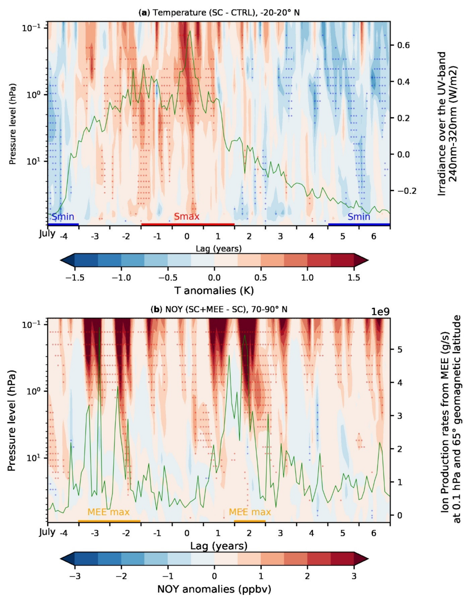
3.1. Forcing from UV Irradiance and MEE

We begin by demonstrating that, in the equatorial middle atmosphere, temperatures are modulated by the UV irradiance variability throughout the solar cycle. In Figure 1a, the equatorial monthly-mean, ensemble-mean temperature differences between the SC and CTRL experiments (herefafter, SC-CTRL) in the stratosphere and lower mesosphere are displayed along with the applied radiative flux anomalies over the UV-band spanning 230–340 nm. In the rest of this paper, the time along the x-axis is indicated as lagged years with respect to the solar maximum (lag zero), the year when the main peak of the UV radiative flux occurred. The red horizontal lines delineate the three years that will be later composited as the part of the broad solar maximum conditions (hereafter referred to as lags −1, 0, and 1) and the blue lines the corresponding three solar minimum years (hereafter referred to as lags −4, 5, and 6), hereafter collectively called Smax and Smin, respectively. Temperatures are increasing across the lower mesosphere and the mid- and upper stratosphere in the rising part of the solar cycle, culminating in the Smax while progressively decreasing during Smin. These temperature differences are most pronounced at the altitudes of the ozone UV heating but, in certain years, anomalous temperatures are extending downwards into the lower stratosphere, particularly in Smax. The magnitudes of the stratopause temperature anomalies are comparable to those in [35].
We now consider the main effect of the MEE precipitation, which is to generate additional odd nitrogen (NOY) at high latitudes compared to a simulation including only auroral precipitation. To this end, Figure 1b shows the corresponding NOY differences between the two experiments with and without the MEE forcing (hereafter SCMEE-SC). Note that, unlike Figure 1a, the average is taken over the 70°–90° N latitude band to emphasize the polar descent of the NOY produced by EPP in the auroral ovals. To highlight the periods of enhanced MEE forcing in relation to the solar cycle, we have also shown the MEE-induced ion pair production rates, revealing two groups of years with elevated values, one in the rising phase of the solar cycle (lags −4 to −2) and one with the highest values in the declining phase (lags 1 to 2). Except for late parts of lagged year 1, the MEE forcing is weak during Smax and Smin. We see that the wintertime descent brings down elevated positive anomalies of NOY following periods of strong MEE precipitation. Figure S2 shows the NOY abundance throughout the solar cycle at 1 hPa in November, January, and March. NOY is enhanced throughout the cold season in certain years, and on the basis of this figure, we define the years −3, −2, and 2 as the MEE maximum years, hereafter called MEEmax years. We also note from Figure 1b that there is some amount of NOY inter-annual variability, reflecting varying dynamical conditions favoring a pronounced descent.
Since it was shown in Figure 1b that MEE has little impact during Smax or Smin, the two experiments with solar forcing (SC and SCMEE) are amalgamated, i.e., combined and considered as one experiment to double the ensemble size, when we consider the UV irradiance effect.

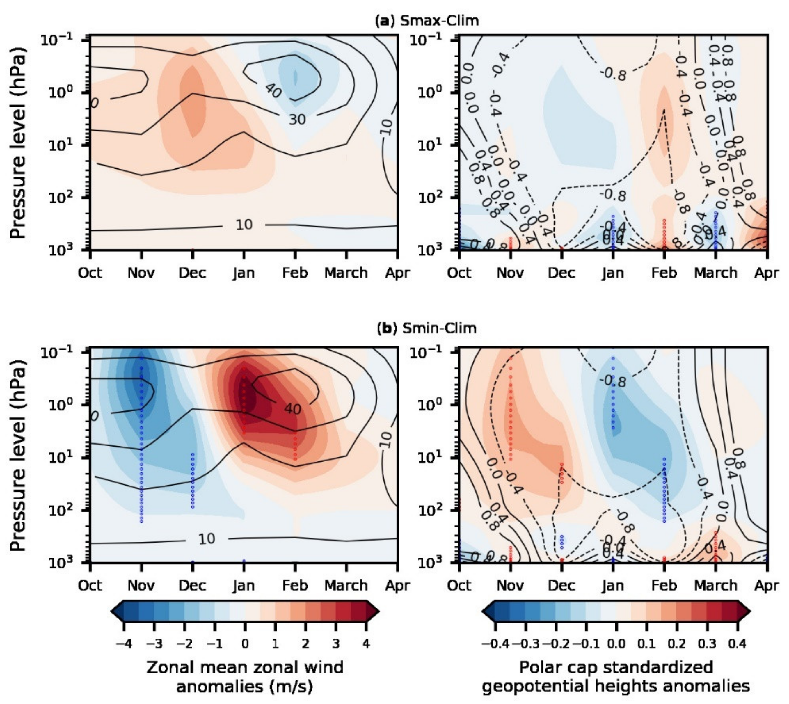
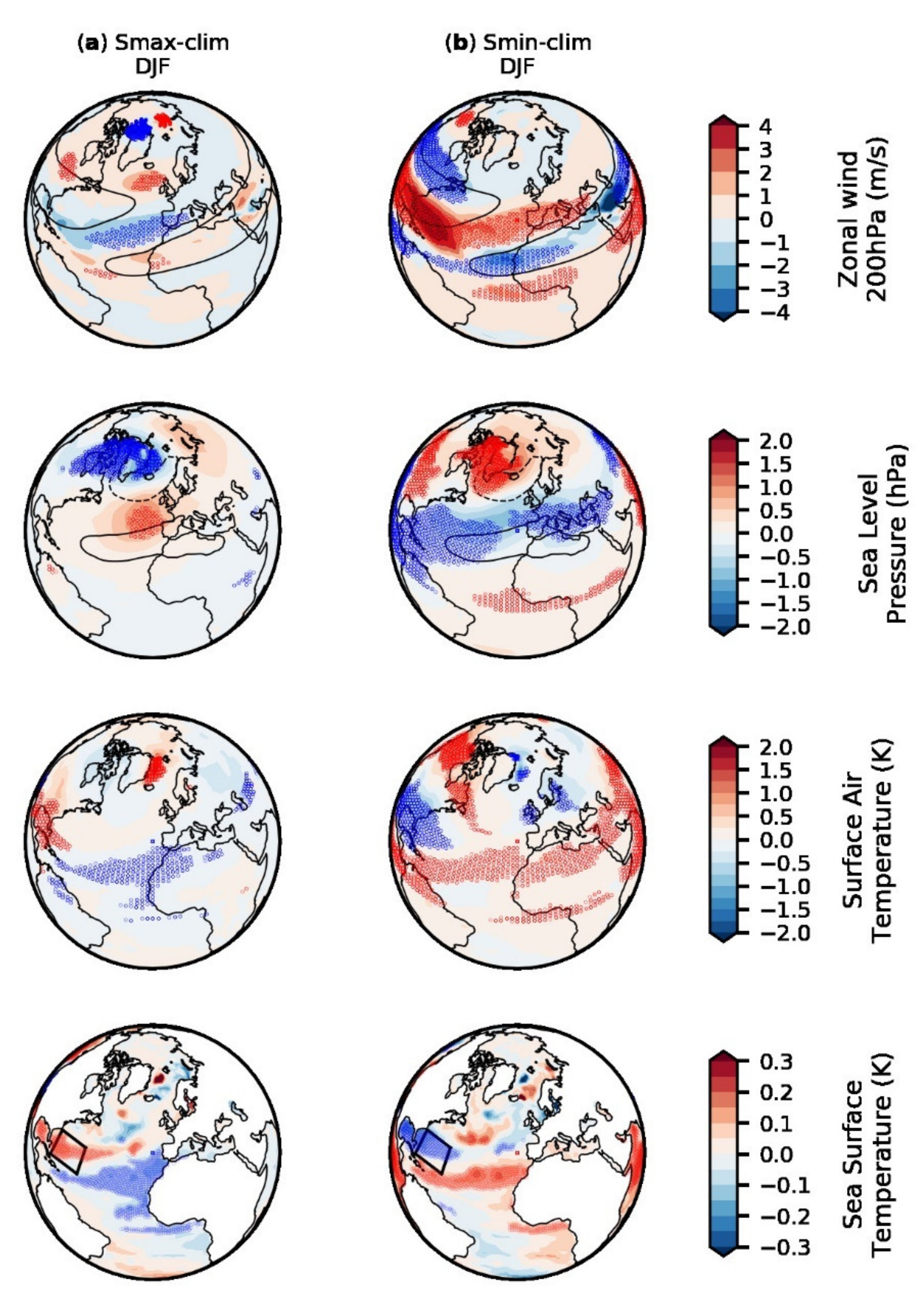
3.2. Stratospheric, Tropospheric, and Surface Effects from UV Irradiance
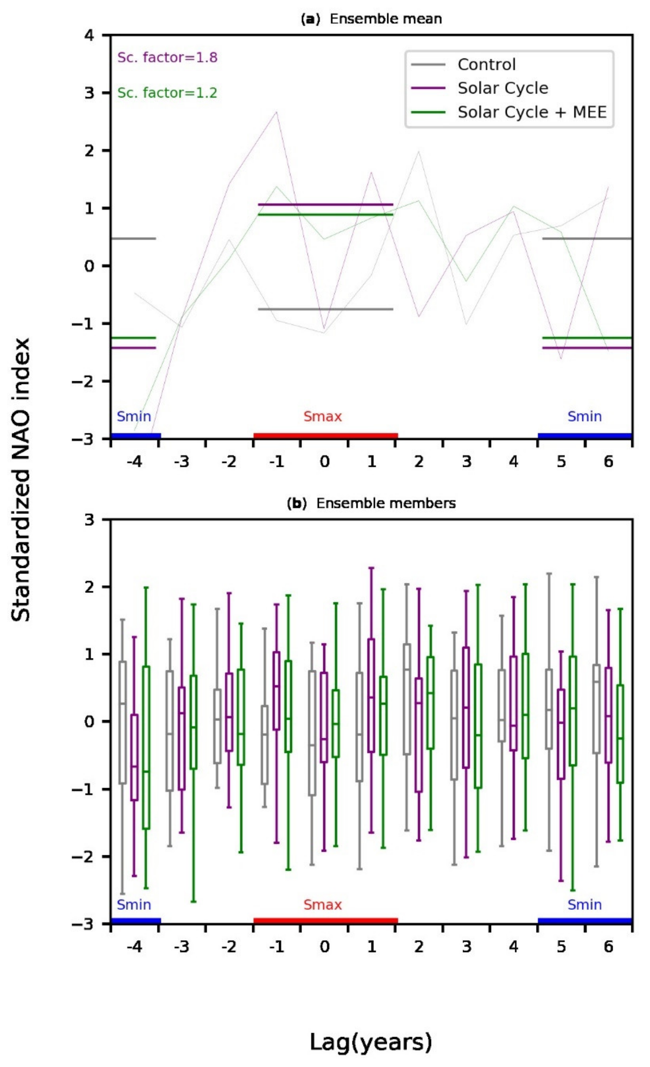
Previous studies (e.g., [7]) suggest that solar irradiance forcing leads to a stronger latitudinal gradient between the polar and the equator during Smax and a weaker gradient during Smin. To investigate to what extent the variations in UV irradiance strengthens or weakens the polar vortex, we show in Figure 2 the seasonal cycle of the anomalies in zonal-mean zonal wind and the polar cap averaged geopotential heights for the Smax and the Smin. The stratospheric wind anomalies were weak, consistent with other studies on the weak top-down mechanism (e.g., [6,29]) and mostly significant during Smin (zonal winds reaching −3 m/s). In the stratosphere, the model zonal wind anomalies are consistent with the model anomalies in geopotential height, reflecting geostrophic balance.
The preceding analysis seems to indicate that the stratospheric polar vortex is modulated by the solar phase. We now explore how these solar-induced zonal wind anomalies affect the tropospheric jet stream and the surface climate through an inter-annual modulation of the NAO. In Figure 3a,b, we show maps of DJF zonal wind at 200 hPa, SLP, surface air temperature (SAT), and sea surface temperature (SST) anomalies for Smax in (a) and Smin in (b). For comparison, Figure S3 shows the characteristic NAO signature in the same variables, obtained from regression upon the NAO index in the last 50 years of the background run.
We infer from Figure 3 that during DJF the UV irradiance response over the North Atlantic involves a poleward shift of the Atlantic eddy-driven jet in Smax, with a strengthening north of the jet core and a weakening to the south, and an opposite response in Smin. The SLP composites are consistent with the North Atlantic jet shift, with a general weakening (strengthening) of pressure over the Arctic centered over Greenland and a belt of pressure increase (decrease) at mid-latitudes over the North Atlantic in Smax (Smin), stretching from the American East coast into Europe. The Smin anomalies for both SLP and SAT compare well with the characteristic NAO pattern in Figure S3, except that for Smax the zonal extension of the low-pressure region was less pronounced and the northern part of the quadrupole signature in SAT was too weak. This negative NAO-like quadrupole pattern prominent during Smin impacts the meteorological conditions over the European and North American continents. Northern Europe becomes colder and drier, while Southern Europe is associated with milder and wetter winter climate conditions. The opposite occurs over North America, i.e., warmer and wetter in the north and colder and drier in the south. For SST, the solar-induced anomalies bear resemblance to the characteristic tripole SST pattern associated to the NAO (see Figure S3d for the NAO positive phase): the southern lobe with cooling in Smax and warming in Smin is similarly positioned off the coast of West Africa, but the middle lobe of the tripole, characterized by warming in Smax and cooling in Smin, is situated slightly to the south of the characteristic NAO middle lobe. Similarly, the northern lobe of the tripole, with cooling in Smax and warming in Smin, is shifted southward compared to the NAO northern lobe. A strong point to confirm the solar origin of the aforementioned NAO signatures is the absence of characteristic NAO signatures in the corresponding figure for CTRL (Figure S4), using the exact same years during which there is no difference in solar forcing.

3.3. The NAO Index

Prediction systems have a deterministic NAO index variance much smaller than found in observations requiring a scaling up for comparison (e.g., [20]) and at the same time a high member-to-member NAO variability. Consequently, observations, ensemble-means, and ensemble members are often separately standardized relative to their respective standard deviations [19,21]. We begin with ensemble-means by presenting standardized, ensemble-mean NAO index time series to unravel the role of solar forcing. Here, we are comparing different experiments with different forcings, and hence we adopted a scaling approach to display the NAO time series after they have been standardized for each of the three experiments (see Appendix B for details). The standardized time series are scaled by a factor that is the ratio of the forced experiment ensemble-mean variance to the corresponding variance of the CTRL experiment. Hence, the NAO time series for the CTRL experiment is truly standardized (the scaling factor is one), while the scaled NAO timeseries of the twin forced experiments (not truly standardized since the variance is not one anymore) reveal the extent to which the NAO index variability is changed with respect to the CTRL. The scaling factors being larger than 1 indicate that the variance is higher in the forced experiments. In fact, it was almost doubled for SC (the scaling factor is 1.8).
The DJF time series of the scaled NAO indices are shown in Figure 4a for the ensemble means of the three experiments. In both forced experiments, the NAO index is substantially stronger in Smax than in Smin when averaged over the three Smax and Smin years and, relative to the CTRL experiment, more positive in Smax and more negative in Smin. This confirms the positive NAO patterns in DJF SLP in Figure 3 for Smax and vice versa for Smin.
Figure 4b represents the corresponding NAO indices for all ensemble members presented as boxplots. Here, the ensemble members have been standardized to their standard deviation (see Appendix B), and it is apparent that the member-to-member variability is very high in any year. Even if the medians of the ensemble (horizontal lines in boxplots) deviate among experiments, they remain between the first and third quartile of each other boxplots, indicating that differences between the experiments are not likely to be significantly different. The same applies to interannual differences within each experiment. To further investigate the strength of the forced DJF NAO signal, we estimated the signal-to-noise (S/N) ratios. Following the common practice in prediction systems, S/N is the ratio of the ensemble-mean (or external) interannual variance to the internal (e.g., inter-member and interannual) variance. The S/N values are listed in Table 2 for each forced experiment (SC and SCMEE) and for their amalgamation (SC + SCMEE). The key point is that the S/N ratios are all very small (e.g., 0.03 for the amalgamated experiment), indicating the dominance of internal variability. However, such small S/N ratios are commonly found in coupled dynamical prediction systems: for example, [20] found a S/N ratio of 0.09 for the Artic Oscillation seasonal forecast.
The calculated spatial distribution of the S/N ratios for SLP from the amalgamated experiment in DJF (Figure 5) revealed that while the Arctic, North Atlantic, and the North Pacific (although the latter is not emphasized here) were the regions associated with the largest variability, the forced signal expanded west of the North Atlantic region of high variability. The S/N ratio was also found to be enhanced in the subtropics. In other words, the UV irradiance signal did not perfectly project onto the NAO. We note again that the S/N ratios were very small, an important result indicating the overwhelming predominance of the model internal variability over the response to external forcing.

3.4. Stratospheric, Tropospheric, and Surface Effects from UV Irradiance

It has been suggested that SST anomalies forced by solar variability can reemerge from one year to the next and amplify atmosphere–ocean interactions over several years, ultimately causing the NAO to peak a few years after solar maximum [8,9]. In these studies, the reemergence mechanism was suggested to operate mostly in the middle lobe of the characteristic NAO SST tripole pattern. The 3-year Smax ensemble-mean composite (Figure 3a) also indicates a pronounced SST increase off the coast of Florida and northern Caribbean, i.e., in a region slightly to the south of the characteristic NAO middle lobe (compare NAO SST anomalies in Figure S4d to the position of the black square).
To provide an indication of a weak reemergence in our simulations, Figure 6a shows the ocean temperature anomalies in this region (black square in Figure 3 and Figure S4d). In accordance with the reemergence mechanism, a significant warming was observed, synchronized with the solar maximum, starting first within the deep wintertime mixed-layer, and later sheltered beneath the shallower summertime mixed-layer. In other words, warm SST anomalies in wintertime induced by the top-down solar forcing survive beneath the mixed-layer during summer and then reemerge at the sea surface in the following winter. As the top-down forcing endures during the Smax years, the surface signal is amplified, reaching its maximum during the last Smax year. There is also evidence for surface cooling during the Smin years. The fact that this synchronized reemergence is associated with the solar cycle was further supported by the corresponding ocean temperature anomalies for the CTRL simulation (Figure S5): warm season anomalies above the shallow thermocline were found, but at lags 4 and 5, and hence not synchronized with the solar maximum.
We found in Figure 3a,b that the SST anomalies were located slightly south of the middle lobe of the characteristic NAO tripole pattern. Although Figure 6a shows a reemergence of SST anomalies synchronized with solar maximum, it is situated in a region far south of the oceanic fronts, which are the key regions of ocean–atmosphere interaction, especially in winter [14,15]. To demonstrate this further, we show in Figure 6b a latitude-depth cross-section of ocean temperatures during three boreal summer–fall periods (JJASON) and winter–spring (DJFMAM) in the western Atlantic, averaged over the longitude sector 70°–40° W. The three periods encompass the three years where re-emergence occurred (within the two vertical lines in Figure 6a). A warm anomaly can be seen south of 35° N in the first summer–fall, with high temperature anomalies sequestered at depth below the shallow thermocline. Over the next two summer–fall periods, it intensified (still sequestered at depth) and was moving slightly poleward towards 40° N. In the winter–spring, the warm anomaly extended to the surface and was strongest and most poleward in the last winter. However, these anomalies, despite their northward migration, remained too far south from the surface oceanic fronts characterized by large meridional temperature gradients located around 40° N in winter, as can be inferred from the climatological temperatures (black contours). The temperatures during the respective summer–fall or winter–spring periods (dashed black contours) were nearly identical to the climatology, indicating that there are only very weak changes in the meridional temperature gradient in the frontal zones. We take this as an indication that, while there is a solar signal in the upper ocean, the solar-induced atmosphere–ocean feedback is prevented from occurring, hence a lack of a lagged surface NAO response to the solar cycle.

3.5. Stratospheric, Tropospheric, and Surface Effects from UV Irradiance

In this last section, we investigate whether any dynamical effect in the stratosphere could be related to the NOY enhancements during MEEmax. We show in Figure 7 cross-sections of the zonal-mean zonal winds anomalies from November to March for each individual MEEmax year in the SCMEE experiment. We first note that by comparing the different years, there is no coherent pattern in the seasonal cycle of the zonal wind. We then show in Figure S6 the corresponding anomalous zonal winds in the same 3 years in the CTRL experiment and in Figure S7 for the SC experiment (although there was no MEE forcing in the CTRL or SC experiments). From the examination of these three figures, we find that the large year-to-year differences between the three MEEmax years in SCMEE, the similarities of monthly anomalies among the forced and unforced experiments, and the lack of significance in most months support the notion that the MEE signature is not systematic nor consistent.
There is only one conspicuous case of polar vortex strengthening in SCMEE that is not found in the CTRL or SC experiments. Hence, we surmise that this polar vortex strengthening that occurred in December in lagged year 2, the strongest MEEmax year (see Figure 1b), might be related to MEE forcing. In the same way as was done for the UV irradiance case, we checked whether the stratospheric changes left any characteristic signal in the troposphere. To this end, we show in Figure 8a,b the zonal wind anomalies at 200 hPa in the last MEEmax year (lagged year 2) in December and the corresponding anomalies in SLP in January. We found that there were significant positive zonal wind anomalies on the poleward flank of the climatological Atlantic jet in December, which were consistent with the strengthening of the polar vortex in Figure 7. At the surface, the anomalous SLP manifested as an Arctic low but was not significant. Hence, it appears unlikely that the MEE forcing led to any significant changes in the NAO, albeit the significant stratospheric jet strengthening in December of lagged year 2 was consistent with the results of the atmosphere-only WACCM simulations with MEE in [32].

4. Discussion

To further elucidate whether the combined effects of the UV irradiance variations and EPP (more specifically MEE precipitation) throughout the 11-year solar cycle had a notable impact on the North Atlantic winter climate and ocean-atmosphere interactions over the North Atlantic Ocean, we focused on solar cycle 23 in an idealized framework. While the solar forcings were realistic, other forcings such as the QBO, GHGs, and large volcanic eruptions were either excluded or held constant. Solar proton events have also been neglected. We used a configuration of NorCPM, wherein a high-top chemistry-climate model (WACCM) was coupled to an isopycnic coordinate ocean model (MICOM). In addition to the radiative forcing, prescribed as for CMIP6, we included realistic MEE forcing. We carried out three experiments, with 25 ensemble members each, for present-day climate conditions. To extract possible UV irradiance signals on stratospheric and tropospheric climate, we compared three-year averages of solar max and solar min conditions with the climatology. To investigate the extent of MEE impacts, we considered three years diagnosed with the highest ion production rates and odd nitrogen amounts. Our ensemble decadal simulations focused on the solar cycle 23 and hence differed from other comparable studies with WACCM [6,16], which consisted of multi-centennial simulations with repeated sequences of 4–5 different solar cycles. A key novelty of our investigation is the detailed investigation of the ocean–atmosphere coupling related to the solar signal in the North Atlantic, carried out for the first time with a high-top chemistry-climate model such as WACCM.
Our results show that, in Smax (Smin), the strengthened (weakened) polar vortex anomalies reached down into the troposphere. The downward migration of zonal-mean zonal wind anomalies linked to the UV irradiance variability compare qualitatively with existing results (e.g., [1,16,24,29]), with a weak top-down mechanism. As a consequence of the zonal wind increase in solar max years, the North Atlantic part of the jet stream was shifted poleward, and the surface climate response projected onto a NAO positive phase.
The Aleutian Low variability exerts a strong influence on the polar stratospheric vortex variability. Through its influence on the Aleutian Low variability, the PDO (Pacific Decadal Oscillation) strongly modulates the amplitude of the solar UV irradiance effects [3]. The strengthened stratospheric polar vortex during Smax is more pronounced during the PDO negative phase, through anomalous meridional advection of solar-induced temperature anomalies, which contributes to lessen the meridional eddy heat flux. This PDO modulation of the stratosphere vortex might well exert a downward influence on the Atlantic sector too in our simulations. Such inter-basin coupling will be examined in further work.
Our calculated NAO indices for DJF showed a positive NAO anomaly in Smax years and a negative NAO anomaly in Smin years, when compared with the CTRL constant-forcing simulations. Our results support the idea of a NAO response to the solar cycle forcing, albeit the surface pressure and temperature responses slightly deviate from the classical NAO pattern. Other studies have argued that atmosphere–ocean interactions allow for an amplification of the NAO response during solar max through reemerging SSTs, resulting in the strongest NAO impact 2–4 years after solar maximum [8,9,14]. Other model studies did not find a lagged response [2]. Although we found evidence of re-emergence of SST, we did not find such a lagged impact on the NAO. Since the model main ocean temperature response was situated in a region equatorward of the middle lobe of the NAO tripole and did not migrate northward to the Atlantic Ocean frontal region, local air–sea interaction in winter was prevented, thus contributing to a weaker NAO response. This plausibly explains the absence of a multi-year lagged NAO atmospheric response to solar forcing, despite the presence of the solar signal in the upper Atlantic Ocean. The efficacy of the re-emergence mechanism to trigger an atmospheric NAO response to solar forcing might therefore be model-dependent, and perhaps also dependent on the atmospheric and oceanic resolution. Further comparative multi-model studies are certainly warranted.
Despite showing a robust NOY increase during the MEEmax years, our analysis reveals that the MEE forcing is not associated to a systematic response. There are no coherent stratospheric zonal-mean zonal wind changes in the ensemble mean during the three MEEmax years. Comparing the SCMEE simulations to the SC and CTRL simulations, we only found a strengthening of the polar vortex in December during the last MEEmax year, which appeared consistent with previous studies [32,38], but significant tropospheric effects were not present. This is also supported by Figure 4a, where no positive anomaly in ensemble-mean NAO indices is found for the combined MEEmax years. In summary, despite the realistic MEE forcing dataset used in this study, the resulting excess of NOY in the MEEmax years (which was quite apparent at 1 hPa, see Figure S2) did not lead to a significant, consistent dynamical signal in the stratosphere amidst the large internal atmospheric variability. It is nevertheless a possibility that abrupt changes in MEE activity, at sub-monthly scales, linked to distinct strong events, might cause dynamical effects that are hidden in our monthly output or manifests only in given years. Further studies of extreme precipitation events are warranted to elucidate that point.
Through calculations of S/N ratios, our study demonstrates that the forced signals are in fact very weak compared to the internal variability of the ocean–atmosphere system. These results are in line with recent studies (e.g., [49,50]) suggesting that climate prediction models respond too little to external forcings (e.g., volcanic, solar, or ozone) and that their internal variability is too high, so that models have difficulty in reproducing themselves. In climate prediction systems, the large model spread requires large ensemble runs to demonstrate deterministic prediction skill of the NAO [51]. These studies further indicated that this so-called “signal-to-noise paradox” manifests strongly over the North Atlantic sector where the NAO might be susceptible to such external forcings and more predictable in the real world [50]. In particular, the very low S/Ns for the NAO index in our forced experiments (Table 2) indicate that both UV irradiance and MEE forcings induces a low potential predictability (the ratio of the external to the total, internal plus external, variance, that can be inferred from Table 2). Nevertheless, this does not preclude that solar forcing could play a role in forcing the NAO and that improving its representation might improve the skill of a coupled prediction system despite the low S/N ratio [52]. The phase of the QBO is known to influence the variability of the polar vortex and to condition the middle atmosphere response to external forcings; hence, further studies on the role of the QBO are warranted. Additionally, our results are affected by the evolution from the initial ocean state. Further studies on the combined effects from UV irradiance (and MEE) during a solar cycle should therefore cover a broad range of initial ocean conditions to reveal any dependence of the solar response to the ocean mean state.

Supplementary Materials

The following are available online at https://www.mdpi.com/article/10.3390/atmos12081029/s1, Figure S1: The multi-decadal evolution of the ocean temperatures in the background run and the spread of the ensemble members initialized from year 50. Figure S2: NOY mixing ratios over the solar cycle for three different months (November, January and March) at 1hPa. Figure S3: Correlation between the standardized DJF NAO index (the principal component of the 1st EOF) and the anomalies of the DJF for zonal winds at 200 hPa (m/s), sea level pressure (hPa), surface air temperature (K) and sea surface temperatures (K). Figure S4: Anomalies (in filled contours) as in Figure 3, but for the CTRL. Figure S5: Anomalies as in Figure 6a, but for the CTRL. Figure S6: Anomalies as in Figure 7, but for the CTRL. Figure S7: Anomalies as in Figure 7, but for the SC.

Author Contributions

Conceptualization, S.G., Y.O., F.S., O.H.O., and N.T.; methodology, S.G., Y.O., O.H.O., P.T.V., C.J.R., and M.A.C.; software, S.G. and O.H.O.; formal analysis, S.G.; investigation, S.G., Y.O., F.S., O.H.O., and N.T.; resources, O.H.O., P.T.V., M.A.C., and C.J.R.; data curation, S.G.; writing—original draft preparation, S.G. and Y.O.; visualization, S.G.; supervision, Y.O., F.S., and N.-E.O. All authors have read and agreed to the published version of the manuscript.

Funding

S.G., Y.O., F.S., O.H.O., N.-E.O., and N.T. have been funded by the Norwegian Research Council through project 255276 (Solar effects on natural climate variability in the North Atlantic and Arctic). The work of P.T.V. is supported by the Academy of Finland (project no. 335555 ICT-SUNVAC).

Institutional Review Board Statement

Not Applicable.

Informed Consent Statement

Not Applicable.

Data Availability Statement

Not Applicable.

Acknowledgments

P.T.V., M.A.C., and C.J.R. would like to thank the International Space Science Institute, Bern, Switzerland, for supporting the project “Quantifying Hemispheric Differences in Particle Forcing Effects on Stratospheric Ozone” (leader: D. R. Marsh).

Conflicts of Interest

The authors declare no conflict of interest.

Appendix A

The MEE forcing dataset used in the current study is an updated version of the ISSI-14 energetic electron precipitation data. Appendix A of [31] contains a detailed description of the data processing undertaken to produce that forcing data. In this appendix, we only summarize the earlier approach and note the updates. We direct the interested reader to [31] (Appendix A) for the complete description.
The MEE forcing data relies on experimental measurements by the Medium Energy Proton and Electron Detector (MEPED) carried onboard the NOAA- and MetOp-series of low-earth orbiting satellites, operated by the National Oceanic and Atmospheric Administration and European Organization for the Exploitation of Meteorological Satellites, respectively. We restricted ourselves to MEPED measurements from the SEM-2 (Space Environment Monitor 2) package, first launched onboard NOAA-15 in mid-1998. Over time 5 NOAA and 3 MetOp spacecraft have made measurements with SEM-2, and at times as many as 6 operational SEM-2 carrying spacecraft have been orbiting simultaneously. In the ISSI energetic electron precipitation data, all operational POES measurements are zonally averaged in geomagnetic coordinates, combining both magnetic hemispheres. A 3-h time resolution and 0.5 L resolution is applied, focused primarily on the 45–72 geomagnetic latitude (McIlwain L shell 2–10) range of the outer radiation belts. Combining observations from the three electron telescopes observing electron precipitation, we determined the magnitude and a fitted energy spectra of the precipitation, assuming a power-law energy spectral form from 30-keV to 1 MeV. In both ISSI-approaches, care was taken to avoid auroral proton contamination on the MEPED electron fluxes, the impact of SPE on the satellite measurements, and the loss of quality data in the region of the South Atlantic Magnetic Anomaly. The primary differences in the MEPED data processing between ISSI-14 and ISSI-19 came from improvements in our understanding of LEO electron flux measurements (e.g., [53,54]), changes to allow more modern spacecraft data to be ingested (allowing for format changes) and also corrections in the code used to undertake the auroral proton contamination correction.
Note that we refer to this dataset as “ISSI-19”, building on the earlier “ISSI-14” electron precipitation dataset. Both electron precipitation datasets were then used to determine ionization rate calculations, leading to the ISSI-14 and ISSI-19 MEE forcing approach. ISSI-14 was named as such because the fundamental processing approach used to produce the dataset was originally undertaken during an International Space Science Institute (ISSI) International Team (“Quantifying Hemispheric Differences in Particle Forcing Effects on Stratospheric Ozone”. Leader: D. R. Marsh) in April–May 2014. The new ISSI-19 approach came from discussions during a CHAMOS (Chemical Aeronomy in the Mesosphere and Ozone in the Stratosphere) EEP workshop held in Helsinki in April 2019 (http://chamos.fmi.fi, accessed on 1 April 2021).
The MEE electron observations produced in the ISSI-14 approach formed the basis of the ApEEP MEE electron forcing model, recommended for use in CMIP6 [35]. The ApEEP model was specifically designed for long-term climate runs spanning outside of time periods when satellite precipitation measurements exist. In their study validating the APEEP model forcing, [55] recommended using EEP from direct POES measurements during time periods when such observations exist, and as applied here through ISSI-19. To allow for easy use of the ISSI-19 ionization rates in atmosphere and climate simulations, they were prepared consistent with the ApEEP dataset. In other words, the electron energy range, the atmospheric ionization rate calculation method [56], and the data format are identical to those used in CMIP6.

Appendix B

To extract the solar forcing of the NAO amidst the large internal variability, we first standardized the ensemble-means NAO temporal time series separately from the ensemble members. In other words, the forced, external components represented by the ensemble means were compared between themselves [19,21]. For each experiment ensemble mean, we define a standardized NAO index:
N A O t e x p r = x t e x p r μ e x p r σ e x p r
where x t e x p r is the projected NAO time series and μ e x p r and σ e x p r are the mean and standard deviation of x t e x p r , respectively, whereas t represents the time through the solar cycle and e x p r the experiment (either CTRL, SC or SCMEE).
To compare the change in variance between the forced and the control experiments, we rescaled N A O t e x p r :
N A O t e x p r = N A O t e x p r α
where the scaling factor α is
α = σ e x p r σ c t r l
In that fashion, the N A O t e x p r time series for the CTRL experiment remains truly standardized, while the N A O t e x p r time series of the twin forced experiments reveal the extent to which the NAO index variance was enhanced with respect to the CTRL experiment.
To complement the analysis of the ensemble-means, we followed the exact same procedure with each ensemble members. Then, the standardized NAO indices for the ensembles members were
N A O t , i e x p r = x t , i e x p r μ i e x p r σ i e x p r
where x t , i e x p r is the projected NAO time series for each ensemble member and μ i e x p r and σ i e x p r are the mean and standard deviation of x t , i e x p r , respectively, and i represents each ensemble member (i = 1.25).
The rescaled NAO index is
N A O t , i e x p r = N A O t , i e x p r α
where the scaling factors α is
α = σ e x p r σ c t r l
σ e x p r is then the total temporal and inter-member standard deviation for each experiment. It is important to note that, in order for the forced (or external) components of the variability amidst the large internal variability to be examined, the ensemble-mean time series of each experiment is standardized separately from the ensemble of all members. For each ensemble experiment, external variance σ e x p r 2 (or signal) measures the time variance of the ensemble means across the solar cycle, whereas the internal variance σ e x p r 2 (or noise) measures the temporal and inter-member variance among all the ensemble members. Their ratio is the signal-to-noise ratio (S/N). In addition to the S/N ratio of the NAO index, we similarly define a local (e.g., at every grid point) S/N ratio for the SLP.

References

  1. Gray, L.J.; Beer, J.; Geller, M.; Haigh, J.D.; Lockwood, M.; Matthes, K.; Cubash, U.; Fleitmann, D.; Harrison, G.; Hood, L.; et al. Solar Influences on Climate. Rev. Geophys. 2010, 48. [Google Scholar] [CrossRef]
  2. Gray, L.J.; Scaife, A.A.; Mitchell, D.M.; Osprey, S.; Ineson, S.; Hardiman, S.; Butchart, N.; Knight, J.; Sutton, R.; Kodera, K. A lagged response to the 11 year solar cycle in observed winter Atlantic/European weather patterns. J. Geophys. Res. Atmos. 2013, 118, 420. [Google Scholar] [CrossRef] [Green Version]
  3. Guttu, S.; Orsolini, Y.; Stordal, F.; Otter, O.H.; Omrani, N.E. The 11 year solar cycle UV irradiance effect and its dependency on the Pacific Decadal Oscillation. Environ. Res. Lett. 2021, 16. [Google Scholar] [CrossRef]
  4. Chen, H.; Ma, H.; Li, X.; Sun, S. Solar influences on spatial patterns of Eurasian winter temperature and atmospheric general circulation anomalies. J. Geophys. Res. Atmos. 2015, 120, 8642–8657. [Google Scholar] [CrossRef] [Green Version]
  5. Ma, H.; Chen, H.; Gray, L.; Zhou, L.; Li, X.; Wang, R.; Zhu, S. Changing response of the North Atlantic/European winter climate to the 11 year solar cycle. Environ. Res. Lett. 2018, 13. [Google Scholar] [CrossRef]
  6. Chiodo, G.; Oehrlein, J.; Polvani, L.M.; Fyfe, J.C.; Smith, A.K. Insignificant influence of the 11-year solar cycle on the North Atlantic Oscillation. Nat. Geosci. 2019, 12, 94–99. [Google Scholar] [CrossRef]
  7. Kodera, K.; Kuroda, Y. Dynamical response to the solar cycle. J. Geophys. Res. Atmos. 2002, 107, 1–12. [Google Scholar] [CrossRef] [Green Version]
  8. Scaife, A.A.; Ineson, S.; Knight, J.R.; Gray, L.; Kodera, K.; Smith, D.M. A mechanism for lagged North Atlantic climate response to solar variability. Geophys. Res. Lett. 2013, 40, 434–439. [Google Scholar] [CrossRef]
  9. Andrews, M.B.; Knight, J.R.; Gray, L.J. A simulated lagged response of the North Atlantic Oscillation to the solar cycle over the period 1960–2009. Environ. Res. Lett. 2015, 10. [Google Scholar] [CrossRef] [Green Version]
  10. Visbeck, M.; Chassignet, E.P.; Curry, R.G.; Delworth, T.L.; Dickson, R.R.; Krahmann, G. The ocean’s response to North Atlantic oscillation variability. Geophys. Monograph Am. Geophys. Union Washington 2003, 134, 113–146. [Google Scholar] [CrossRef] [Green Version]
  11. Taws, S.L.; Marsh, R.; Wells, N.C.; Hirschi, J. Re-emerging ocean temperature anomalies in late-2010 associated with a repeat negative NAO. Geophys. Res. Lett. 2011, 38, 1–6. [Google Scholar] [CrossRef] [Green Version]
  12. Yukimoto, S.; Kodera, K. Annular modes forced from the stratosphere and interactions with the oceans. J. Meteorol. Soc. Jpn. 2007, 85, 943–952. [Google Scholar] [CrossRef] [Green Version]
  13. Gray, L.J.; Woollings, T.J.; Andrews, M.; Knight, J. Eleven-year solar cycle signal in the NAO and Atlantic/European blocking. Q. J. R. Meteorol. Soc. 2016, 142, 1890–1903. [Google Scholar] [CrossRef] [Green Version]
  14. Yukimoto, S.; Kodera, K.; Thiéblemont, R. Delayed North Atlantic response to solar forcing of the stratospheric polar vortex. Sci. Online Lett. Atmos. 2017, 13, 53–58. [Google Scholar] [CrossRef] [Green Version]
  15. Omrani, N.E.; Ogawa, F.; Nakamura, H.; Keenlyside, N.; Lubis, S.W.; Matthes, K. Key Role of the Ocean Western Boundary currents in shaping the Northern Hemisphere climate. Sci. Rep. 2019, 9, 1–12. [Google Scholar] [CrossRef] [PubMed]
  16. Thiéblemont, R.; Matthes, K.; Omrani, N.E.; Kodera, K.; Hansen, F. Solar forcing synchronizes decadal North Atlantic climate variability. Nat. Commun. 2015, 6, 1–8. [Google Scholar] [CrossRef] [PubMed] [Green Version]
  17. Otterå, O.H.; Bentsen, M.; Drange, H.; Suo, L. External forcing as a metronome for Atlantic multidecadal variability. Nat. Geosci. 2010, 3, 688–694. [Google Scholar] [CrossRef]
  18. Cohen, J.; Screen, J.A.; Furtado, J.C.; Barlow, M.; Whittleston, D.; Coumou, D.; Francis, J.; Dethloff, K.; Entekhabi, D.; Overland, J.; et al. Recent Arctic amplification and extreme mid-latitude weather. Nat. Geosci. 2014, 7, 627–637. [Google Scholar] [CrossRef] [Green Version]
  19. Orsolini, Y.J.; Senan, R.; Vitart, F.; Balsamo, G.; Weisheimer, A.; Doblas-Reyes, F.J. Influence of the Eurasian snow on the negative North Atlantic Oscillation in subseasonal forecasts of the cold winter 2009/2010. Clim. Dyn. 2016. [Google Scholar] [CrossRef] [Green Version]
  20. Stockdale, T.N.; Molteni, F.; Ferranti, L. Atmospheric initial conditions and the predictability of the Arctic Oscillation. Geophys. Res. Lett. 2015, 42, 1173–1179. [Google Scholar] [CrossRef]
  21. Scaife, A.A.; Arribas, A.; Blockley, E.; Brookshaw, A.; Clark, R.T.; Dunstone, N.; Eade, R.; Fereday, D.; Folland, C.K.; Gordon, M.; et al. Skillful long-range prediction of European and North American winters. Geophys. Res. Lett. 2014. [Google Scholar] [CrossRef] [Green Version]
  22. Honda, M.; Yamane, S.; Nakamura, H. Impacts of the Aleutian-Icelandic low seasaw on surface climate during the twentieth century. J. Clim. 2005, 18, 2793–2802. [Google Scholar] [CrossRef]
  23. Li, F.; Orsolini, Y.J.; Wang, H.; Gao, Y.; He, S. Modulation of the Aleutian–Icelandic low seesaw and its surface impacts by the Atlantic Multidecadal Oscillation. Adv. Atmos. Sci. 2018. [Google Scholar] [CrossRef] [Green Version]
  24. Mitchell, D.M.; Misios, S.; Gray, L.J.; Tourpali, K.; Matthes, K.; Hood, L.; Schmidt, H.; Chiodo, G.; Thiéblemont, R.; Rozanov, E.; et al. Solar signals in CMIP-5 simulations: The stratospheric pathway. Q. J. R. Meteorol. Soc. 2015, 141, 2390–2403. [Google Scholar] [CrossRef] [Green Version]
  25. Misios, S.; Mitchell, D.M.; Gray, L.J.; Tourpali, K.; Matthes, K.; Hood, L.; Schmidt, H.; Chiodo, G.; Thiéblemont, R.; Rozanov, E.; et al. Solar signals in CMIP-5 simulations: Effects of atmosphere-ocean coupling. Q. J. R. Meteorol. Soc. 2015, 142, 928–941. [Google Scholar] [CrossRef]
  26. Ineson, S.; Scaife, A.A.; Knight, J.R.; Manners, J.C.; Dunstone, N.J.; Gray, L.J.; Haigh, J.D. Solar forcing of winter climate variability in the Northern Hemisphere. Nat. Geosci. 2011, 4, 753–757. [Google Scholar] [CrossRef] [Green Version]
  27. Lean, J.L.; DeLand, M.T. How does the Sun’s spectrum vary? J. Clim. 2012, 25, 2555–2560. [Google Scholar] [CrossRef]
  28. Cullens, C.Y.; England, S.L.; Garcia, R. The 11 year solar cycle signature on wave-driven dynamics in WACCM. J. Geophys. Res. Sp. Phys. 2016, 121, 3484–3496. [Google Scholar] [CrossRef] [Green Version]
  29. Tartaglione, N.; Toniazzo, T.; Orsolini, Y.; Otterå, O.H. Impact of solar irradiance and geomagnetic activity on polar NOx, ozone and temperature in WACCM simulations. J. Atmos. Sol.-Terr. Phys. 2020, 209, 105398. [Google Scholar] [CrossRef]
  30. Andersson, M.E.; Verronen, P.T.; Marsh, D.R.; Seppälä, A.; Päivärinta, S.M.; Rodger, C.J.; Clilverd, M.A.; Kalakoski, N.D.; Van De Kamp, M. Polar Ozone Response to Energetic Particle Precipitation Over Decadal Time Scales: The Role of Medium-Energy Electrons. J. Geophys. Res. Atmos. 2018, 123, 607–622. [Google Scholar] [CrossRef]
  31. Orsolini, Y.J.; Smith-Johnsen, C.; Marsh, D.R.; Stordal, F.; Rodger, C.J.; Verronen, P.T.; Clilverd, M.A. Mesospheric Nitric Acid Enhancements During Energetic Electron Precipitation Events Simulated by WACCM-D. J. Geophys. Res. Atmos. 2018. [Google Scholar] [CrossRef] [Green Version]
  32. Guttu, S.; Orsolini, Y.; Stordal, F.; Limpasuvan, V.; Marsh, D.R. WACCM simulations: Decadal winter-to-spring climate impact on middle atmosphere and troposphere from medium energy electron precipitation. J. Atmos. Sol.-Terr. Phys. 2020, 209, 105382. [Google Scholar] [CrossRef]
  33. Rozanov, E.; Calisto, M.; Egorova, T.; Peter, T.; Schmutz, W. Influence of the Precipitating Energetic Particles on Atmospheric Chemistry and Climate. Surv. Geophys. 2012, 33, 483–501. [Google Scholar] [CrossRef] [Green Version]
  34. Sinnhuber, M.; Funke, B. Energetic electron precipitation into the atmosphere. In The Dynamic Loss of Earth’s Radiation Belts; Jaynes, A., Usanova, M., Eds.; Elsevier: Amsterdam, The Netherlands, 2020; pp. 279–321. [Google Scholar]
  35. Matthes, K.; Funke, B.; Andersson, M.E.; Barnard, L.; Beer, J.; Charbonneau, P.; Clilverd, M.A.; Dudok De Wit, T.; Haberreiter, M.; Hendry, A.; et al. Solar forcing for CMIP6 (v3.2). Geosci. Model Dev. 2017. [Google Scholar] [CrossRef] [Green Version]
  36. Seppälä, A.; Lu, H.; Clilverd, M.A.; Rodger, C.J. Geomagnetic activity signatures in wintertime stratosphere wind, temperature, and wave response. J. Geophys. Res. Atmos. 2013, 118, 2169–2183. [Google Scholar] [CrossRef] [Green Version]
  37. He, S.; Wang, H.; Li, F.; Li, H.; Wang, C. Solar-wind-magnetosphere energy influences the interannual variability of the northern-hemispheric winter climate. Natl. Sci. Rev. 2020, 7, 141–148. [Google Scholar] [CrossRef] [Green Version]
  38. Arsenovic, P.; Rozanov, E.; Stenke, A.; Funke, B.; Wissing, J.M.; Mursula, K.; Tummon, F.; Peter, T. The influence of Middle Range Energy Electrons on atmospheric chemistry and regional climate. J. Atmos. Sol.-Terr. Phys. 2016, 149, 180–190. [Google Scholar] [CrossRef] [Green Version]
  39. Li, F.; Orsolini, Y.J.; Keenlyside, N.; Shen, M.L.; Counillon, F.; Wang, Y.G. Impact of Snow Initialization in Subseasonal-to-Seasonal Winter Forecasts with the Norwegian Climate Prediction Model. J. Geophys. Res. Atmos. 2019, 124, 10033–10048. [Google Scholar] [CrossRef] [Green Version]
  40. Bentsen, M.; Bethke, I.; Debernard, J.B.; Iversen, T.; Kirkevåg, A.; Seland, Ø.; Drange, H.; Roelandt, C.; Seierstad, I.A.; Hoose, C.; et al. The Norwegian Earth System Model, NorESM1-M – Part 1: Description and basic evaluation of the physical climate. Geosci. Model Dev. 2013, 6, 687–720. [Google Scholar] [CrossRef] [Green Version]
  41. Marsh, D.R.; Garcia, R.R.; Kinnison, D.E.; Boville, B.A.; Sassi, F.; Solomon, S.C.; Matthes, K. Modeling the whole atmosphere response to solar cycle changes in radiative and geomagnetic forcing. J. Geophys. Res. Atmos. 2007, 112, 1–20. [Google Scholar] [CrossRef] [Green Version]
  42. Neale, R.B.; Gettelman, A.; Park, S.; Chen, C.; Lauritzen, P.H.; Williamson, D.L.; Conley, A.J.; Kinnison, D.; Marsh, D.; Smith, A.K.; et al. Description of the NCAR Community Atmosphere Model (CAM5). NCAR Tech. Note TN-486 2012, 1, 1–12. [Google Scholar]
  43. Bleck, R.; Rooth, C.; Hu, D.; Smith, L.T. Salinity-driven Thermocline Transients in a Wind- and Thermohaline-forced Isopycnic Coordinate Model of the North Atlantic. J. Phys. Oceanogr. 1992, 22, 1486–1505. [Google Scholar] [CrossRef] [Green Version]
  44. Coddington, O.; Lean, J.L.; Pilewskie, P.; Snow, M.; Lindholm, D. A solar irradiance climate data record. Bull. Am. Meteorol. Soc. 2016, 97, 1265–1282. [Google Scholar] [CrossRef]
  45. Yeo, K.L.; Ball, W.T.; Krivova, N.A.; Solanki, S.K.; Unruh, Y.C.; Morrill, J. UV solar irradiance in observations and the NRLSSI and SATIRE-S models Special Section. J. Geophys. Res. Sp. Phys. 2015, 120, 6055–6070. [Google Scholar] [CrossRef]
  46. Wang, Y.-M.; Lean, J.L.; Sheeley, N.R., Jr. Modeling the Sun’s Magnetic Field and Irradiance since 1713. Astrophys. J. 2005, 625, 522–538. [Google Scholar] [CrossRef]
  47. Kay, J.E.; Deser, C.; Phillips, A.; Mai, A.; Hannay, C.; Strand, G.; Arblaster, J.M.; Bates, S.C.; Danabasoglu, G.; Edwards, J.; et al. The community earth system model (CESM) large ensemble project: A community resource for studying climate change in the presence of internal climate variability. Bull. Am. Meteorol. Soc. 2015, 96, 1333–1349. [Google Scholar] [CrossRef] [Green Version]
  48. Espinosa, L.A.; Portela, M.M.; Rodrigues, R. Significant extremal dependence of a daily north atlantic oscillation index (Naoi) and weighted regionalised rainfall in a small island using the extremogram. Water 2020, 12, 2989. [Google Scholar] [CrossRef]
  49. Scaife, A.A.; Smith, D. A signal-to-noise paradox in climate science. NPJ Clim. Atmos. Sci. 2018, 1, 1–8. [Google Scholar] [CrossRef]
  50. Smith, D.M.; Scaife, A.A.; Eade, R.; Athanasiadis, P.; Bellucci, A.; Bethke, I.; Bilbao, R.; Borchert, L.F.; Caron, L.P.; Counillon, F.; et al. North Atlantic climate far more predictable than models imply. Nature 2020, 583, 796–800. [Google Scholar] [CrossRef]
  51. Eade, R.; Smith, D.; Scaife, A.; Wallace, E.; Dunstone, N.; Hermanson, L.; Robinson, N. Do seasonal-to-decadal climate predictions underestimate the predictability of the real world? Geophys. Res. Lett. 2014, 41, 5620–5628. [Google Scholar] [CrossRef]
  52. Dunstone, N.; Smith, D.; Scaife, A.; Hermanson, L.; Eade, R.; Robinson, N.; Andrews, M.; Knight, J. Skilful predictions of the winter North Atlantic Oscillation one year ahead. Nat. Geosci. 2016, 9, 809–814. [Google Scholar] [CrossRef]
  53. Whittaker, I.C.; Gamble, R.J.; Rodger, C.J.; Clilverd, M.A.; Sauvaud, J.A. Determining the spectra of radiation belt electron losses: Fitting DEMETER electron flux observations for typical and storm times. J. Geophys. Res. Sp. Phys. 2013. [Google Scholar] [CrossRef] [Green Version]
  54. Whittaker, I.C.; Rodger, C.J.; Clilverd, M.A.; Sauvaud, J.-A. The effects and correction of the geometric factor for the POES/MEPED electron flux instrument using a multisatellite comparison. J. Geophys. Res. Sp. Phys. 2014, 119, 6386–6404. [Google Scholar] [CrossRef] [Green Version]
  55. Clilverd, M.A.; Rodger, C.J.; van de Kamp, M.; Verronen, P.T. Electron Precipitation from the Outer Radiation Belt During the St. Patrick’s Day Storm 2015: Observations, Modeling, and Validation. J. Geophys. Res. Sp. Phys. 2020, 125, 1–12. [Google Scholar] [CrossRef]
  56. Fang, X.; Randall, C.E.; Lummerzheim, D.; Wang, W.; Lu, G.; Solomon, S.C.; Frahm, R.A. Parameterization of monoenergetic electron impact ionization. Geophys. Res. Lett. 2010. [Google Scholar] [CrossRef]
Figure 1. Monthly zonal-mean anomalies (in filled contours) of (a) temperature (K) in SC-CTRL averaged over latitudes between 20° S–20° N and (b) NOY (N + NO + NO2 +NO3 + 2N2O5 + HNO3 + HO2 NO2 + ORGNOY + NH4NO3, in ppbv) in SCMEE-SC averaged over latitudes between 70° and 90° N. The horizontal axes represent lagged years with respect to solar maximum (years counted from July to July). Colored dots represent locations of statistically significant anomalies. The green solid line indicates in (a) the irradiance forcing integrated over the UV wavelengths (230–340 nm) (Wm−2) and in (b) the ion production rates from MEE precipitation at 0.1 hPa and 65° N geomagnetic latitude. Smax and Smin years are indicated with red and blue horizontal lines along the time axis and the MEE max years with orange lines. Shown are ensemble-mean anomalies.
Atmosphere 12 01029 g001
Figure 2. Annual cycle of monthly zonal-mean zonal wind anomalies at 60° N (m/s, in filled contours) and standardized geopotential heights averaged over latitudes between 60° and 90° N. The anomalies are between Smax and the climatology of the remaining years (Smax excluded) in (a) and between Smin and the climatology of the remaining years (Smin excluded) in (b). We have combined the SC and SCMEE experiments. The geopotential heights are standardized separately at each level. The black contours indicate the respective climatologies. Colored dots represent locations of statistically significant anomalies. Shown are ensemble-mean anomalies.
Atmosphere 12 01029 g002
Figure 3. Anomalies (in filled contours) as in Figure 2 for zonal winds (m/s) at 200 hPa, sea level pressure (hPa), surface air temperature (K), and sea surface temperature (K) for DJF in (a) for Smax-clim and (b) for Smin-clim. In the zonal wind and SLP panels, black contours show the climatological jet and SLP, respectively. The black square indicates the region with high SST. Colored dots represent locations of statistically significant anomalies. Shown are ensemble-mean anomalies.
Atmosphere 12 01029 g003
Figure 4. NAO indices from the three experiments CTRL, SC and SCMEE over the model simulation period for (a) ensemble means in DJF and (b) ensemble members in DJF illustrated as boxplots. The NAO indices are first individually standardized and then scaled. In (a), the scaling involves the standard deviation of the CTRL ensemble mean, implying that CTRL is truly standardized and the scaling factors for SC and SCMEE are indicated. In (b), the scaling involves the overall standard deviation of the CTRL ensemble. The horizontal axis represents lagged years with respect to solar maximum as in Figure 1. Horizontal lines represent the averaged NAO index in the Smax and Smin years.
Atmosphere 12 01029 g004
Figure 5. The total temporal and inter-member variance of SLP over the entire solar cycle in the amalgamated (SC and SCMEE) experiment. This represents the internal variance among 2 × 25 × 11 members. The red contours indicate the local signal-to-noise (S/N) ratios (see Section 2).
Atmosphere 12 01029 g005
Figure 6. (a) Monthly ocean temperature ensemble-mean anomalies (K, in filled contours) between the combined experiments SC and SCMEE and the corresponding annual cycle climatology. The region (70°–40° W, 25°–35° N) in the Atlantic Ocean is indicated by a square in Figure 3a,b. The delineation of the region is based on where significant warm (cold) anomalies close to the middle NAO tripole lobe were detected in Figure 3a,b. The horizontal axis is the same as in Figure 1. The dashed line is the mixed layer depth, representing the seasonally varying thermocline. (b) Meridional cross-sections of corresponding ocean temperature anomalies averaged over 70°–40° W during summer–fall (JJASON) and winter–spring (DJFMAM) are shown for three years lagging the solar peak, between the two black vertical lines in (a). Solid black contours represent the climatological temperatures, while the dashed black contours represent the temperatures in the respective summer–fall or winter–spring periods. The black vertical lines delineate the latitudinal range (25°–35° N) of the region plotted in (a). Colored dots represent locations of statistically significant anomalies. Shown are ensemble-mean anomalies.
Atmosphere 12 01029 g006
Figure 7. Meridional cross-sections of the zonal-mean zonal wind anomalies (m/s) from November to March for the three MEEmax years in SCMEE, (a) Lag – 3, (b) Lag – 2 and (c) Lag + 2. Anomalies are departure from climatology (all years except for the three MEEmax years). Black contours show the climatology. Colored dots represent locations of statistically significant anomalies. Shown are ensemble-mean anomalies.
Atmosphere 12 01029 g007
Figure 8. Anomalies for the last MEEmax year (in experiment SCMEE, in filled contours) for zonal winds (m/s) at 200 hPa in December (a) and sea level pressure (hPa) in January (b). The black contours show the climatological jet or SLP. Colored dots represent locations of statistically significant anomalies. Shown are ensemble-mean anomalies.
Atmosphere 12 01029 g008
Table 1. Overview of simulations, their duration, and number of ensemble members.
SimulationDuration (Years)Ensemble Size
Background run861
CTRL1225
SC1225
SC + MEE1225
Table 2. External variance (signal), internal variance (noise), and the S/N ratios for the NAO index over the entire solar cycle for the SC and SC + MEE experiments and their amalgamation.
Title 1External VarianceInternal VarianceS/N Ratio
SC1.5240.06
SCMEE0.7250.02
SC + SCMEE0.8250.03
Publisher’s Note: MDPI stays neutral with regard to jurisdictional claims in published maps and institutional affiliations.

