
Laser Beam Atmospheric Propagation Modelling for Aerospace LIDAR Applications


Abstract
:1. Introduction
1.1. Aerospace Laser Applications
1.2. Structure of the Article
- Section 2 describes the effects on laser beam performance because of atmospheric attenuation. Covering the Beer–Lambert law governing transmittance, this section introduces the atmosphere composition, the dominant linear propagation effects of absorption and scattering, to then describe the non-linear effects concerning turbulence and thermodynamic propagative effects and the subsequent empirical models and theoretical backgrounds individually.
- Section 3 introduces empirical modelling to collectively combine the propagative effects in terms of laser performance. The benefits of empirical modelling in comparison to atmospheric radiative transfer codes are highlighted, and the approaches are subsequently reflected in practical radiometric measurement techniques for atmospheric extinction.
- Section 4 reviews the main atmospheric radiative transfer codes and emphasizes the underpinning methodology of the line-by-line analysis, the inherent assumptions and applications of each model and identifies trends in model development including more extensive use of absorption and scattering models.
2. Atmospheric Extinction and Transmittance
2.1. Atmospheric Properties
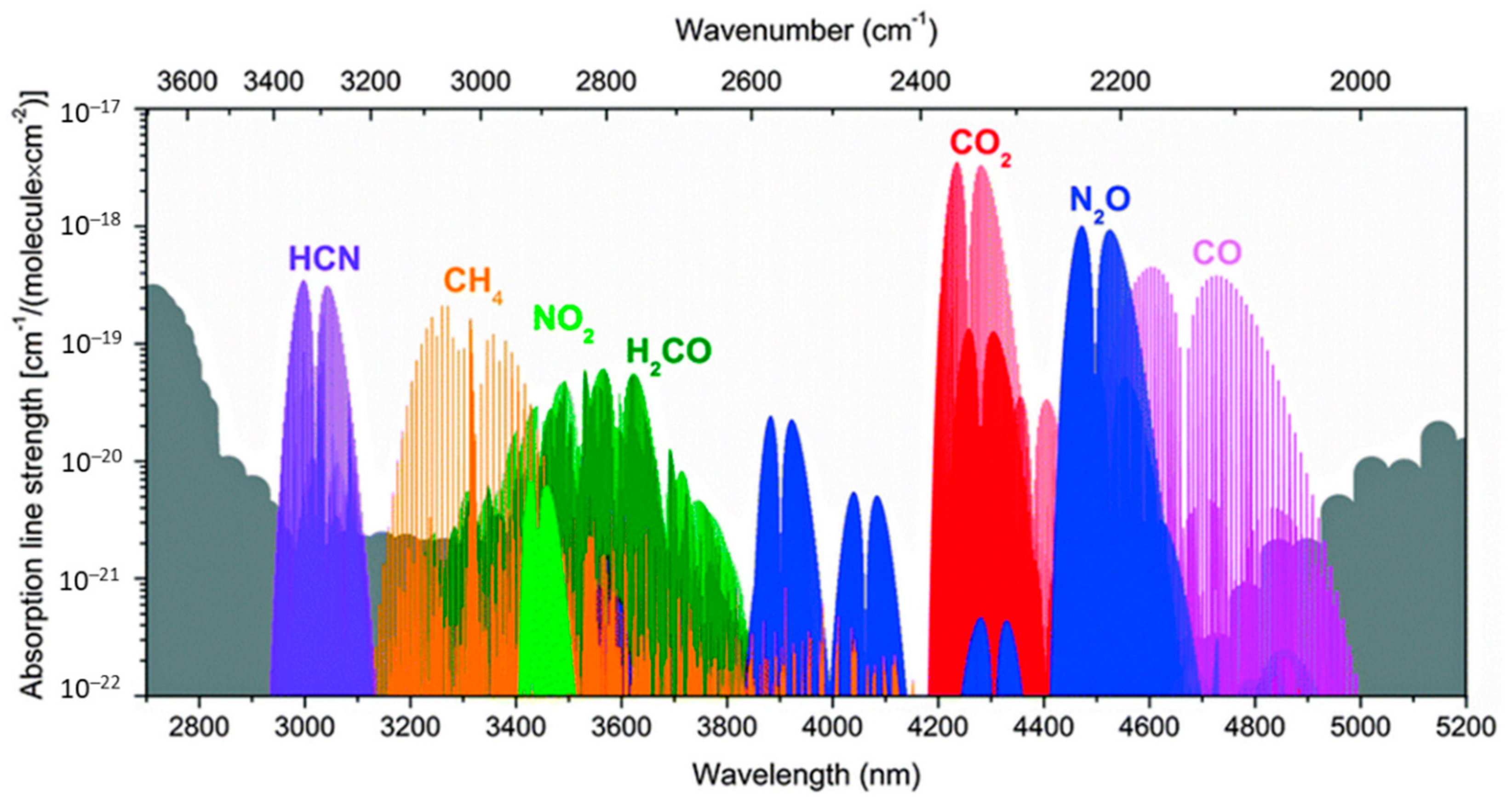
2.2. Molecular Line Absorption
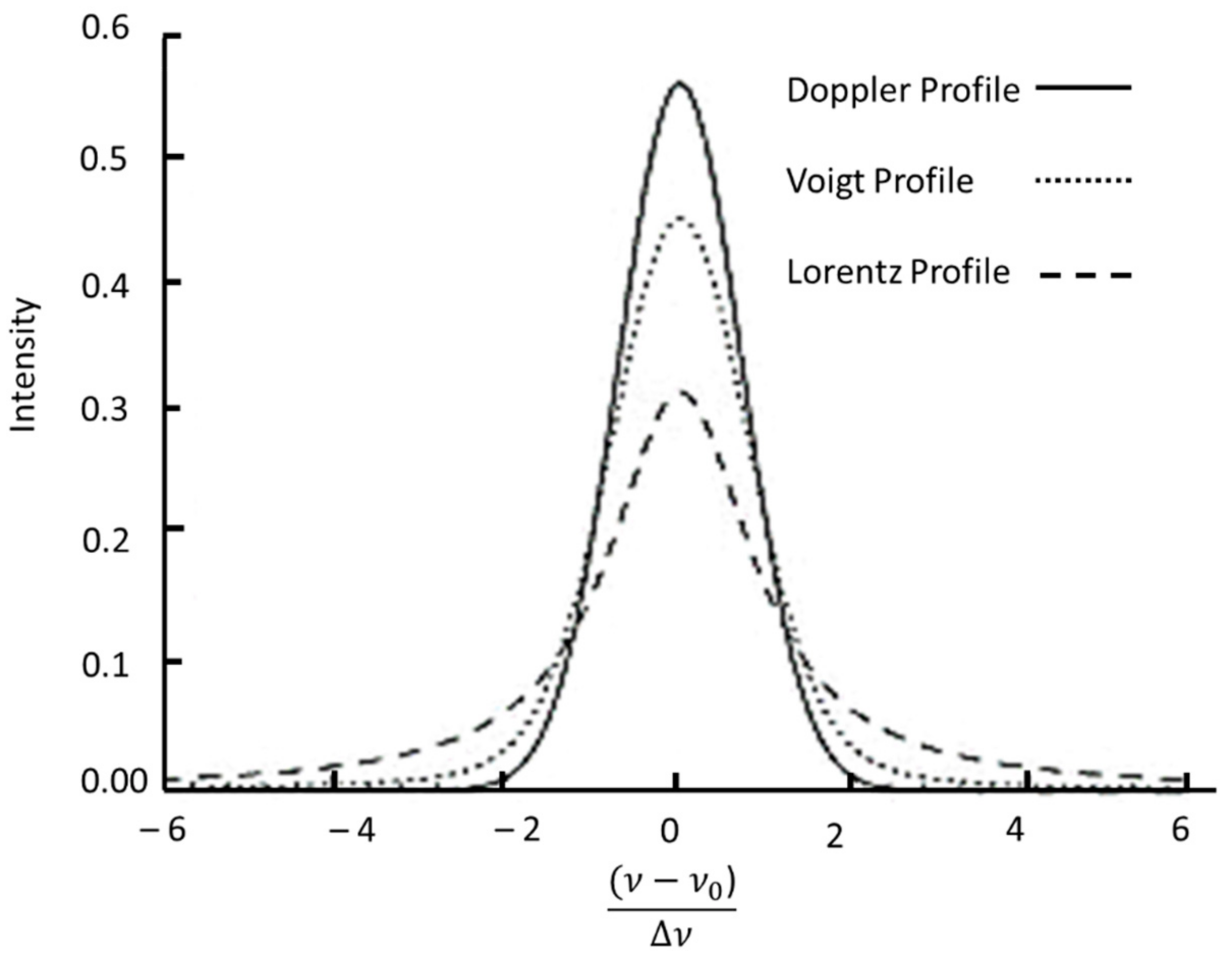
2.2.1. Absorption Line Profile
2.2.2. Continuum Absorption
2.2.3. Transmittance Attenuated by Molecular Line Absorption
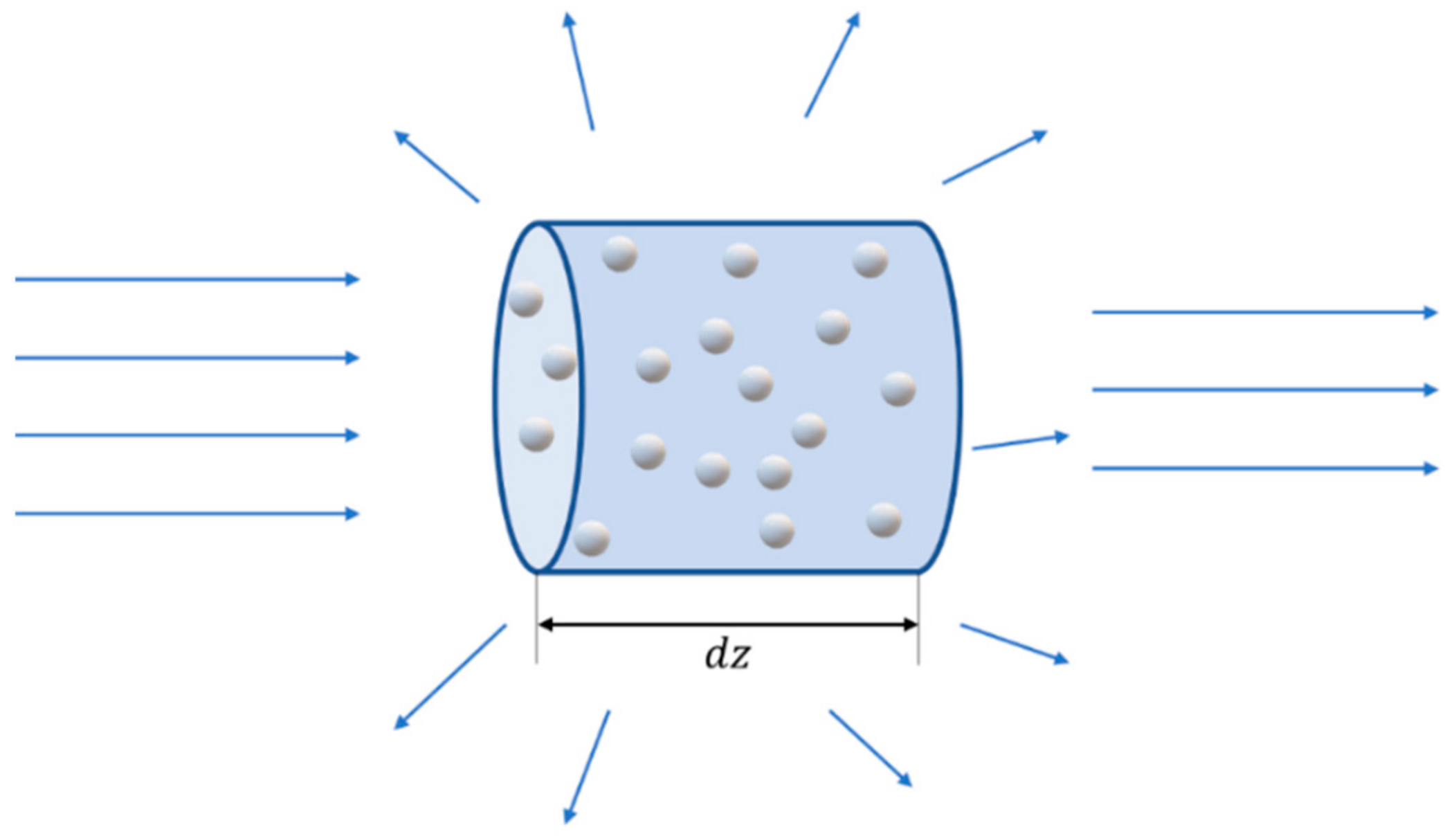
2.3. Atmospheric Scattering
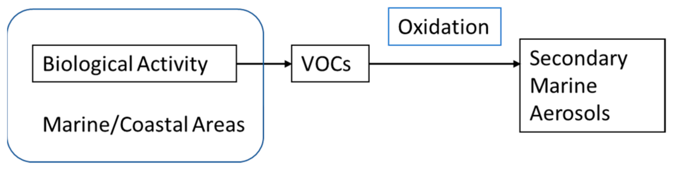
2.3.1. Aerosols
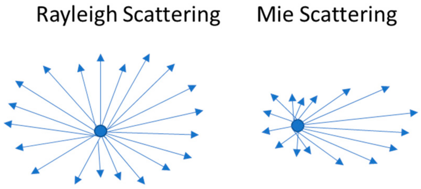
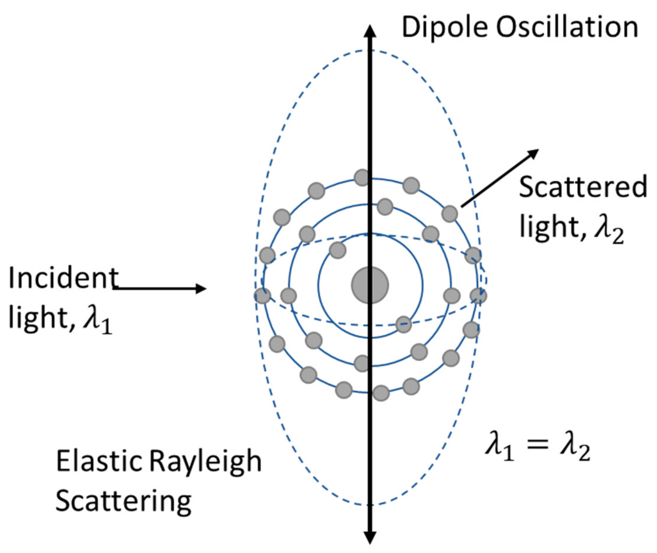
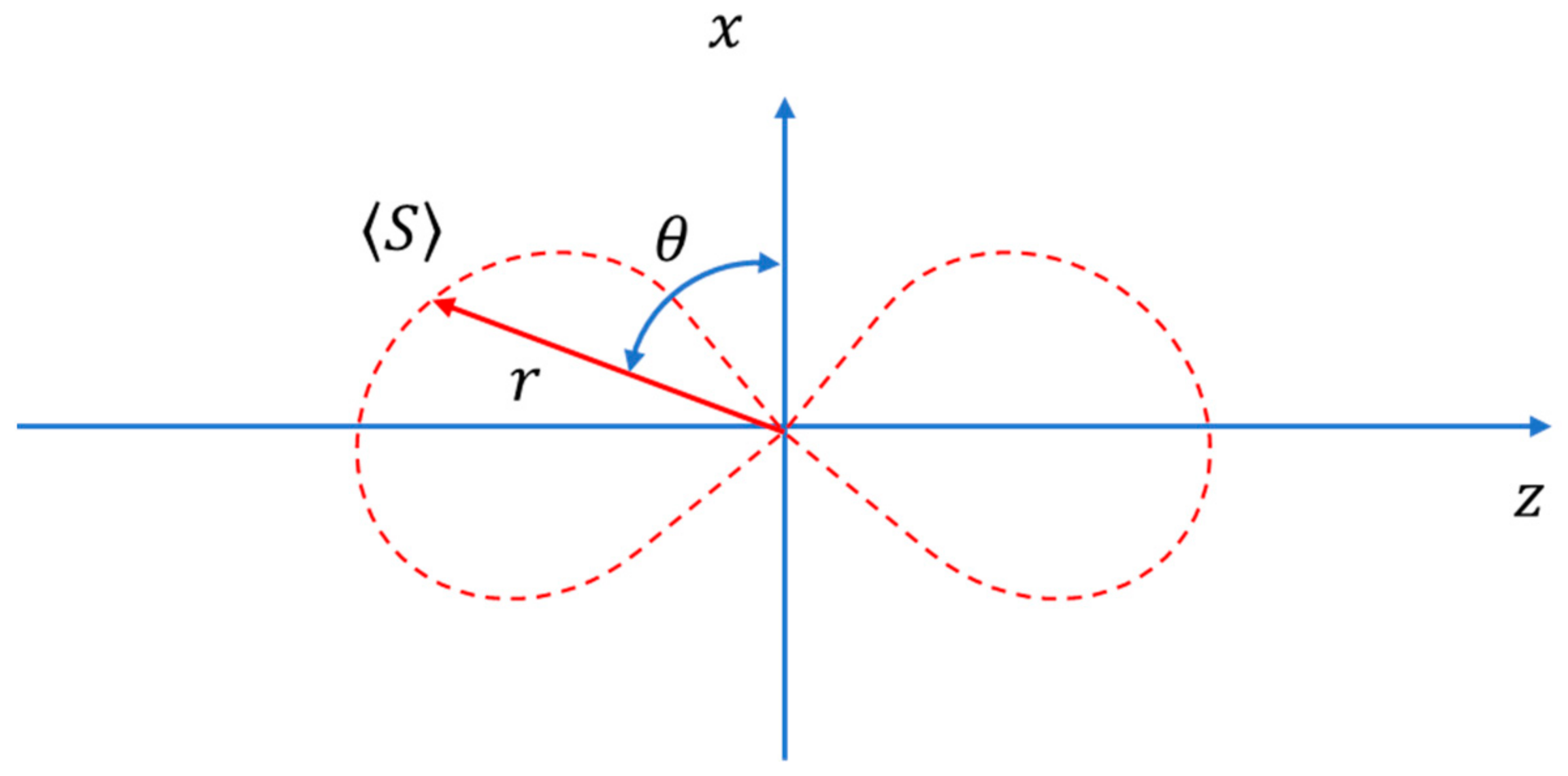
2.3.2. Rayleigh Scattering
2.3.3. Mie Scattering
2.4. Nonlinear Propagation Effects
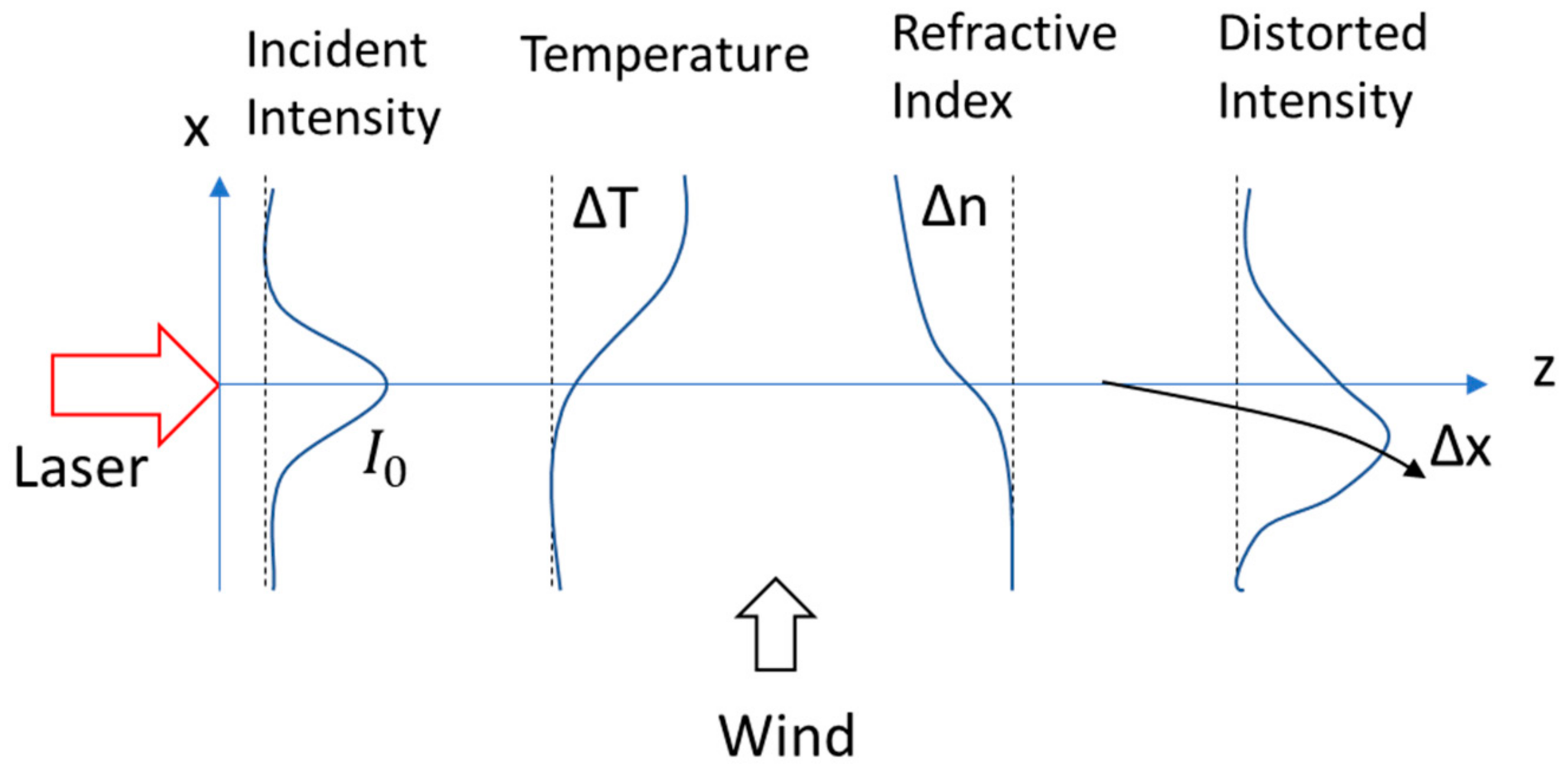
2.4.1. Thermal Blooming
2.4.2. Kinetic Cooling
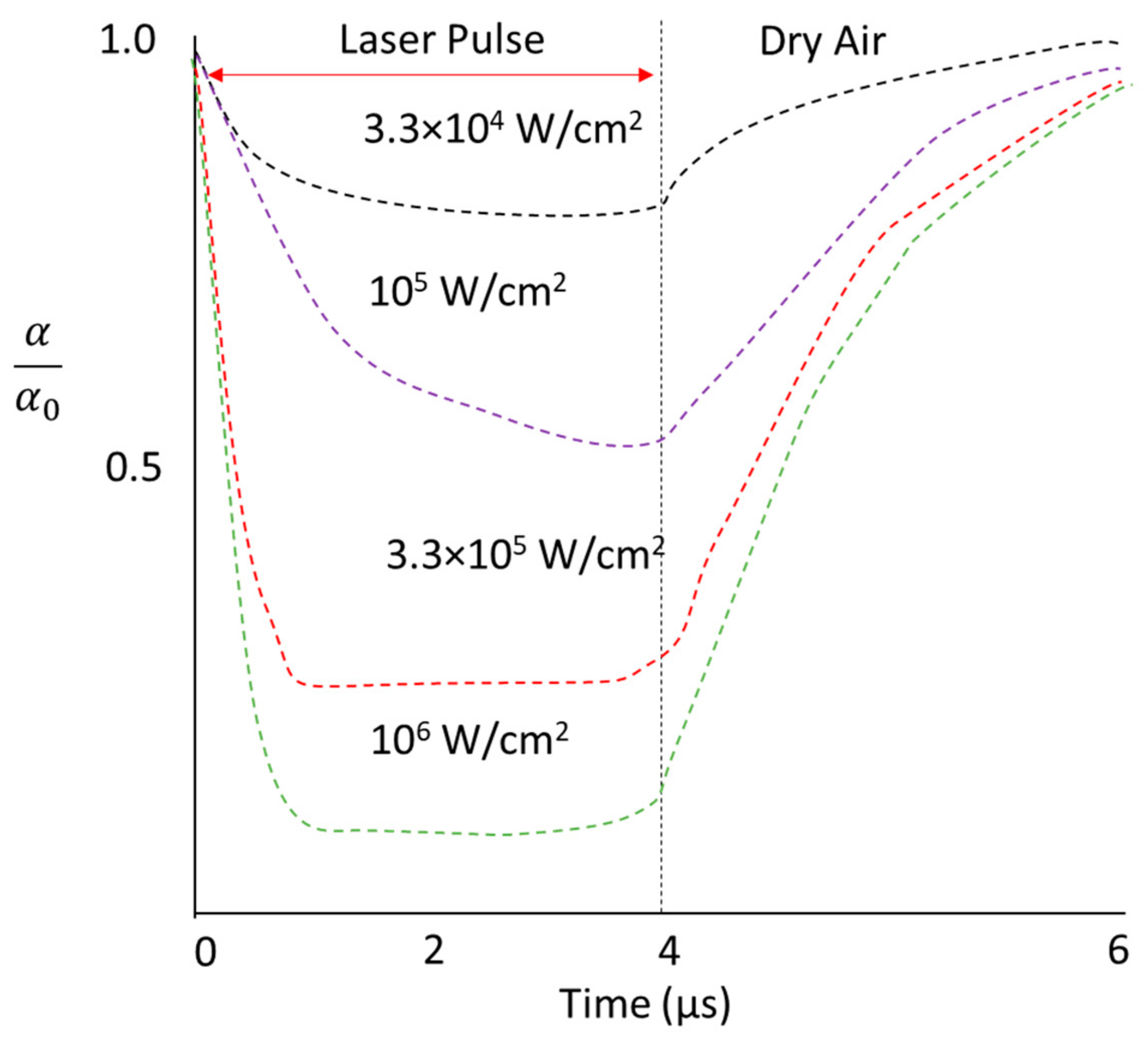
2.4.3. Bleaching
2.4.4. Aerodynamic Effects
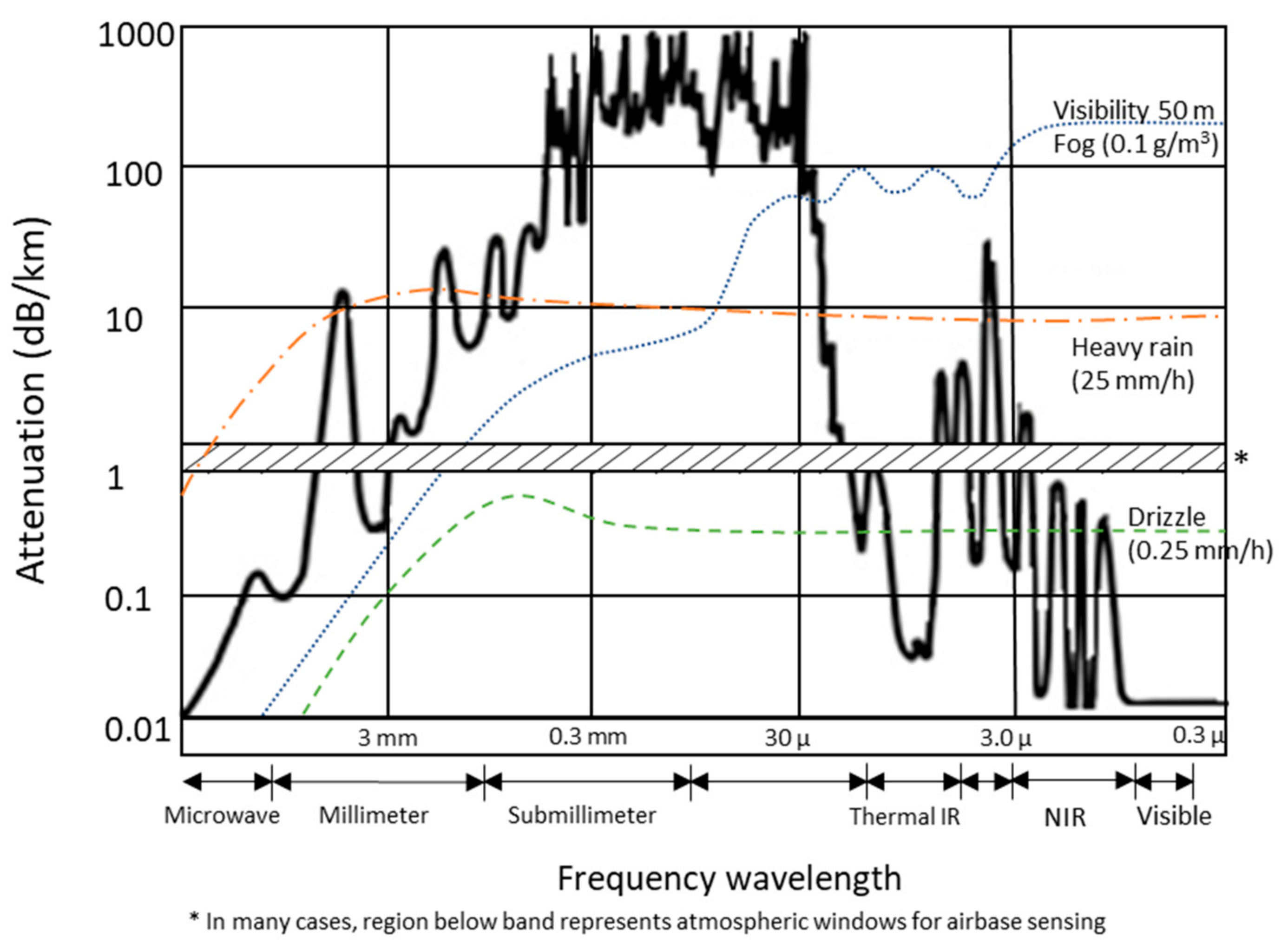
2.5. Propagation through Haze, Fog and Rain
2.6. Propagation through Atmospheric Turbulence
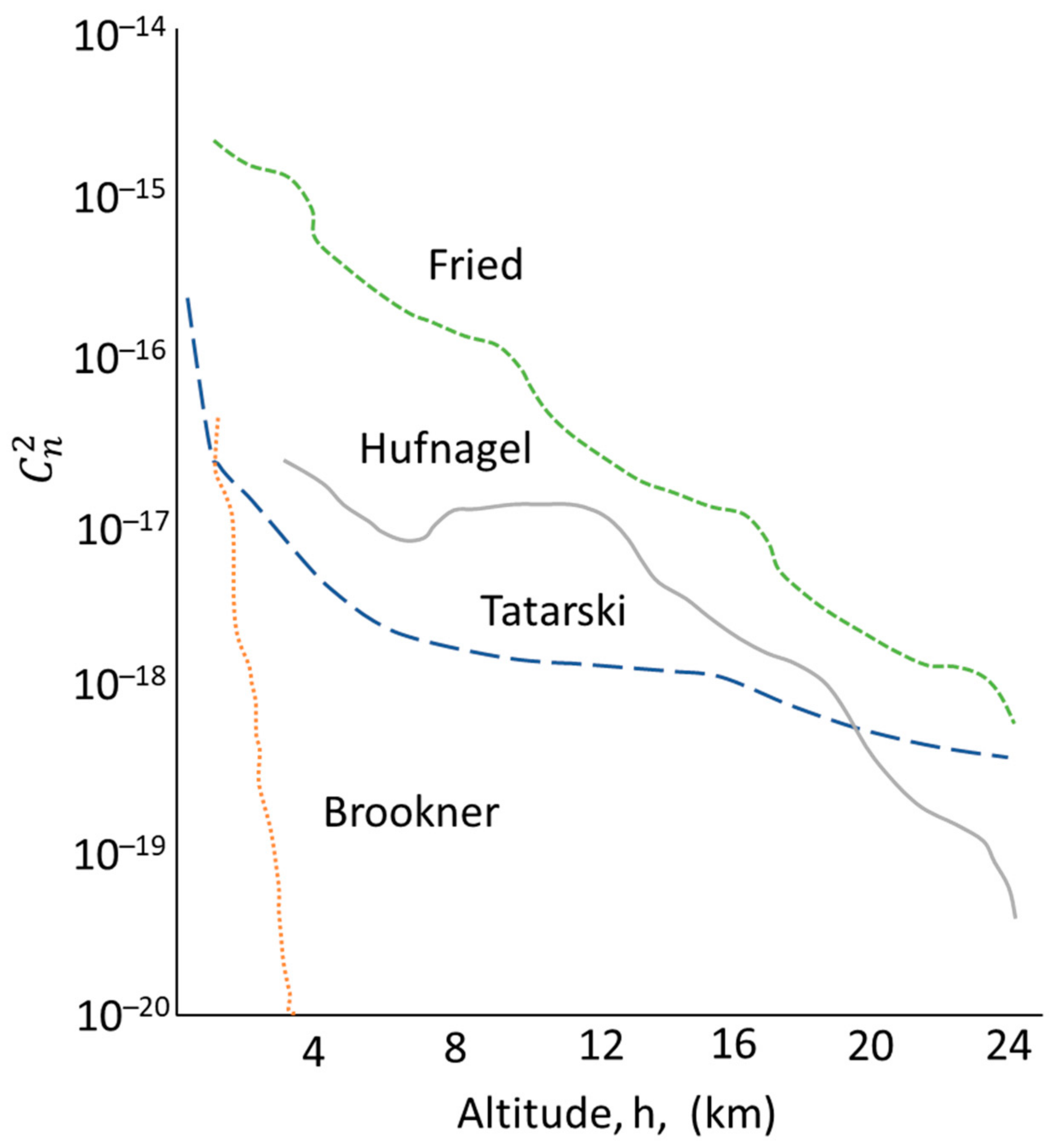
2.6.1. Refractive Index Structure Coefficient

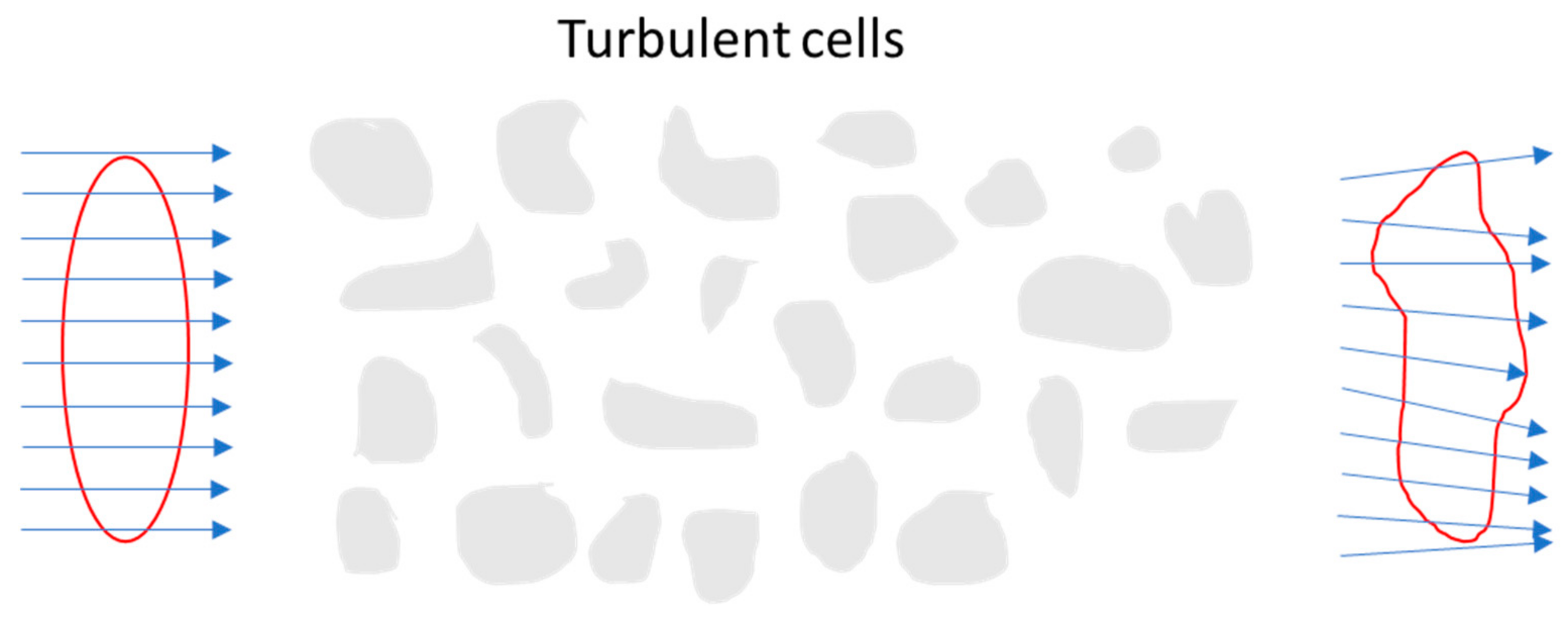
2.6.2. Turbulence Effects
2.6.3. Astronomical Refraction
3. Combined and Empirical Propagation Models
3.1. Laser Range Equation
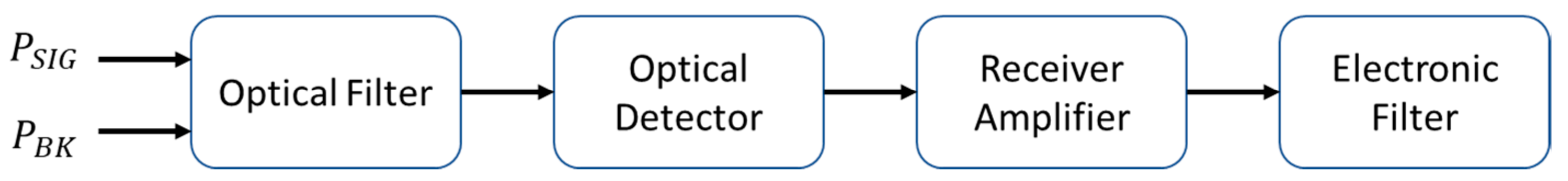
3.2. Signal to Noise Ratio
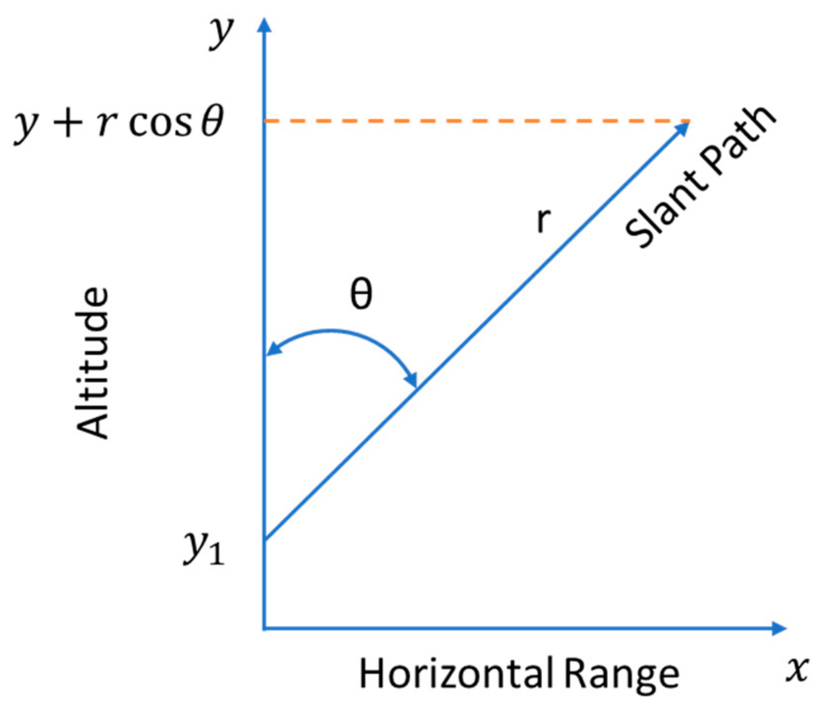
3.3. Laser Beam Transmittance along a Slant Path
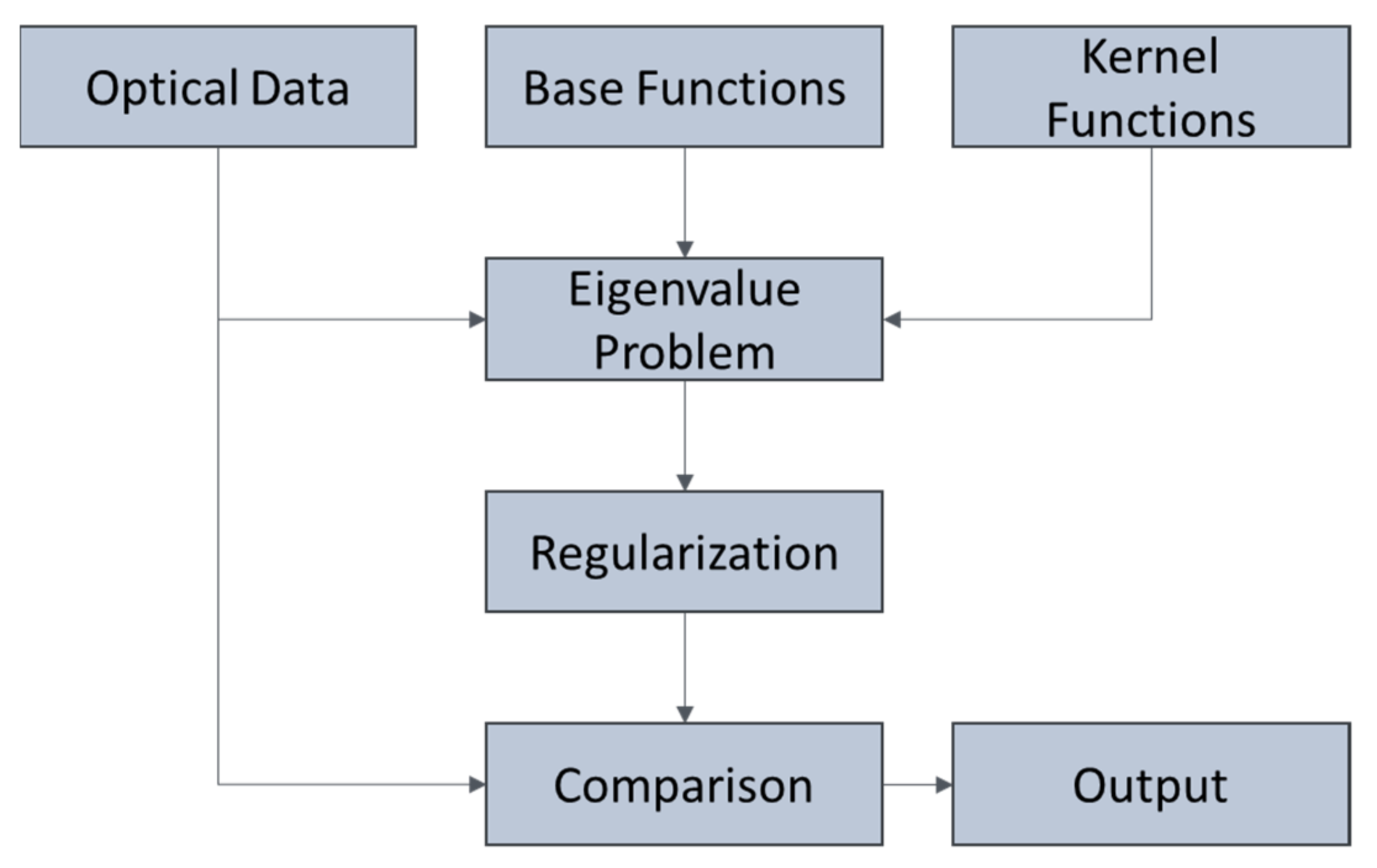
3.4. Particle Retrieval
3.5. Elder–Strong–Langer Model for Absorption
3.6. Elder–Strong–Langer Model for Scattering
3.7. Combined ESLM Model
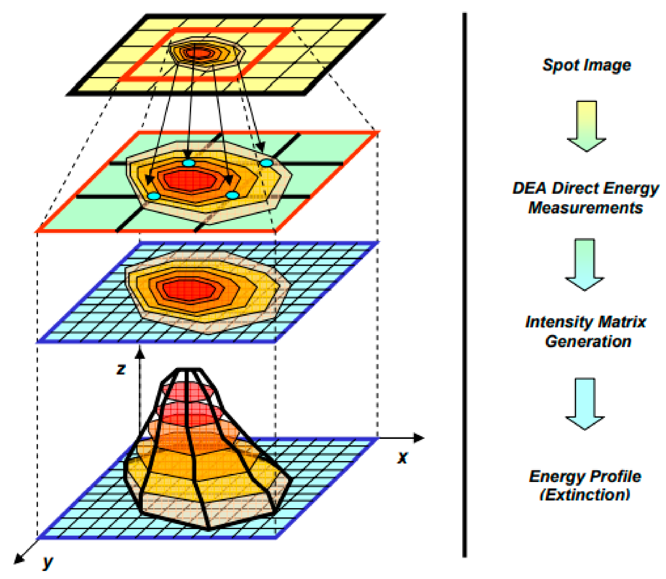
3.8. Radiometric Measurements of Atmosphere Extinction
3.9. Application of Machine Learning in Laser Propagation
4. Atmospheric Radiative Transfer Models
4.1. 4A/OP
4.2. ARTS
4.3. LIDORT/VLIDORT
4.4. 6S/6SV1
4.5. MODTRAN
4.6. LBLRTM
4.7. COART
4.8. DISORT
4.9. MOSART
4.10. RTTOV
4.11. Summary
5. Conclusions
Author Contributions
Funding
Institutional Review Board Statement
Informed Consent Statement
Conflicts of Interest
References
- Clough, S.; Shephard, M.; Mlawer, E.; Delamere, J.; Iacono, M.; Cady-Pereira, K.; Boukabara, S.; Brown, P. Atmospheric radiative transfer modeling: A summary of the AER codes. J. Quant. Spectrosc. Radiat. Transf. 2005, 91, 233–244. [Google Scholar] [CrossRef]
- Iacono, M.J.; Delamere, J.S.; Mlawer, E.J.; Shephard, M.W.; Clough, S.A.; Collins, W.D. Radiative forcing by long-lived greenhouse gases: Calculations with the AER radiative transfer models. J. Geophys. Res. Atmos. 2008, 113, D13103. [Google Scholar] [CrossRef]
- Tanré, D.; Bréon, F.; Deuzé, J.; Dubovik, O.; Ducos, F.; François, P.; Goloub, P.; Herman, M.; Lifermann, A.; Waquet, F. Remote sensing of aerosols by using polarized, directional and spectral measurements within the A-Train: The PARASOL mission. Atmos. Meas. Tech. 2011, 4, 1383–1395. [Google Scholar] [CrossRef] [Green Version]
- Hess, M.; Koepke, P.; Schult, I. Optical properties of aerosols and clouds: The software package OPAC. Bull. Am. Meteorol. Soc. 1998, 79, 831–844. [Google Scholar] [CrossRef]
- Elder, T.; Strong, J. The infrared transmission of atmospheric windows. J. Frankl. Inst. 1953, 255, 189–208. [Google Scholar] [CrossRef]
- Middleton, W.E.K. Vision through the atmosphere. In Geophysik II/Geophysics II; Springer: Berlin/Heidelberg, Germany, 1957; pp. 254–287. [Google Scholar]
- Guanter, L.; Richter, R.; Kaufmann, H. On the application of the MODTRAN4 atmospheric radiative transfer code to optical remote sensing. Int. J. Remote Sens. 2009, 30, 1407–1424. [Google Scholar] [CrossRef]
- Douillard, B.; Underwood, J.; Kuntz, N.; Vlaskine, V.; Quadros, A.; Morton, P.; Frenkel, A. On the segmentation of 3D LIDAR point clouds. In Proceedings of the 2011 IEEE International Conference on Robotics and Automation, Shanghai, China, 9–13 May 2011; pp. 2798–2805. [Google Scholar]
- Dewan, A.; Caselitz, T.; Tipaldi, G.D.; Burgard, W. Motion-based detection and tracking in 3d lidar scans. In Proceedings of the 2016 IEEE International Conference on Robotics and Automation (ICRA), Stockholm, Sweden, 16–21 May 2016; pp. 4508–4513. [Google Scholar]
- Gao, H.; Cheng, B.; Wang, J.; Li, K.; Zhao, J.; Li, D. Object classification using CNN-based fusion of vision and LIDAR in autonomous vehicle environment. IEEE Trans. Ind. Inform. 2018, 14, 4224–4231. [Google Scholar] [CrossRef]
- Van Leeuwen, M.; Nieuwenhuis, M. Retrieval of forest structural parameters using LiDAR remote sensing. Eur. J. For. Res. 2010, 129, 749–770. [Google Scholar] [CrossRef]
- Fahey, T.; Pham, H.; Gardi, A.; Sabatini, R.; Stefanelli, D.; Goodwin, I.; Lamb, D.W. Active and Passive Electro-Optical Sensors for Health Assessment in Food Crops. Sensors 2021, 21, 171. [Google Scholar] [CrossRef]
- Sabatini, R.; Richardson, M.A.; Gardi, A.; Ramasamy, S. Airborne laser sensors and integrated systems. Prog. Aerosp. Sci. 2015, 79, 15–63. [Google Scholar] [CrossRef]
- Sabatini, R.; Gardi, A.; Ramasamy, S. A laser obstacle warning and avoidance system for unmanned aircraft sense-and-avoid. In Proceedings of the Applied Mechanics and Materials, Benevento, Italy, 29–30 May 2014; pp. 355–360. [Google Scholar]
- Thobois, L.; Cariou, J.P.; Gultepe, I. Review of lidar-based applications for aviation weather. Pure Appl. Geophys. 2019, 176, 1959–1976. [Google Scholar] [CrossRef]
- Schwarz, R.; Mandlburger, G.; Pfennigbauer, M.; Pfeifer, N. Design and evaluation of a full-wave surface and bottom-detection algorithm for LiDAR bathymetry of very shallow waters. ISPRS J. Photogramm. Remote Sens. 2019, 150, 1–10. [Google Scholar] [CrossRef]
- Prade, B.; Houard, A.; Larour, J.; Pellet, M.; Mysyrowicz, A. Transfer of microwave energy along a filament plasma column in air. Appl. Phys. B 2017, 123, 40. [Google Scholar] [CrossRef] [Green Version]
- Bergé, L.; Skupin, S.; Nuter, R.; Kasparian, J.; Wolf, J.-P. Ultrashort filaments of light in weakly ionized, optically transparent media. Rep. Prog. Phys. 2007, 70, 1633. [Google Scholar] [CrossRef] [Green Version]
- Cremons, D.R.; Abshire, J.; Allan, G.; Sun, X.; Riris, H.; Smith, M.; Guzewich, S.; Yu, A.; Hovis, F. Development of a Mars lidar (MARLI) for measuring wind and aerosol profiles from orbit. In Proceedings of the Lidar Technologies, Techniques, and Measurements for Atmospheric Remote Sensing XIV, Berlin, Germany, 11–12 September 2018; p. 1079106. [Google Scholar]
- Danzmann, K.; Team, L.S. LISA—an ESA cornerstone mission for the detection and observation of gravitational waves. Adv. Space Res. 2003, 32, 1233–1242. [Google Scholar] [CrossRef] [Green Version]
- Killinger, D. Free space optics for laser communication through the air. Opt. Photonics News 2002, 13, 36–42. [Google Scholar] [CrossRef]
- Alkholidi, A.G.; Altowij, K.S. Free space optical communications—theory and practices. Contemp. Issues Wirel. Commun. 2014, 159–212. [Google Scholar]
- Sulaiman, S.A.; Ismail, A.K.A.A.; Azman, M.N.F.N. Scattering Effects in Laser Attenuation System for Measurement of Droplet Number Density. Energy Procedia 2014, 50, 79–86. [Google Scholar] [CrossRef] [Green Version]
- Willers, C.J. Electro-Optical System Analysis and Design: A Radiometry Perspective; SPIE Press: Bellingham, WA, USA, 2013. [Google Scholar]
- Shettle, E.P. Models of Aerosols, Clouds, and Precipitation for Atmospheric Propagation Studies; AGARD: Neuilly sur Seine, France, 1990. [Google Scholar]
- Smith, F.G.; Accetta, J.S.; Shumaker, D.L. The Infrared Electro-Optical Systems Handbook. Atmospheric Propagation of Radiation; Infrared Information and Analysis Center: Ann Arbor, MI, USA, 1993; Volume 2. [Google Scholar]
- Liou, K.-N. An Introduction to Atmospheric Radiation, 2nd ed.; Elsevier: Los Angeles, CA, USA, 2002; ISBN 9780124514515. [Google Scholar]
- Sabatini, R.; Richardson, M.; Jia, H.; Zammit-Mangion, D. Airborne Laser Systems for Atmospheric Sounding in the Near Infrared. Proc SPIE 2012, 33. [Google Scholar] [CrossRef]
- Van Zandt, N.R.; Cusumano, S.J.; Bartell, R.J.; Basu, S.; McCrae, J.E., Jr.; Fiorino, S.T. Comparison of coherent and incoherent laser beam combination for tactical engagements. Opt. Eng. 2012, 51, 104301. [Google Scholar]
- Vainio, M.; Halonen, L. Mid-infrared optical parametric oscillators and frequency combs for molecular spectroscopy. Phys. Chem. Chem. Phys. 2016, 18, 4266–4294. [Google Scholar] [CrossRef] [Green Version]
- Moosmüller, H.; Chakrabarty, R.; Arnott, W. Aerosol light absorption and its measurement: A review. J. Quant. Spectrosc. Radiat. Transf. 2009, 110, 844–878. [Google Scholar] [CrossRef]
- Fussman, C.R. High Energy Laser Propagation in Various Atmospheric Conditions Utilizing a New Accelerated Scaling Code; Naval Postgraduate School: Monterey, CA, USA, 2014. [Google Scholar]
- He, J.; Zhang, Q. Principle of temperature, velocity and pressure of upper atmospheric wind measurement for the Voigt profile. Opt. Int. J. Light Electron Opt. 2013, 124, 3345–3347. [Google Scholar] [CrossRef]
- Thomas, M.E.; Duncan, D.D. Atmospheric transmission. Atmos. Propag. Radiat. 1993, 2, 1–156. [Google Scholar]
- Mishchenko, M.I.; Travis, L.D.; Mackowski, D.W. T-matrix computations of light scattering by nonspherical particles: A review. J. Quant. Spectrosc. Radiat. Transf. 1996, 55, 535–575. [Google Scholar] [CrossRef]
- Hinds, W.C. Aerosol Technology: Properties, Behavior, and Measurement of Airborne Particles, 2nd ed.; John Wiley Sons: Hoboken, NJ, USA, 1999; ISBN 978-04-7119-410-1. [Google Scholar]
- Ricklin, J.C.; Hammel, S.M.; Eaton, F.D.; Lachinova, S.L. Atmospheric channel effects on free-space laser communication. J. Opt. Fiber Commun. Rep. 2006, 3, 111–158. [Google Scholar] [CrossRef]
- Lewis, E.R.; Lewis, R.; Karlstrom, K.E.; Lewis, E.R.; Schwartz, S.E. Sea Salt Aerosol Production: Mechanisms, Methods, Measurements, and Models; American Geophysical Union: Washington, DC, USA, 2004; Volume 152. [Google Scholar]
- Mayer, K.J.; Wang, X.; Santander, M.V.; Mitts, B.A.; Sauer, J.S.; Sultana, C.M.; Cappa, C.D.; Prather, K.A. Secondary Marine Aerosol Plays a Dominant Role over Primary Sea Spray Aerosol in Cloud Formation. ACS Cent. Sci. 2020, 6, 2259–2266. [Google Scholar] [CrossRef]
- Kaloshin, G.A. Modeling the Aerosol Extinction in Marine and Coastal Areas. IEEE Geosci. Remote Sens. Lett. 2020, 18, 376–380. [Google Scholar] [CrossRef]
- Miles, R.B.; Lempert, W.R.; Forkey, J.N. Laser Rayleigh scattering. Meas. Sci. Technol. 2001, 12, R33. [Google Scholar] [CrossRef]
- Witschas, B. Light scattering on molecules in the atmosphere. In Atmospheric Physics; Schumann, U., Ed.; Springer: Berlin/Heidelberg, Germany, 2012; pp. 69–83. [Google Scholar]
- Young, A.T.; Kattawar, G.W. Rayleigh-scattering line profiles. Appl. Opt. 1983, 22, 3668–3670. [Google Scholar] [CrossRef]
- Shimizu, H.; Lee, S.; She, C.-Y. High spectral resolution lidar system with atomic blocking filters for measuring atmospheric parameters. Appl. Opt. 1983, 22, 1373–1381. [Google Scholar] [CrossRef] [PubMed]
- Bushberg, J.T.; Boone, J.M. The Essential Physics of Medical Imaging, 3rd ed.; Lippincott Williams Wilkins: Philadelphia, PA, USA, 2011; ISBN 978-0-7817-8057-5. [Google Scholar]
- Buzug, T.; Mihailidis, D. Computed Tomography from Photon Statistics to Modern Cone-Beam CT. Med Phys. 2009, 36, 3858. [Google Scholar] [CrossRef]
- Weichel, H. Laser Beam Propagation in the Atmosphere; SPIE Press: Bellingham, WA, USA, 1990; ISBN 0-8194-0487-X. [Google Scholar]
- Gebhardt, F.G. Twenty-five years of thermal blooming: An overview. In Proceedings of the Propagation of High-Energy Laser Beams Through the Earth’s Atmosphere, Los Angeles, CA, USA, 14 January 1990; pp. 2–25. [Google Scholar]
- Karr, T. Thermal blooming compensation instabilities. JOSA A 1989, 6, 1038–1048. [Google Scholar] [CrossRef]
- Gebhardt, F.G. High Power Laser Propagation. Appl. Opt. 1976, 15, 1479–1493. [Google Scholar] [CrossRef] [PubMed]
- Gebhardt, F.G.; Smith, D.C. Kinetic cooling of a gas by absorption of CO2 laser radiation. Appl. Phys. Lett. 1972, 20, 129–132. [Google Scholar] [CrossRef]
- Kucherov, A. Bleaching channel in a fluid layer under laser pulse propagation. Tech. Phys. 2004, 49, 876–883. [Google Scholar] [CrossRef]
- Stathopoulos, F.; Constantinou, P.; Panagopoulos, A.D. Impact of various flow-fields on laser beam propagation. In Proceedings of the 2009 International Workshop on Satellite and Space Communications, Siena, Italy, 9–11 September 2009; pp. 157–161. [Google Scholar]
- Fingas, M.; Brown, C.E. Chapter 5—Oil Spill Remote Sensing. In Oil Spill Science and Technology, 2nd ed.; Fingas, M., Ed.; Gulf Professional Publishing: Boston, MA, USA, 2017; pp. 305–385. [Google Scholar]
- Siegenthaler, J.P.; Jumper, E.; Gordeyev, S. Atmospheric Propagation Vs. Aero-Optics. In Proceedings of the 46th AIAA Aerospace Sciences Meeting and Exhibit, Reno, NV, USA, 7–10 January 2008. [Google Scholar]
- Smith, F.G.; Brown, C.E. Atmospheric propagation of radiation. In The Infrared and Electro-Optical Systems Handbook-IR/EO Systems Handbook; Rogatto, W.D., Ed.; SPIE Press: Washington, DC, USA, 2017; Volume 3, pp. 305–385. [Google Scholar]
- Mahalov, A.; Moustaoui, M. Characterization of atmospheric optical turbulence for laser propagation. Laser Photonics Rev. 2010, 4, 144–159. [Google Scholar] [CrossRef]
- Schmidt, J. Numerical Simulation of Optical Wave Propagation with Examples in MATLAB; SPIE Press: Bellingham, Washington, USA, 2010.
- Stribling, B.E.; Welsh, B.M.; Roggemann, M.C. Optical propagation in non-Kolmogorov atmospheric turbulence. In Proceedings of the Atmospheric Propagation and Remote Sensing IV, Orlando, FL, USA, 17–21 April 1995; pp. 181–196. [Google Scholar]
- Li, J.; Wang, W.; Duan, M.; Wei, J. Influence of non-Kolmogorov atmospheric turbulence on the beam quality of vortex beams. Opt. Express 2016, 24, 20413–20423. [Google Scholar] [CrossRef]
- Shaik, K. Atmospheric propagation effects relevant to optical communications. TDA Prog. Rep. 1988, 42, 180–200. [Google Scholar]
- Cherubini, T.; Businger, S. Another look at the refractive index structure function. J. Appl. Meteorol. Climatol. 2013, 52, 498–506. [Google Scholar] [CrossRef]
- Shao, S.; Qin, F.; Xu, M.; Liu, Q.; Han, Y.; Xu, Z. Temporal and spatial variation of refractive index structure coefficient over South China sea. Results Eng. 2021, 9, 100191. [Google Scholar] [CrossRef]
- Libich, J.; Perez, J.; Zvanovec, S.; Ghassemlooy, Z.; Nebuloni, R.; Capsoni, C. Combined effect of turbulence and aerosol on free-space optical links. Appl. Opt. 2017, 56, 336–341. [Google Scholar] [CrossRef] [PubMed]
- Andrews, L.C.; Phillips, R.L. Laser Beam Propagation through Random Media, 2nd ed.; SPIE Press: Bellingham, WA, USA, 2005; ISBN 9781510643703. [Google Scholar]
- Gladkikh, V.; Mamyshev, V.; Odintsov, S. Experimental estimates of the structure parameter of the refractive index for optical waves in the surface air layer. Atmos. Ocean. Opt. 2015, 28, 426–435. [Google Scholar] [CrossRef]
- Botygina, N.; Kovadlo, P.; Kopylov, E.; Lukin, V.; Tuev, M.; Shikhovtsev, A.Y. Estimation of the astronomical seeing at the large solar vacuum telescope site from optical and meteorological measurements. Atmos. Ocean. Opt. 2014, 27, 142–146. [Google Scholar] [CrossRef]
- Wu, S.; Yang, Q.; Xu, J.; Luo, T.; Qing, C.; Su, C.; Huang, C.; Wu, X.; Li, X. A reliable model for estimating the turbulence intensity and integrated astroclimatic parameters from sounding data. Mon. Not. R. Astron. Soc. 2021, 503, 5692–5703. [Google Scholar] [CrossRef]
- Shikhovtsev, A.; Kovadlo, P.; Lukin, V.; Nosov, V.; Kiselev, A.; Kolobov, D.; Kopylov, E.; Shikhovtsev, M.; Avdeev, F. Statistics of the Optical Turbulence from the Micrometeorological Measurements at the Baykal Astrophysical Observatory Site. Atmosphere 2019, 10, 661. [Google Scholar] [CrossRef] [Green Version]
- Fried, D.L. Statistics of a Geometric Representation of Wavefront Distortion. J. Opt. Soc. Am. 1965, 55, 1427–1435. [Google Scholar] [CrossRef]
- Brookner, E. Improved model for the structure constant variations with altitude. Appl. Opt. 1971, 10, 1960–1962. [Google Scholar] [CrossRef] [PubMed]
- Fried, D. Propagation of a spherical wave in a turbulent medium. JOSA 1967, 57, 175–180. [Google Scholar] [CrossRef]
- Lawrence, R.S.; Ochs, G.; Clifford, S. Measurements of atmospheric turbulence relevant to optical propagation. JOSA 1970, 60, 826–830. [Google Scholar] [CrossRef]
- Lei, F.; Tiziani, H.J. Atmospheric influence on image quality of airborne photographs. Opt. Eng. 1993, 32, 2271–2280. [Google Scholar] [CrossRef]
- Wyngaard, J.C.; Izumi, Y.; Collins, S.A. Behavior of the Refractive-Index-Structure Parameter near the Ground. J. Opt. Soc. Am. 1971, 61, 1646–1650. [Google Scholar] [CrossRef]
- Beland, R.R.; Brown, J.H. A deterministic temperature model for stratospheric optical turbulence. Phys. Scr. 1988, 37, 419. [Google Scholar] [CrossRef]
- Tunick, A. Statistical analysis of optical turbulence intensity over a 2.33 km propagation path. Opt. Express 2007, 15, 3619–3628. [Google Scholar] [CrossRef] [PubMed]
- Coulman, C.E.; Vernin, J.; Coqueugniot, Y.; Caccia, J.L. Outer scale of turbulence appropriate to modeling refractive-indexstructure profiles. Appl. Opt. 1988, 27, 155–160. [Google Scholar] [CrossRef] [PubMed]
- Jackson, A. Modified-Dewan Optical Turbulence Parameterizations; Air Force Research Lab Hanscom Afb Ma Space Vehicles Directorate: Albuquerque, NM, USA, 2004. [Google Scholar]
- Ruggiero, F.H.; DeBenedictis, D.A. Forecasting optical turbulence from mesoscale numerical weather prediction models. In Proceedings of the DoD High Performance Modernization Program Users Group Conference, Austin, TX, USA, 11–14 June 2002; pp. 10–14. [Google Scholar]
- Trinquet, H.; Vernin, J. A model to forecast seeing and estimate C2N profiles from meteorological data. Publ. Astron. Soc. Pac. 2006, 118, 756. [Google Scholar] [CrossRef] [Green Version]
- Dewan, E.M.; Good, R.E.; Beland, R.; Brown, J. A Model for C2n (Optical Turbulence) Profiles Using Radiosonde Data; Directorate of Geophysics; Air Force Materiel Command: Greene County, OH, USA, 1993. [Google Scholar]
- Kovadlo, P.G.; Shikhovtsev, A.Y.; Kopylov, E.A.; Kiselev, A.V.; Russkikh, I.V. Study of the Optical Atmospheric Distortions using Wavefront Sensor Data. Russ. Phys. J. 2021, 63, 1952–1958. [Google Scholar] [CrossRef]
- Osborn, J.; Wilson, R.; Sarazin, M.; Butterley, T.; Chacón, A.; Derie, F.; Farley, O.; Haubois, X.; Laidlaw, D.; LeLouarn, M. Optical turbulence profiling with Stereo-SCIDAR for VLT and ELT. Mon. Not. R. Astron. Soc. 2018, 478, 825–834. [Google Scholar] [CrossRef] [Green Version]
- Rafalimanana, A.; Giordano, C.; Ziad, A.; Aristidi, E. Prediction of atmospheric turbulence by means of WRF model for optical communications. In Proceedings of the International Conference on Space Optics—ICSO 2020, Online, 30 March–2 April 2021; p. 118524G. [Google Scholar]
- Ullwer, C.; Sprung, D.; Sucher, E.; Kociok, T.; Grossmann, P.; van Eijk, A.M.; Stein, K. Global simulations of Cn2 using the Weather Research and Forecast Model WRF and comparison to experimental results. In Proceedings of the Laser Communication and Propagation through the Atmosphere and Oceans VIII, San Diego, CA, USA, 11–15 August 2019; p. 111330I. [Google Scholar]
- Mahdieh, M.H.; Pournoury, M. Atmospheric turbulence and numerical evaluation of bit error rate (BER) in free-space communication. Opt. Laser Technol. 2010, 42, 55–60. [Google Scholar] [CrossRef]
- Kim, I.I.; Hakakha, H.; Adhikari, P.; Korevaar, E.J.; Majumdar, A.K. Scintillation reduction using multiple transmitters. In Proceedings of the Free-Space Laser Communication Technologies IX, San Jose, CA, USA, 8–14 February 1997; pp. 102–113. [Google Scholar]
- Chiba, T. Spot dancing of the laser beam propagated through the turbulent atmosphere. Appl. Opt. 1971, 10, 2456–2461. [Google Scholar] [CrossRef]
- Yuksel, H.; Milner, S.; Davis, C. Aperture averaging for optimizing receiver design and system performance on free-space optical communication links. J. Opt. Netw. 2005, 4, 462–475. [Google Scholar] [CrossRef]
- Tofsted, D.H. Outer-scale effects on beam-wander and angle-of-arrival variances. Appl. Opt. 1992, 31, 5865–5870. [Google Scholar] [CrossRef]
- Katsilieris, T.D.; Latsas, G.P.; Nistazakis, H.E.; Tombras, G.S. An accurate computational tool for performance estimation of FSO communication links over weak to strong atmospheric turbulent channels. Computation 2017, 5, 18. [Google Scholar] [CrossRef] [Green Version]
- Buck, A. Effects of the atmosphere on laser beam propagation. Appl. Opt. 1967, 6, 703–708. [Google Scholar] [CrossRef]
- Wang, F.; Liu, X.; Cai, Y. Propagation of Partially Coherent Beam in Turbulent Atmosphere: A Review (Invited Review). Prog. Electromagn. Res. Pier 2015, 150, 123–143. [Google Scholar] [CrossRef] [Green Version]
- Young, C.Y.; Gilchrest, Y.V.; Macon, B. Turbulence induced beam spreading of higher order mode optical waves. Opt. Eng. 2002, 41, 1097–1103. [Google Scholar]
- Wu, G.; Guo, H.; Yu, S.; Luo, B. Spreading and direction of Gaussian–Schell model beam through a non-Kolmogorov turbulence. Opt. Lett. 2010, 35, 715–717. [Google Scholar] [CrossRef]
- Lukin, V.P.; Konyaev, P.A.; Sennikov, V.A. Beam spreading of vortex beams propagating in turbulent atmosphere. Appl. Opt. 2012, 51, C84–C87. [Google Scholar] [CrossRef]
- Jelalian, A.V. Laser radar systems. In Proceedings of the EASCON’80; Electronics and Aerospace Systems Conference, Arlington, VA, USA, 29 September–1 October 1980; pp. 546–554. [Google Scholar]
- Sabatini, R.; Richardson, M. Airborne Laser Systems Testing and Analysis; The Research and Technology Organisation: Neuilly, France, 2010. [Google Scholar]
- Veselovskii, I.; Dubovik, O.; Kolgotin, A.; Lapyonok, T.; Di Girolamo, P.; Summa, D.; Whiteman, D.N.; Mishchenko, M.; Tanré, D. Application of randomly oriented spheroids for retrieval of dust particle parameters from multiwavelength lidar measurements. J. Geophys. Res. Atmos. 2010, 115. [Google Scholar] [CrossRef] [Green Version]
- Müller, D.; Wandinger, U.; Ansmann, A. Microphysical particle parameters from extinction and backscatter lidar data by inversion with regularization: Simulation. Appl. Opt. 1999, 38, 2358–2368. [Google Scholar] [CrossRef] [PubMed]
- Salman, S.A.; Khaleel, J.M. Calculation of the attenuation of infrared laser beam propagation in the atmosphere. J. Res. Diyala Humanit. 2009. Available online: https://www.iasj.net/iasj/download/117c3e95a0d724ca. (accessed on 17 July 2021).
- Bukshtab, M. Applied Photometry, Radiometry, and Measurements of Optical Losses; Springer: Berlin/Heidelberg, Germany, 2012. [Google Scholar]
- Pravilov, A.M. Radiometry in Modern Scientific Experiments; Springer: Berlin/Heidelberg, Germany, 2011. [Google Scholar]
- Zeng, X.; Guo, W.; Yang, K.; Xia, M. Noise reduction and retrieval by modified lidar inversion method combines joint retrieval method and machine learning. Appl. Phys. B 2018, 124, 1–9. [Google Scholar] [CrossRef]
- Farhani, G.; Sica, R.J.; Daley, M.J. Classification of lidar measurements using supervised and unsupervised machine learning methods. Atmos. Meas. Tech. 2021, 14, 391–402. [Google Scholar] [CrossRef]
- Yorks, J.E.; Selmer, P.A.; Kupchock, A.; Nowottnick, E.P.; Christian, K.E.; Rusinek, D.; Dacic, N.; McGill, M.J. Aerosol and Cloud Detection Using Machine Learning Algorithms and Space-Based Lidar Data. Atmosphere 2021, 12, 606. [Google Scholar] [CrossRef]
- Jiang, Y.; Qiao, R.; Zhu, Y.; Wang, G. Data fusion of atmospheric ozone remote sensing Lidar according to deep learning. J. Supercomput. 2021, 77, 1–16. [Google Scholar] [CrossRef]
- Sanchez, L.F.R. Machine Learning Analysis to Characterize Phase Variations in Laser Propagation Through Deep Turbulence. Ph.D Thesis, The University of Texas at El Paso, El Paso, TX, USA, January 2020. [Google Scholar]
- Yuan, Y.; Huang, X.; Shuai, Y.; Mao, Q.-J. Study on the Influence of Aerosol Radiation Balance in One-Dimensional Atmospheric Medium Using P n -Approximation Method. Math. Probl. Eng. 2014, 2014, 1–9. [Google Scholar] [CrossRef] [Green Version]
- Buehler, S.A.; Eriksson, P.; Kuhn, T.; von Engeln, A.; Verdes, C. ARTS, the atmospheric radiative transfer simulator. J. Quant. Spectrosc. Radiat. Transf. 2005, 91, 65–93. [Google Scholar] [CrossRef] [Green Version]
- Buehler, S.A.; Eriksson, P.; Lemke, O. Absorption lookup tables in the radiative transfer model ARTS. J. Quant. Spectrosc. Radiat. Transf. 2011, 112, 1559–1567. [Google Scholar] [CrossRef] [Green Version]
- Scott, N.; Chedin, A. A fast line-by-line method for atmospheric absorption computations: The Automatized Atmospheric Absorption Atlas. J. Appl. Meteorol. 1981, 20, 802–812. [Google Scholar] [CrossRef]
- Scott, N. A direct method of computation of the transmission function of an inhomogeneous gaseous medium—I: Description of the method. J. Quant. Spectrosc. Radiat. Transf. 1974, 14, 691–704. [Google Scholar] [CrossRef]
- Hu, S.; Gao, T.-C.; Li, H.; Liu, L.; Liu, X.-C.; Zhang, T.; Cheng, T.-J.; Li, W.-T.; Dai, Z.-H.; Su, X. Effect of atmospheric refraction on radiative transfer in visible and near-infrared band: Model development, validation, and applications. J. Geophys. Res. Atmos. 2016, 121, 2349–2368. [Google Scholar] [CrossRef]
- Artaud, G.; Benammar, B.; Jouglet, D.; Canuet, L.; Lacan, J. Impact of molecular absorption on the design of free space optical communications. In Proceedings of the International Conference on Space Optics—ICSO 2018, Chania, Greece, 9–12 October 2019; p. 111801F. [Google Scholar]
- Ottlé, C.; Vidal-Madjar, D. Estimation of land surface temperature with NOAA9 data. Remote Sens. Environ. 1992, 40, 27–41. [Google Scholar] [CrossRef]
- Schreier, F.; Gimeno García, S.; Hedelt, P.; Hess, M.; Mendrok, J.; Vasquez, M.; Xu, J. GARLIC—A general purpose atmospheric radiative transfer line-by-line infrared-microwave code: Implementation and evaluation. J. Quant. Spectrosc. Radiat. Transf. 2014, 137, 29–50. [Google Scholar] [CrossRef] [Green Version]
- Eriksson, P.; Buehler, S.; Davis, C.; Emde, C.; Lemke, O. ARTS, the atmospheric radiative transfer simulator, version 2. J. Quant. Spectrosc. Radiat. Transf. 2011, 112, 1551–1558. [Google Scholar] [CrossRef] [Green Version]
- Spurr, R.; Christi, M. The LIDORT and VLIDORT linearized scalar and vector discrete ordinate radiative transfer models: Updates in the last 10 years. In Springer Series in Light Scattering; Springer: Berlin/Heidelberg, Germany, 2019; pp. 1–62. [Google Scholar]
- Vermote, E.; Tanré, D.; Deuzé, J.; Herman, M.; Morcrette, J.; Kotchenova, S. Second simulation of a satellite signal in the solar spectrum-vector (6SV). 6s User Guide Version 2006, 3, 1–55. [Google Scholar]
- Gómez-Dans, J.L.; Lewis, P.E.; Disney, M. Efficient emulation of radiative transfer codes using Gaussian processes and application to land surface parameter inferences. Remote Sens. 2016, 8, 119. [Google Scholar] [CrossRef] [Green Version]
- Hu, Y.; Liu, L.; Liu, L.; Peng, D.; Jiao, Q.; Zhang, H. A Landsat-5 atmospheric correction based on MODIS atmosphere products and 6S model. IEEE J. Sel. Top. Appl. Earth Obs. Remote Sens. 2013, 7, 1609–1615. [Google Scholar] [CrossRef]
- Vermote, E.F.; Tanré, D.; Deuze, J.L.; Herman, M.; Morcette, J.-J. Second simulation of the satellite signal in the solar spectrum, 6S: An overview. IEEE Trans. Geosci. Remote Sens. 1997, 35, 675–686. [Google Scholar] [CrossRef] [Green Version]
- Berk, A.; Conforti, P.; Kennett, R.; Perkins, T.; Hawes, F.; Van Den Bosch, J. MODTRAN® 6: A major upgrade of the MODTRAN® radiative transfer code. In Proceedings of the 2014 6th Workshop on Hyperspectral Image and Signal Processing: Evolution in Remote Sensing (WHISPERS), Lausanne, Switzerland, 24–27 June 2014; pp. 1–4. [Google Scholar]
- Vicent, J.; Verrelst, J.; Sabater, N.; Alonso, L.; Rivera-Caicedo, J.P.; Martino, L.; Muñoz-Marí, J.; Moreno, J. Comparative analysis of atmospheric radiative transfer models using the Atmospheric Look-up table Generator (ALG) toolbox (version 2.0). Geosci. Model Dev. 2020, 13, 1945–1957. [Google Scholar] [CrossRef] [Green Version]
- Miesch, C.; Poutier, L.; Achard, V.; Briottet, X.; Lenot, X.; Boucher, Y. Direct and inverse radiative transfer solutions for visible and near-infrared hyperspectral imagery. IEEE Trans. Geosci. Remote Sens. 2005, 43, 1552–1562. [Google Scholar] [CrossRef]
- Gathman, S.G.; van Eijk, A.M.; Cohen, L.H. Characterizing large aerosols in the lowest level of the marine atmosphere. In Proceedings of the Propagation and Imaging through the Atmosphere II, San Diego, CA, USA, 19–24 July 1998; pp. 41–52. [Google Scholar]
- Beer, R.; Glavich, T.A.; Rider, D.M. Tropospheric emission spectrometer for the Earth Observing System’s Aura satellite. Appl. Opt. 2001, 40, 2356–2367. [Google Scholar] [CrossRef] [PubMed]
- Shephard, M.; Clough, S.; Payne, V.; Smith, W.; Kireev, S.; Cady-Pereira, K. Performance of the line-by-line radiative transfer model (LBLRTM) for temperature and species retrievals: IASI case studies from JAIVEx. Atmos. Chem. Phys. 2009, 9, 7397–7417. [Google Scholar] [CrossRef] [Green Version]
- Alvarado, M.; Payne, V.; Mlawer, E.; Uymin, G.; Shephard, M.; Cady-Pereira, K.; Delamere, J.; Moncet, J.-L. Performance of the Line-By-Line Radiative Transfer Model (LBLRTM) for temperature, water vapor, and trace gas retrievals: Recent updates evaluated with IASI case studies. Atmos. Chem. Phys. 2013, 13, 6687–6711. [Google Scholar] [CrossRef] [Green Version]
- Jin, Z.; Stamnes, K. Radiative transfer in nonuniformly refracting layered media: Atmosphere–ocean system. Appl. Opt. 1994, 33, 431–442. [Google Scholar] [CrossRef] [PubMed]
- Jin, Z.; Charlock, T.P.; Rutledge, K.; Stamnes, K.; Wang, Y. Analytical solution of radiative transfer in the coupled atmosphere-ocean system with a rough surface. Appl. Opt. 2006, 45, 7443–7455. [Google Scholar] [CrossRef] [PubMed]
- Lin, Z.; Stamnes, S.; Jin, Z.; Laszlo, I.; Tsay, S.C.; Wiscombe, W.J.; Stamnes, K. Improved discrete ordinate solutions in the presence of an anisotropically reflecting lower boundary: Upgrades of the DISORT computational tool. J. Quant. Spectrosc. Radiat. Transf. 2015, 157, 119–134. [Google Scholar] [CrossRef]
- Saunders, R.; Hocking, J.; Turner, E.; Rayer, P.; Rundle, D.; Brunel, P.; Vidot, J.; Roquet, P.; Matricardi, M.; Geer, A. An update on the RTTOV fast radiative transfer model (currently at version 12). Geosci. Model Dev. 2018, 11, 2717–2737. [Google Scholar] [CrossRef] [Green Version]


| Laser Type | Carrier Wavelength | |
|---|---|---|
| CO2 | 9.2–11.2 µm | |
| Er:YAG | 2 µm | |
| Raman Shifted Nd:YAG | 1.54 µm | |
| Nd:YAG | 1.06 µm | |
| GaAlAs | 0.8–0.904 µm | |
| HeNe | 0.63 µm | |
| Frequency Doubled Nd:YAG | 0.53 µm | |
| Detection Technique | Interferometer Type | Modulation Technique |
| Direct Detection | Not applicable | Pulsed |
| Amplitude Modulation (AM) | ||
| Coherent Detection | Heterodyne | Pulsed |
| Homodyne | Amplitude Modulation (AM) | |
| Offset Homodyne | Frequency Modulation (FM) | |
| Hybrid (AM/FM, Pulse Burst) None (CW) | ||
| Functions | Measurements | |
| Tracking | Reflectance (Amplitude) | |
| Moving Target Indication | Range (Time Delay) | |
| Machine Vision | Velocity (Differential Range or Doppler Shift) | |
| Velocimetry | Angular Position | |
| Wind Shear Detection | Vibration | |
| Target Identification | ||
| Imaging | ||
| Vibration Sensing | ||
| Permanent Constituents | Variable Constituents | ||
|---|---|---|---|
| % by volume | % by volume | ||
| Nitrogen (N2) | 78.084 | Water Vapor (H2O) | 0–0.04 |
| Oxygen (O2) | 20.948 | Ozone (O3) | 0–12 × 10−4 |
| Argon (Ar) | 0.934 | Sulfur Dioxide (SO2) | 0.001 × 10⁻⁴ |
| Carbon Dioxide (CO2) | 0.036 | Nitrogen Dioxide (NO2) | 0.001 × 10⁻⁴ |
| Neon (Ne) | 18.18 × 10⁻⁴ | Ammonia (NH3) | 0.004 × 10⁻⁴ |
| Helium (He) | 5.24 × 10⁻⁴ | Nitric Oxide (NO) | 0.0005 × 10⁻⁴ |
| Krypton (Kr) | 1.14 × 10⁻⁴ | Hydrogen Sulfide (H2S) | 0.00005 × 10⁻⁴ |
| Xenon (Xe) | 0.089 × 10⁻⁴ | Nitric acid vapor (HNO3) | Trace |
| Hydrogen (H2) | 0.5 × 10⁻⁴ | Chlorofluorocarbons | Trace |
| Methane (CH4) | 1.7 × 10⁻⁴ | ||
| Nitrous Oxide (N2O) | 0.3 × 10⁻⁴ | ||
| Carbon Monoxide (CO) | 0.08 × 10⁻⁴ | ||
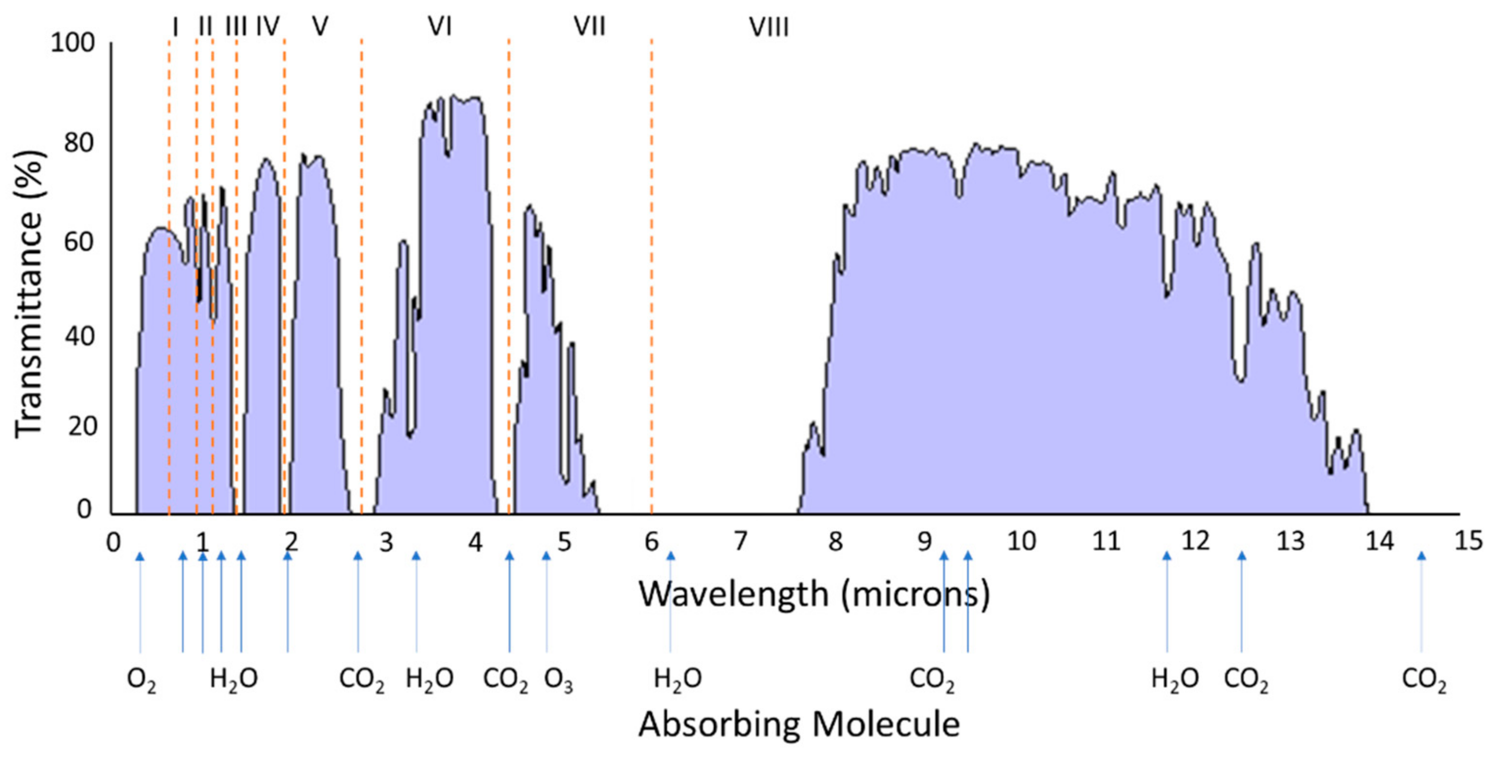
| Window Number | Window Boundaries (µm) |
|---|---|
| I | 0.72–0.94 |
| II | 0.94–1.13 |
| III | 1.13–1.38 |
| IV | 1.38–1.90 |
| V | 1.90–2.70 |
| VI | 2.70–4.30 |
| VII | 4.30–6.00 |
| Type of Scattering | Size of Scatterer |
|---|---|
| Rayleigh Scattering | Electron Size of Scatterer |
| Mie Scattering | Size of Scatterer ≈ |
| Non-selective Scattering | Size of Scatterer |
| Source | Amount, Tg/yr [106 Metric Tons/yr] | |
|---|---|---|
| Range | Best Estimate | |
| Natural | ||
| Soil Dust | 1000–3000 | 1500 |
| Sea Salt | 1000–10,000 | 1300 |
| Botanical Debris | 26–80 | 50 |
| Volcanic Dust | 4–10,000 | 30 |
| Forest Fires | 3–1500 | 20 |
| Gas-to-particle conversion (total) | 100–260 | 180 |
| Sulphate from H2S | 130–200 | |
| Ammonium salts from NH3 | 80–270 | |
| Nitrate from NOx | 60–430 | |
| Hydrocarbons from plant exudations | 75–200 | |
| Photochemical | 40–200 | 60 |
| Subtotal | 2200–24,000 | 3100 |
| Anthropogenic | ||
| Direct Emissions | 50–160 | 120 |
| Gas-to-particle conversion (total) | 260–460 | 330 |
| Sulphate from SO2 | 130–200 | |
| Nitrate from NOx | 30–35 | |
| Hydrocarbons | 15–90 | |
| Photochemical | 5–25 | 10 |
| Subtotal | 320–640 | 460 |
| Rainfall Rate (cm/h) | Transmittance, τ, for 1800 m Path |
|---|---|
| 0.25 | 0.88 |
| 1.25 | 0.74 |
| 2.5 | 0.65 |
| 10.0 | 0.38 |
| Rain Intensity | Rainfall (mm/h) |
|---|---|
| Mist | 0.025 |
| Drizzle | 0.25 |
| Light | 1.0 |
| Moderate | 4.0 |
| Heavy | 16 |
| Thundershower | 40 |
| Cloudburst | 100 |
| Turbulence Strength | Refractive Index Structure Coefficient, |
|---|---|
| Strong | [m−2/3] |
| Intermediate | [m−2/3] |
| Weak | [m−2/3] |
| Reference | ||||
|---|---|---|---|---|
| Fried’s Model | 1/3 | 3200 m | [70] | |
| Brookner’s Model | 5/6 | 320 m | [71] | |
| Tatarski’s Model | 4/3 | ∞ | [72] | |
| Hufnagel Condition I | −10 | 1000 m | [73] | |
| Hufnagel Condition II | 0 | 1500 m | [73] |
| Equation | Ref. | ||
|---|---|---|---|
| Fried’s Model | (22) | [70] | |
| Brookner’s Model | (23) | [71] | |
| Tatarski’s Model | (24) | [72] | |
| Hufnagel Model | (25) | [73] |
| Altitude (km) | |
|---|---|
| 0.001 | 30 |
| 0.003 | 20 |
| 0.01 | 15 |
| 0.03 | 10 |
| 0.1 | 6 |
| 0.3 | 4 |
| 1.0 | 1 |
| 3.0 | 1 |
| Constants | ||||
|---|---|---|---|---|
| Window | ||||
| I | 0.0305 | 0.800 | 0.112 | 54 |
| II | 0.0363 | 0.765 | 0.134 | 54 |
| III | 0.1303 | 0.830 | 0.093 | 2.0 |
| IV | 0.211 | 0.802 | 0.111 | 1.1 |
| V | 0.350 | 0.814 | 0.1035 | 0.35 |
| VI | 0.373 | 0.827 | 0.095 | 0.26 |
| VII | 0.598 | 0.784 | 0.122 | 0.165 |
| Case | Condition | Equations | |
|---|---|---|---|
| A | (69) | ||
| B | (70) | ||
| C | (71) | ||
| D | (72) | ||
| R1 | Rain | (73) | |
| R2 | Rain | (74) |
| Areas of Contribution | ML Algorithms | References | |
|---|---|---|---|
| Algorithms | Their Functions | ||
| SNR improvement | GPML | Filtering | [105] |
| SVM, random forest, decision tree, gradient boosting tree | Supervised learning | [106] | |
| CNN | Supervised learning | [107] | |
| Smoke detection | t-SNE, density-based spatial clustering | Clustering | [106] |
| Cirrus cloud detection | CNN | Supervised learning | [107] |
| Improving the prediction accuracy | RNN, CNN, RNN-CNN | Supervised learning in sensor fusion | [108] |
| Dealing with atmospheric turbulence | ANN | Supervised learning | [109] |
Publisher’s Note: MDPI stays neutral with regard to jurisdictional claims in published maps and institutional affiliations. |
© 2021 by the authors. Licensee MDPI, Basel, Switzerland. This article is an open access article distributed under the terms and conditions of the Creative Commons Attribution (CC BY) license (https://creativecommons.org/licenses/by/4.0/).
Share and Cite
Fahey, T.; Islam, M.; Gardi, A.; Sabatini, R. Laser Beam Atmospheric Propagation Modelling for Aerospace LIDAR Applications. Atmosphere 2021, 12, 918. https://doi.org/10.3390/atmos12070918
Fahey T, Islam M, Gardi A, Sabatini R. Laser Beam Atmospheric Propagation Modelling for Aerospace LIDAR Applications. Atmosphere. 2021; 12(7):918. https://doi.org/10.3390/atmos12070918
Chicago/Turabian StyleFahey, Thomas, Maidul Islam, Alessandro Gardi, and Roberto Sabatini. 2021. "Laser Beam Atmospheric Propagation Modelling for Aerospace LIDAR Applications" Atmosphere 12, no. 7: 918. https://doi.org/10.3390/atmos12070918