
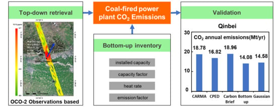
Estimating CO2 Emissions from Large Scale Coal-Fired Power Plants Using OCO-2 Observations and Emission Inventories

Abstract
:
1. Introduction
2. Materials and Methods
2.1. Data
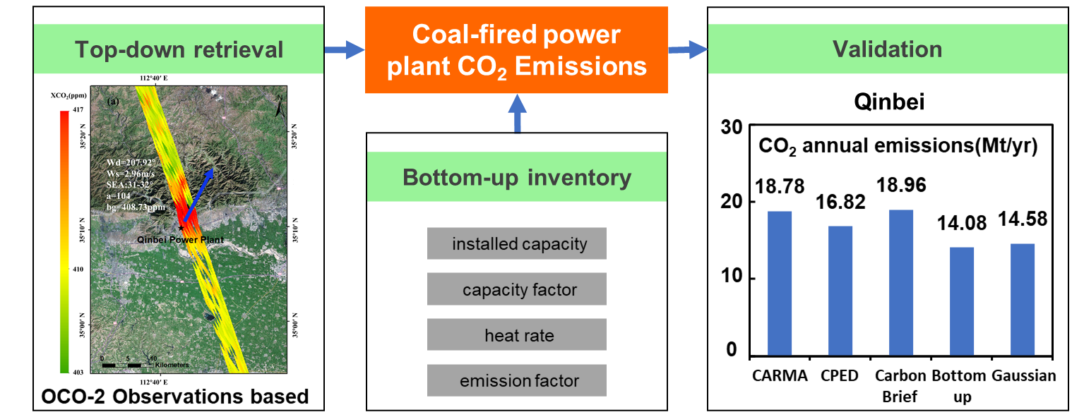
2.1.1. Power Plant Data
2.1.2. Orbiting Carbon Observatory-2 (OCO-2) Data
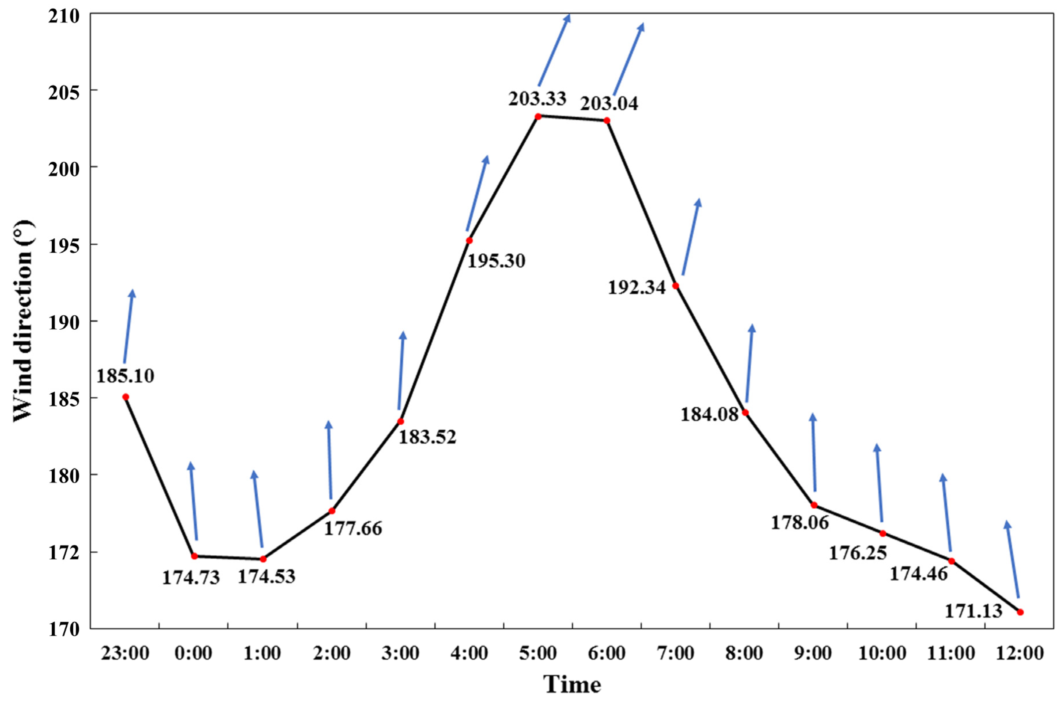
2.1.3. Wind Data
2.2. Gaussian Plume Model
2.3. Bottom-Up Estimates
3. Results
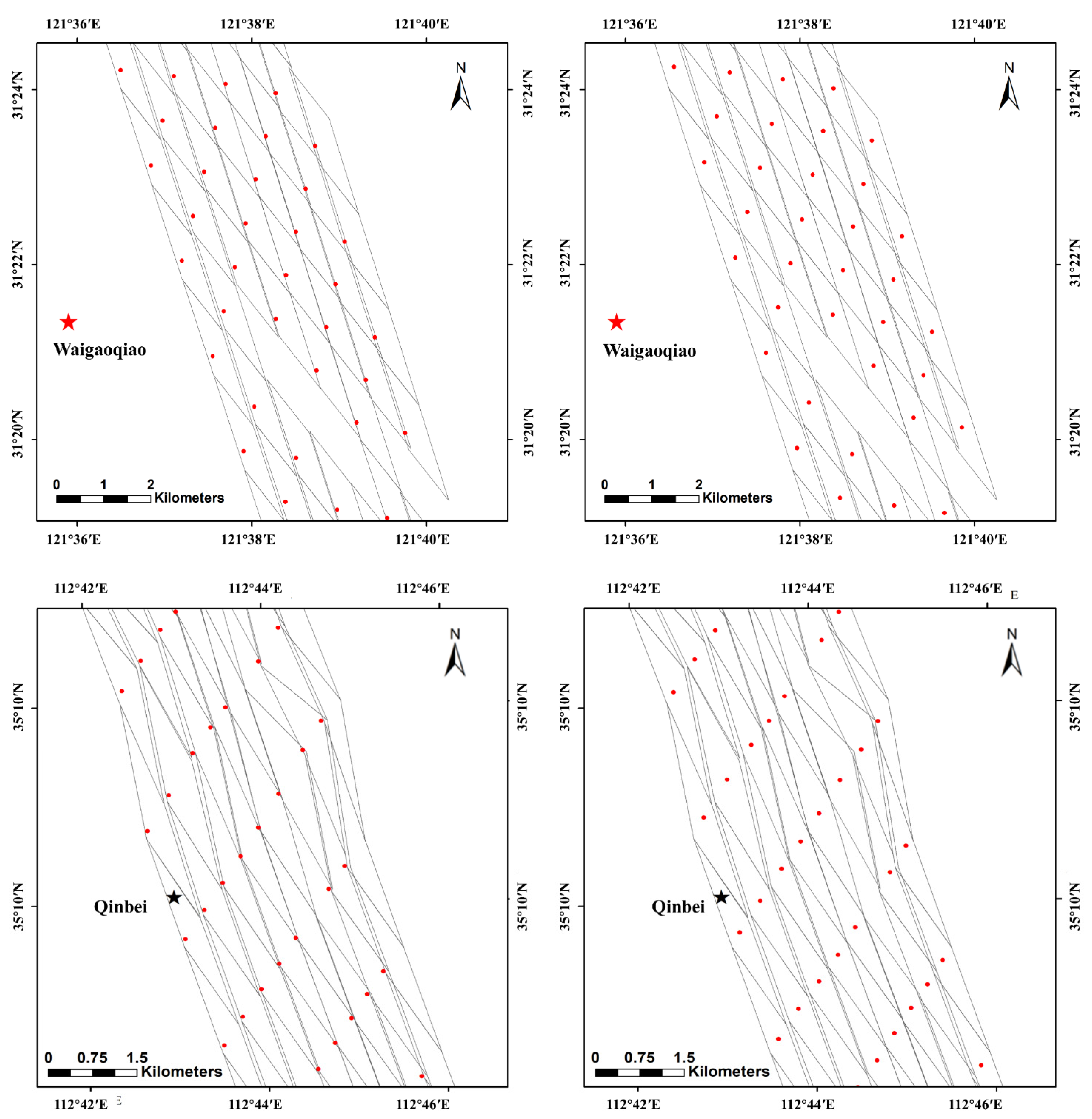
3.1. Screening
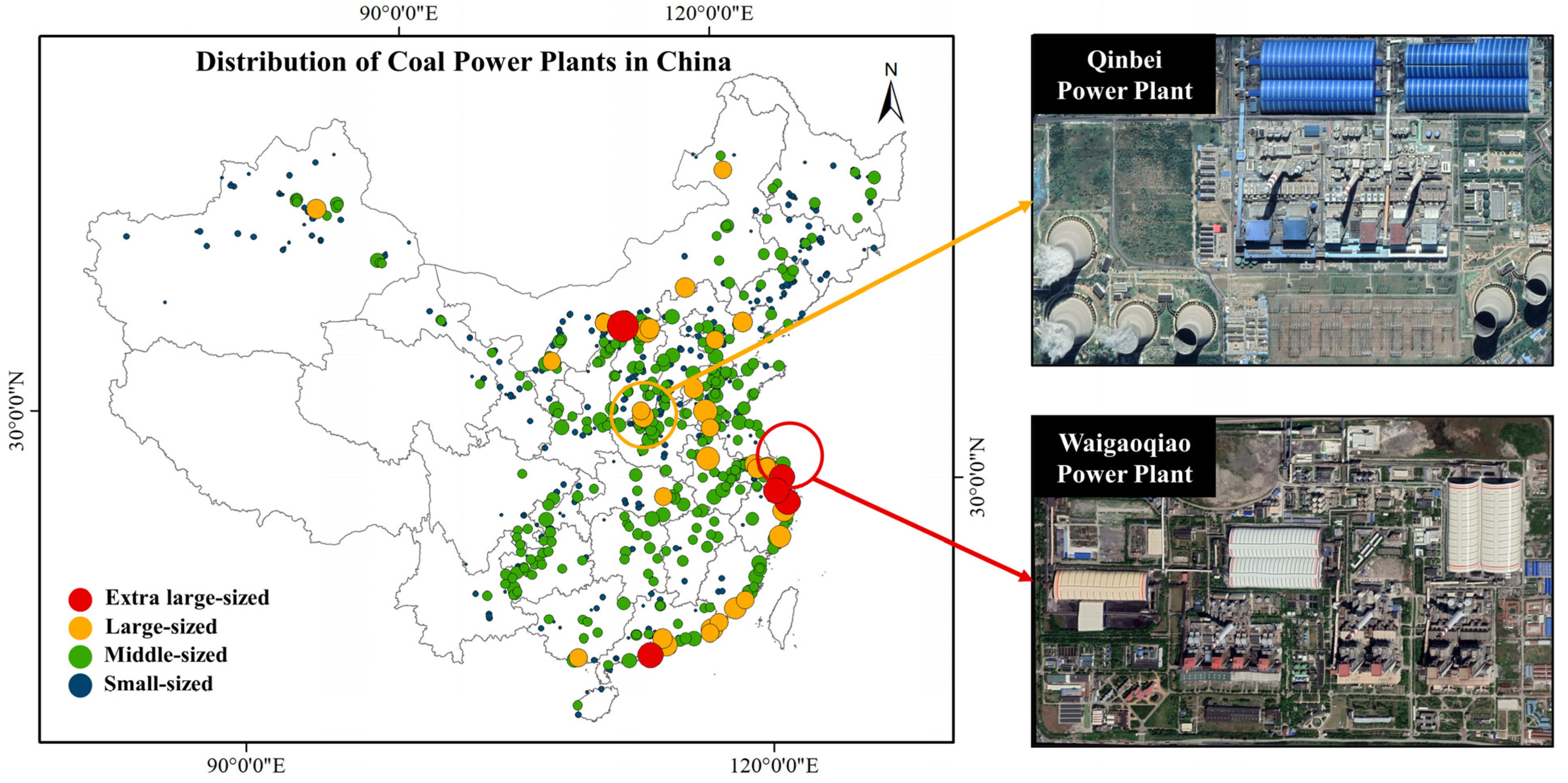
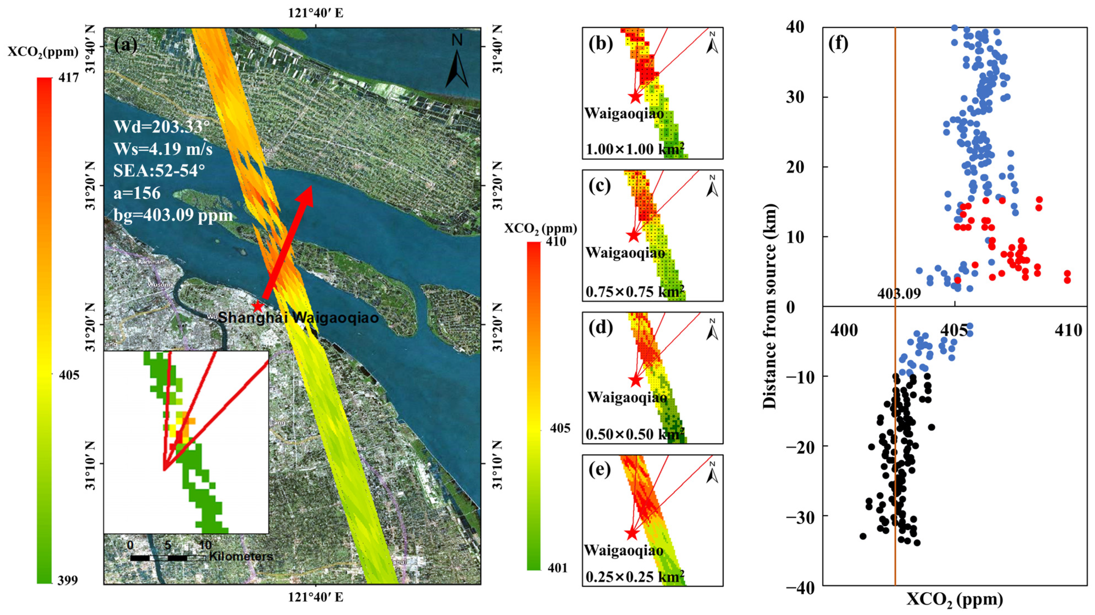
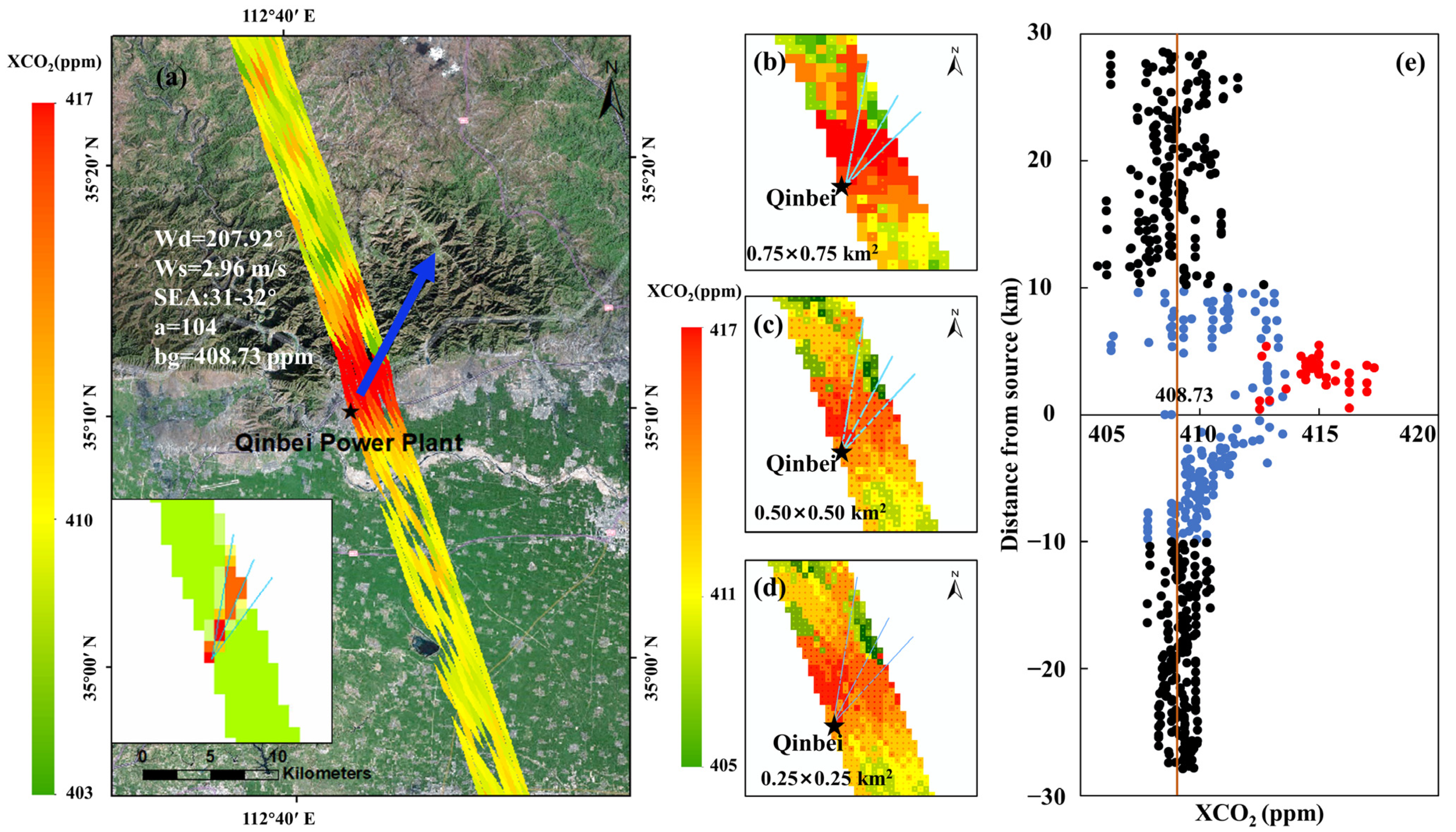
3.2. Configuration
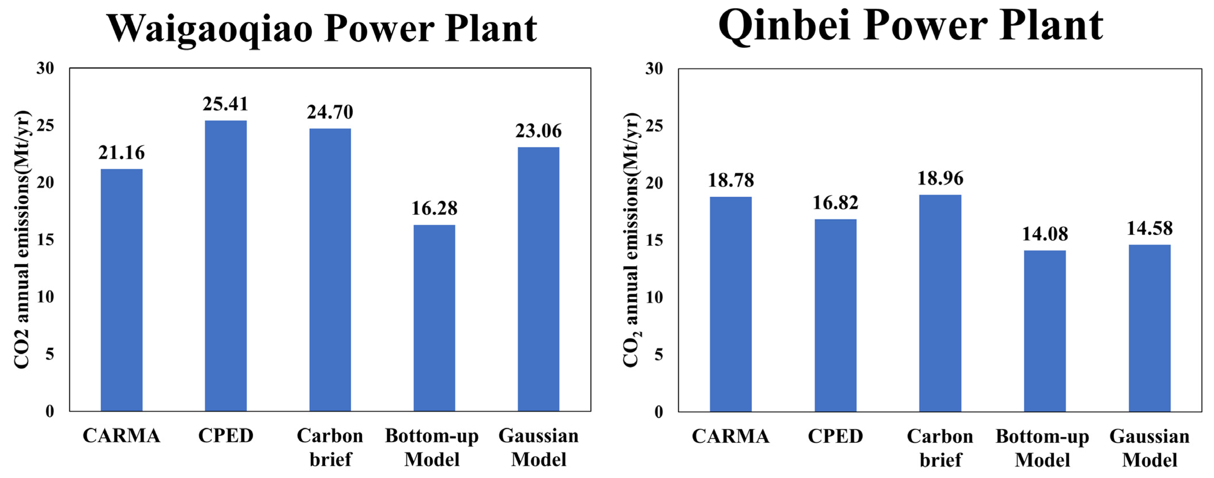
3.3. Estimated Emissions
3.4. Bottom-Up Estimations
4. Discussion
4.1. Power Plant Screening
4.2. Estimation Details and Validation of Emissions
4.3. Limitation and Prospects
5. Conclusions
Author Contributions
Funding
Data Availability Statement
Acknowledgments
Conflicts of Interest
References
- Oda, T.; Maksyutov, S.; Andres, R.J. The Open-source Data Inventory for Anthropogenic CO2, version 2016 (ODIAC2016): A global monthly fossil fuel CO2 gridded emissions data product for tracer transport simulations and surface flux inversions. Earth Syst. Sci. Data 2018, 10, 87–107. [Google Scholar] [CrossRef] [Green Version]
- The Intergovernmental Panel on Climate Change. Climate Change 2014: Synthesis Report, Contribution of Working Groups I, II and III to the Fifth Assessment Report of the Intergovernmental Panel on Climate Change; Core Writing Team, Pachauri, R.K., Meyer, L.A., Eds.; IPCC: Geneva, Switzerland, 2014. [Google Scholar]
- Reuter, M.; Buchwitz, M.; Schneising, O.; Krautwurst, S.; O’Dell, C.W.; Richter, A.; Bovensmann, H.; Burrows, J.P. Towards monitoring localized CO2 emissions from space: Co-located regional CO2 and NO2 enhancements observed by the OCO-2 and S5P satellites. Atmos. Chem. Phys. 2019, 19, 9371–9383. [Google Scholar] [CrossRef] [Green Version]
- Rockström, J.; Gaffney, O.; Rogelj, J.; Meinshausen, M.; Nakicenovic, N.; Schellnhuber, H.J. A roadmap for rapid decarbonization. Science 2017, 355, 1269. [Google Scholar] [CrossRef] [PubMed] [Green Version]
- Crippa, M.; Oreggioni, G.; Guizzardi, D.; Muntean, M.; Schaaf, E.; Lo Vullo, E.; Solazzo, E.; Monforti-Ferrario, F.; Olivier, J.G.J.; Vignati, E. Fossil CO2 and GHG Emissions of All World Countries—2019 Report; Publications Office of the European Union: Luxembourg, 2019. [Google Scholar]
- Crippa, M.; Guizzardi, D.; Muntean, M.; Schaaf, E.; Lo Vullo, E.; Solazzo, E.; Monforti-Ferrario, F.; Olivier, J.; Vignati, E. EDGAR v5.0 Greenhouse Gas Emissions; European Commission, Joint Research Center (JRC): Brussels, Belgium, 2019; Available online: http://data.europa.eu/89h/488dc3de-f072-4810-ab83-47185158ce2a (accessed on 22 November 2020).
- Zheng, B.; Tong, D.; Li, M.; Liu, F.; Hong, C.; Geng, G.; Li, H.; Li, X.; Peng, L.; Qi, J.; et al. Trends in China’s anthropogenic emissions since 2010 as the consequence of clean air actions. Atmos. Chem. Phys. 2018, 18, 14095–14111. [Google Scholar] [CrossRef] [Green Version]
- Decola, P.; Tarasova, O. An Integrated Global Greenhouse Gas Information System (IG3IS). Available online: https://public.wmo.int/en/resources/bulletin/integrated-global-greenhouse-gas-information-system-ig3is (accessed on 30 November 2020).
- Ciais, P.; Dolman, A.J.; Bombelli, A.; Duren, R.; Peregon, A.; Rayner, P.J.; Miller, C.; Gobron, N.; Kinderman, G.; Marland, G.; et al. Current systematic carbon-cycle observations and the need for implementing a policy-relevant carbon observing system. Biogeosciences 2014, 11, 3547–3602. [Google Scholar] [CrossRef] [Green Version]
- Boden, T.A.; Marland, G.; Andres, R.J. Global, Regional, and National Fossil-Fuel CO2 Emissions (1751–2014); Carbon Dioxide Information Analysis Center (CDIAC), Oak Ridge National Laboratory (ORNL): Oak Ridge, TN, USA, 2017. [Google Scholar] [CrossRef]
- Le Quéré, C.; Andrew, R.M.; Canadell, J.G.; Sitch, S.; Korsbakken, J.I.; Peters, G.P.; Manning, A.C.; Boden, T.A.; Tans, P.P.; Houghton, R.A.; et al. Global Carbon Budget 2016. Earth Syst. Sci. Data 2016, 8, 605–649. [Google Scholar] [CrossRef] [Green Version]
- Kuze, A.; Suto, H.; Shiomi, K.; Kawakami, S.; Tanaka, M.; Ueda, Y.; Deguchi, A.; Yoshida, J.; Yamamoto, Y.; Kataoka, F.; et al. Update on GOSAT TANSO-FTS performance, operations, and data products after more than 6 years in space. Atmos. Meas. Tech. 2016, 9, 2445–2461. [Google Scholar] [CrossRef] [Green Version]
- Crisp, D.; Pollock, H.R.; Rosenberg, R.; Chapsky, L.; Lee, R.A.M.; Oyafuso, F.A.; Frankenberg, C.; O’Dell, C.W.; Bruegge, C.J.; Doran, G.B.; et al. The on-orbit performance of the Orbiting Carbon Observatory-2 (OCO-2) instrument and its radiometrically calibrated products. Atmos. Meas. Tech. 2017, 10, 59–81. [Google Scholar] [CrossRef] [Green Version]
- Wunch, D.; Wennberg, P.O.; Osterman, G.; Fisher, B.; Naylor, B.; Roehl, C.M.; O’Dell, C.; Mandrake, L.; Viatte, C.; Kiel, M.; et al. Comparisons of the Orbiting Carbon Observatory-2 (OCO-2) XCO2 measurements with TCCON. Atmos. Meas. Tech. 2017, 10, 2209–2238. [Google Scholar] [CrossRef] [Green Version]
- Hakkarainen, J.; Ialongo, I.; Tamminen, J. Direct space-based observations of anthropogenic CO2 emission areas from OCO-2. Geophys. Res. Lett. 2016, 43, 11400–11406. [Google Scholar] [CrossRef]
- Janardanan, R.; Maksyutov, S.; Oda, T.; Saito, M.; Kaiser, J.W.; Ganshin, A.; Stohl, A.; Matsunaga, T.; Yoshida, Y.; Yokota, T. Comparing GOSAT observations of localized CO2 enhancements by large emitters with inventory-based estimates. Geophys. Res. Lett. 2016, 43, 3486–3493. [Google Scholar] [CrossRef] [Green Version]
- Lauvaux, T.; Miles, N.L.; Deng, A.; Richardson, S.J.; Cambaliza, M.O.; Davis, K.J.; Gaudet, B.; Gurney, K.R.; Huang, J.; O’Keefe, D.; et al. High-resolution atmospheric inversion of urban CO2 emissions during the dormant season of the Indianapolis Flux Experiment (INFLUX). J. Geophys. Res. Atmos. 2016, 121, 5213–5236. [Google Scholar] [CrossRef] [Green Version]
- Nickless, A.; Rayner, P.J.; Engelbrecht, F.; Brunke, E.G.; Erni, B.; Scholes, R.J. Estimates of CO2 fluxes over the city of Cape Town, South Africa, through Bayesian inverse modelling. Atmos. Chem. Phys. 2018, 18, 4765–4801. [Google Scholar] [CrossRef] [Green Version]
- Sargent, M.; Barrera, Y.; Nehrkorn, T.; Hutyra, L.R.; Gately, C.K.; Jones, T.; McKain, K.; Sweeney, C.; Hegarty, J.; Hardiman, B.; et al. Anthropogenic and biogenic CO2 fluxes in the Boston urban region. Proc. Natl. Acad. Sci. USA 2018, 115, 7491–7496. [Google Scholar] [CrossRef] [Green Version]
- Bovensmann, H.; Buchwitz, M.; Burrows, J.P.; Reuter, M.; Krings, T.; Gerilowski, K.; Schneising, O.; Heymann, J.; Tretner, A.; Erzinger, J. A remote sensing technique for global monitoring of power plant CO2 emissions from space and related applications. Atmos. Meas. Tech. 2010, 3, 781–811. [Google Scholar] [CrossRef] [Green Version]
- Nassar, R.; Hill, T.G.; McLinden, C.A.; Wunch, D.; Jones, D.B.A.; Crisp, D. Quantifying CO2 Emissions from Individual Power Plants from Space. Geophys. Res. Lett. 2017, 44, 10045–10053. [Google Scholar] [CrossRef] [Green Version]
- Krings, T.; Neininger, B.; Gerilowski, K.; Krautwurst, S.; Buchwitz, M.; Burrows, J.P.; Lindemann, C.; Ruhtz, T.; Schüttemeyer, D.; Bovensmann, H. Airborne remote sensing and in situ measurements of atmospheric CO2 to quantify point source emissions. Atmos. Meas. Tech. 2018, 11, 721–739. [Google Scholar] [CrossRef] [Green Version]
- Zheng, T.; Nassar, R.; Baxter, M. Estimating power plant CO2 emission using OCO-2 XCO2 and high resolution WRF-Chem simulations. Environ. Res. Lett. 2019, 14, 085001. [Google Scholar] [CrossRef]
- Randy, P.; Robert, E.H.; James, R.H.; Dean, L.J.; Andrea, K.; David, M.; Charles, P.; David, R.; David, R.; Jose, R.; et al. The Orbiting Carbon Observatory instrument: Performance of the OCO instrument and plans for the OCO-2 instrument. In Proceedings of the Sensors, Systems, and Next-Generation Satellites XIV, Proc. SPIE 7826, Toulouse, France, 13 October 2010. [Google Scholar] [CrossRef]
- Hersbach, H.; Bell, B.; Berrisford, P.; Biavati, G.; Horányi, A.; Muñoz Sabater, J.; Nicolas, J.; Peubey, C.; Radu, R.; Rozum, I.; et al. ERA5 Hourly Data on Pressure Levels from 1979 to Present. Copernicus Climate Change Service (C3S) Climate Data Store (CDS). 2018. Available online: https://cds.climate.copernicus.eu/cdsapp#!/dataset/reanalysis-era5-pressure-levels?tab=overview (accessed on 23 June 2021).
- Global Modeling and Assimilation Office (GMAO). MERRA-2 tavg3_3d_asm_Nv: 3d,3-Hourly, Time-Averaged, Model-Level, Assimilation, Assimilated Meteorological Fields; Goddard Earth Sciences Data and Information Services Center (GES DISC): Greenbelt, MD, USA, 2015. [Google Scholar] [CrossRef]
- Molod, A.; Takacs, L.; Suarez, M.; Bacmeister, J. Development of the GEOS-5 atmospheric general circulation model: Evolution from MERRA to MERRA2. Geosci. Model Dev. 2015, 8, 1339–1356. [Google Scholar] [CrossRef] [Green Version]
- Hersbach, H.; Bell, B.; Berrisford, P.; Hirahara, S.; Horányi, A.; Muñoz-Sabater, J.; Nicolas, J.; Peubey, C.; Radu, R.; Schepers, D.; et al. The ERA5 global reanalysis. Q. J. R. Meteorol. Soc. 2020, 146, 1999–2049. [Google Scholar] [CrossRef]
- Arystanbekova, N.K. Application of Gaussian plume models for air pollution simulation at instantaneous emissions. Math. Comput. Simul. 2004, 67, 451–458. [Google Scholar] [CrossRef]
- Pasquill, F. The Estimation of Dispersion of Windborne Material. Meteorol. Mag. 1961, 90, 33–40. [Google Scholar]
- Martin, D.O. Comment On “The Change of Concentration Standard Deviations with Distance”. J. Air Pollut. Control Assoc. 1976, 26, 145–147. [Google Scholar] [CrossRef] [Green Version]
- Shim, C.; Han, J.; Henze, D.K.; Yoon, T. Identifying local anthropogenic CO2 emissions with satellite retrievals: A case study in South Korea. Int. J. Remote Sens. 2018, 40, 1011–1029. [Google Scholar] [CrossRef] [Green Version]
- Gordon, M.; Li, S.M.; Staebler, R.; Darlington, A.; Hayden, K.; O’Brien, J.; Wolde, M. Determining air pollutant emission rates based on mass balance using airborne measurement data over the Alberta oil sands operations. Atmos. Meas. Tech. 2015, 8, 3745–3765. [Google Scholar] [CrossRef] [Green Version]
- Ummel, K. CARMA Revisited: An Updated Database of Carbon Dioxide Emissions from Power Plants Worldwide; Working Paper 304; Center for Global Development: Washington, DC, USA, 2012; Available online: http://www.cgdev.org/content/publications/detail/1426429 (accessed on 2 November 2020).
- Wheeler, D.; Ummel, K.C. Calculating CARMA: Global Estimation of CO2 Emissions from the Power Sector; Working Paper 145; Center for Global Development: Washington, DC, USA, 2008. [Google Scholar]
- Liu, F.; Zhang, Q.; Tong, D.; Zheng, B.; Li, M.; Huo, H.; He, K.B. High-resolution inventory of technologies, activities, and emissions of coal-fired power plants in China from 1990 to 2010. Atmos. Chem. Phys. 2015, 15, 13299–13317. [Google Scholar] [CrossRef] [Green Version]
- Global Energy Monitor Contributors. Estimating Carbon Dioxide Emissions from Coal Plants. Available online: https://www.gem.wiki/w/index.php?title=Estimating_carbon_dioxide_emissions_from_coal_plants&oldid=215845 (accessed on 24 November 2020).
- Sargent & Lundy, L.L.C. New Coal-Fired Power Plant. Performance and Cost Estimates; The U.S. Environmental Protection Agency: Chicago, IL, USA, 2009. Available online: https://www.epa.gov/airmarkets/new-coal-fired-power-plant-performance-and-cost-estimates (accessed on 2 September 2020).
- Beér, J.M. High efficiency electric power generation: The environmental role. Prog. Energy Combust. Sci. 2007, 33, 107–134. [Google Scholar] [CrossRef] [Green Version]
- The Intergovernmental Panel on Climate Change. 2006 IPCC Guidelines for National Greenhouse Gas. Inventories; Eggleston, H.S.B.L., Miwa, K., Ngara, T., Tanabe, K., Eds.; IPCC National Greenhouse Gas Inventories Programme, Intergovernmental Panel on Climate Change IPCC; c/o Institute for Global Environmental Strategies IGES: Kanagawa, Japan, 2006. [Google Scholar]
- Kiel, M.; O’Dell, C.W.; Fisher, B.; Eldering, A.; Nassar, R.; MacDonald, C.G.; Wennberg, P.O. How bias correction goes wrong: Measurement of XCO2 affected by erroneous surface pressure estimates. Atmos. Meas. Tech. 2019, 12, 2241–2259. [Google Scholar] [CrossRef] [Green Version]
- Zheng, B.; Chevallier, F.; Ciais, P.; Broquet, G.; Wang, Y.; Lian, J.; Zhao, Y. Observing carbon dioxide emissions over China’s cities and industrial areas with the Orbiting Carbon Observatory-2. Atmos. Chem. Phys. 2020, 20, 8501–8510. [Google Scholar] [CrossRef]
- Stubenrauch, C.J.; Rossow, W.B.; Kinne, S.; Ackerman, S.; Cesana, G.; Chepfer, H.; Di Girolamo, L.; Getzewich, B.; Guignard, A.; Heidinger, A.; et al. Assessment of Global Cloud Datasets from Satellites: Project and Database Initiated by the GEWEX Radiation Panel. Bull. Am. Meteorol. Soc. 2013, 94, 1031–1049. [Google Scholar] [CrossRef]
- Shakeb, A.; Eric, N. Carbon Monitoring for Action (CARMA): Climate Campaign Built on Questionable Data—A due Diligence Report on CARMA’s Data and Methodology. 2008. Available online: http://dx.doi.org/10.2139/ssrn.1133432 (accessed on 2 September 2020).
- Wang, Y.; Broquet, G.; Bréon, F.M.; Lespinas, F.; Buchwitz, M.; Reuter, M.; Meijer, Y.; Loescher, A.; Janssens-Maenhout, G.; Zheng, B.; et al. PMIF v1.0: Assessing the potential of satellite observations to constrain CO2 emissions from large cities and point sources over the globe using synthetic data. Geosci. Model Dev. 2020, 13, 5813–5831. [Google Scholar] [CrossRef]
- Kort, E.A.; Frankenberg, C.; Miller, C.E.; Oda, T. Space-based observations of megacity carbon dioxide. Geophys. Res. Lett. 2012, 39, L17806. [Google Scholar] [CrossRef] [Green Version]
- Cai, Z.; Liu, Y.; Yang, D. Analysis of XCO2 retrieval sensitivity using simulated Chinese Carbon Satellite (TanSat) measurements. Sci. China Earth Sci. 2014, 57, 1919–1928. [Google Scholar] [CrossRef]
- Taylor, T.E.; Eldering, A.; Merrelli, A.; Kiel, M.; Somkuti, P.; Cheng, C.; Rosenberg, R.; Fisher, B.; Crisp, D.; Basilio, R.; et al. OCO-3 early mission operations and initial (vEarly) XCO2 and SIF retrievals. Remote Sens. Environ. 2020, 251, 112032. [Google Scholar] [CrossRef]
- OCO Science Team; Gunson, M.; Eldering, A. OCO-3 Level 2 Bias-Corrected XCO2 and Other Select Fields from the Full-Physics Retrieval Aggregated as Daily Files, Retrospective Processing VEarlyR; Goddard Earth Sciences Data and Information Services Center (GES DISC): Greenbelt, MD, USA, 2020. Available online: https://disc.gsfc.nasa.gov/datacollection/OCO3_L2_Lite_FP_EarlyR.html (accessed on 2 September 2020).
- Kuhlmann, G.; Broquet, G.; Marshall, J.; Clément, V.; Löscher, A.; Meijer, Y.; Brunner, D. Detectability of CO2 emission plumes of cities and power plants with the Copernicus Anthropogenic CO2 Monitoring (CO2M) mission. Atmos. Meas. Tech. 2019, 12, 6695–6719. [Google Scholar] [CrossRef] [Green Version]
- Hill, T.; Nassar, R. Pixel Size and Revisit Rate Requirements for Monitoring Power Plant CO2 Emissions from Space. Remote Sens. 2019, 11, 1608. [Google Scholar] [CrossRef] [Green Version]


| Coal Power Plant | Province | Capacity (MW) | Date | OCO-2 Mode | Overpass Hour in UTC | Configuration | Number of OCO-2 Points in Plume |
|---|---|---|---|---|---|---|---|
| Waigaoqiao | Shanghai | 5000 | 12 March 2015 | Glint | 5:01 | Flyby (~2.3 km) | 29 |
| Qinbei | Henan | 4400 | 24 November 2017 | Glint | 5:27 | Overpass | 6 |
| Power Plant | Resolution | Number of OCO-2 Points in Plume | R | Annual CO2 Emissions (Mt/yr) |
|---|---|---|---|---|
| Waigaoqiao | 1.00 × 1.00 km2 | 31 | R1 = 0.75 | 22.57 |
| 0.75 × 0.75 km2 | 75 | R2 = 0.83 | 23.09 | |
| 0.50 × 0.50 km2 | 102 | R3 = 0.90 | 23.06 | |
| 0.25 × 0.25 km2 | 438 | R4 = 0.86 | 21.99 | |
| Qinbei | 0.75 × 0.75 km2 | 19 | – | – |
| 0.50 × 0.50 km2 | 41 | R2 = 0.71 | 14.86 | |
| 0.25 × 0.25 km2 | 80 | R3 = 0.79 | 14.58 |
| Power Plant | Units | Capacity (MW) | Power Generation (TWh) | Capacity Factor (%) | Heat Rate (Btu/kWh) | Emission Factor (kg/TJ) | CO2 Emissions (Mt/yr) |
|---|---|---|---|---|---|---|---|
| Waigaoqiao | 1–4 | 300 | 3.12 | 29.70 | 8863 | 94,600 | 16.28 |
| 5–6 | 900 | 7.82 | 49.61 | 8540 | |||
| 7–8 | 1000 | 9.59 | 54.72 | 7896 | |||
| Qinbei | 1–2 | 600 | 16.60 | 43.07 | 8564 | 94,600 | 14.08 |
| 3–4 | 600 | 8564 | |||||
| 5–6 | 1000 | 8418 |
| Power Plant | Date | Background | N | Report (kt/d) | N17 (kt/d) | RN | Estimation (kt/d) | R |
|---|---|---|---|---|---|---|---|---|
| Westar | 4 December 2015 | 400.96 ppm | 130 | 26.67 | 31.21 | 0.468 | 24.95 | 0.751 |
| Ghent | 13 August 2015 | 392.67 ppm | 33 | 29.17 | 29.46 | 0.707 | 28.94 | 0.824 |
| Gavin/Kyger | 30 July 2015 | 396.62 ppm | 17 | 50.54 | 48.66 | 0.688 | 51.03 | 0.812 |
| Power Plant | Total Uncertainty (Mt/year) | Wind Speed Uncertainty (Mt/year) | Background Uncertainty (Mt/year) | Enhance Uncertainty (Mt/year) | Secondary Uncertainty (Mt/year) | Interpolation Uncertainty (Mt/year) |
|---|---|---|---|---|---|---|
| Waigaoqiao | 2.86 | 2.59 | 0.22 | 1.10 | – | 0.45 |
| Qinbei | 3.38 | 3.12 | 0.30 | 1.25 | – | 0.14 |
Publisher’s Note: MDPI stays neutral with regard to jurisdictional claims in published maps and institutional affiliations. |
© 2021 by the authors. Licensee MDPI, Basel, Switzerland. This article is an open access article distributed under the terms and conditions of the Creative Commons Attribution (CC BY) license (https://creativecommons.org/licenses/by/4.0/).
Share and Cite
Hu, Y.; Shi, Y. Estimating CO2 Emissions from Large Scale Coal-Fired Power Plants Using OCO-2 Observations and Emission Inventories. Atmosphere 2021, 12, 811. https://doi.org/10.3390/atmos12070811
Hu Y, Shi Y. Estimating CO2 Emissions from Large Scale Coal-Fired Power Plants Using OCO-2 Observations and Emission Inventories. Atmosphere. 2021; 12(7):811. https://doi.org/10.3390/atmos12070811
Chicago/Turabian StyleHu, Yaqin, and Yusheng Shi. 2021. "Estimating CO2 Emissions from Large Scale Coal-Fired Power Plants Using OCO-2 Observations and Emission Inventories" Atmosphere 12, no. 7: 811. https://doi.org/10.3390/atmos12070811