Data Intelligence Model and Meta-Heuristic Algorithms-Based Pan Evaporation Modelling in Two Different Agro-Climatic Zones: A Case Study from Northern India

Abstract

Precise quantification of evaporation has a vital role in effective crop modelling, irrigation scheduling, and agricultural water management. In recent years, the data-driven models using meta-heuristics algorithms have attracted the attention of researchers worldwide. In this investigation, we have examined the performance of models employing four meta-heuristic algorithms, namely, support vector machine (SVM), random tree (RT), reduced error pruning tree (REPTree), and random subspace (RSS) for simulating daily pan evaporation (EP_d) at two different locations in north India representing semi-arid climate (New Delhi) and sub-humid climate (Ludhiana). The most suitable combinations of meteorological input variables as covariates to estimate EP_d were ascertained through the subset regression technique followed by sensitivity analyses. The statistical indicators such as root mean square error (RMSE), mean absolute error (MAE), Nash–Sutcliffe efficiency (NSE), Willmott index (WI), and correlation coefficient (r) followed by graphical interpretations, were utilized for model evaluation. The SVM algorithm successfully performed in reconstructing the EP_d time series with acceptable statistical criteria (i.e., NSE = 0.937, 0.795; WI = 0.984, 0.943; r = 0.968, 0.902; MAE = 0.055, 0.993 mm/day; and RMSE = 0.092, 1.317 mm/day) compared with the other applied algorithms during the testing phase at the New Delhi and Ludhiana stations, respectively. This study also demonstrated and discussed the potential of meta-heuristic algorithms for producing reasonable estimates of daily evaporation using minimal meteorological input variables with applicability of the best candidate model vetted in two diverse agro-climatic settings.

1. Introduction

The hydrological process by which the liquid water from water bodies and landmass is converted to vapor and transferred to the atmosphere is known as evaporation, which is a significant constituent member of the hydrological cycle. The driving factor for this process is the pressure gradient between the atmosphere–earth system [1,2]. Water scarcity has become a serious concern and evaporation losses have increased significantly during the last few decades; therefore, precise estimation of evaporation is crucial, particularly in regions of limited water resources [3,4,5]. Evaporation losses alone account for 61% of the global precipitation. Daily pan evaporation (EP_d) has been extensively used in irrigation scheduling, water balance studies, sustainable water resources management, and hydrological modelling, etc. [2,6,7,8].

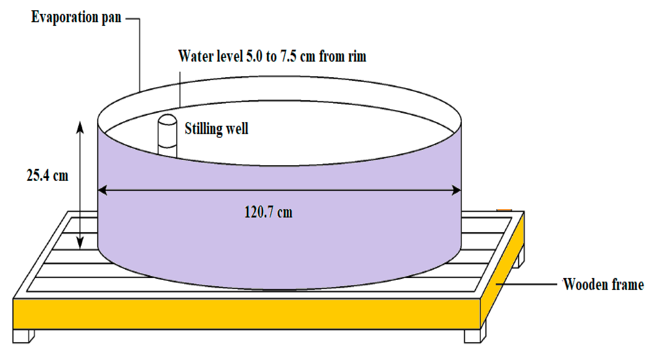
In most cases, evaporation is quantified using the direct approach (i.e., pan evaporimeter) [9]. Pan-evaporimeter-based evaporation losses measurement is an ancient and widely used technique [1,10,11]. The class A type pan, developed in the United States by the National Weather Service (NWS), has standardized dimensions having a diameter of 120.7 cm, depth of 25.4 cm, and placed at 15 cm above the ground surface [1,12]. Although pan evaporation gives realistic measurements, it has limitations in high initial and maintenance costs [10,11]. In the absence of direct measurement, complexities arising from near-surface climatic conditions pose difficulties in developing universal and explicit expressions to compute evaporation [2,13,14]. Most of the meteorological variables, such as temperature (maximum and minimum), wind speed (WS), relative humidity (RH), vapor pressure and others have a substantial role in influencing the processes leading to evaporation [1,15]. Therefore, these variables in their individual capacities or in combinations contributed to various models and approaches to estimate evaporation in areas where direct measurements were not done.

In the advent of soft computing tools, developments in data-driven models using meta-heuristic algorithms have been incorporated to model various hydrological processes. The most common meta-heuristic algorithms are support vector machine (SVM) [2,8,10], random tree (RT), artificial neural networks (ANNs), M5 pruning tree (M5P) [2,16,17], reduced error pruning tree (REPTree), multivariate adaptive regression splines (MARS) [2,13,16], extreme learning machine (ELM), gene expression programming (GEP), and random subspace (RSS). Furthermore, their hybrids with a variety of algorithms have been efficiently used to estimate pan evaporation [14,18,19].

Deo et al. [20] developed and evaluated the relevance vector machine (RVM), ELM, and MARS algorithms in Amberley weather station, Australia. The results showed a small difference in the prediction among selected algorithms. However, RVM showed to be more accurate in terms of predicting monthly evaporation than other methods. Tezel and Buyukyildiz [18] estimated monthly pan evaporation using ɛ-SVM and ANNs algorithms during the period 1972 to 2005 for Beysehir meteorological station, located in the southwestern part of Turkey. The study concluded that both algorithms had similar performance and showed superiority over the Romanenko and Meyer methods. A similar attempt was made by Al-Mukhtar [12] and compared the effectiveness of distinct machine learning algorithms in modelling monthly pan evaporation for different agro-climatic regions (i.e., Baghdad, Basrah, and Mosul) in Iraq. They concluded that the weighted k-nearest neighbor model gave the best prediction with statistical criteria R², RMSE, MAE, NSE, and percent bias (PBIAS) values of 0.98, 26.39, 18.62, 0.97, and 3.8, respectively. Pammar and Deka [21] investigated hybrid modeling using discrete wavelet transform (DWT) and support vector regression (SVR) for pan evaporation estimation at two different climatic conditions, namely, Bajpe and Bangalore, Karnataka, India. The study concluded that DWT–SVR-estimated pan evaporation values were more accurate for the humid station, i.e., Bajpe, than the semi-arid station, i.e., Bangalore. Other wavelet analysis techniques, such as the least-squares wavelet analysis were successfully applied to analyze and forecast climate and hydrologic data [22]. Several studies [1,2,5,8,10,21] applied various meta-heuristic algorithms for estimation of pan evaporation in specific agro-climatic regions and endorsed the applicability of meta-heuristic algorithms.

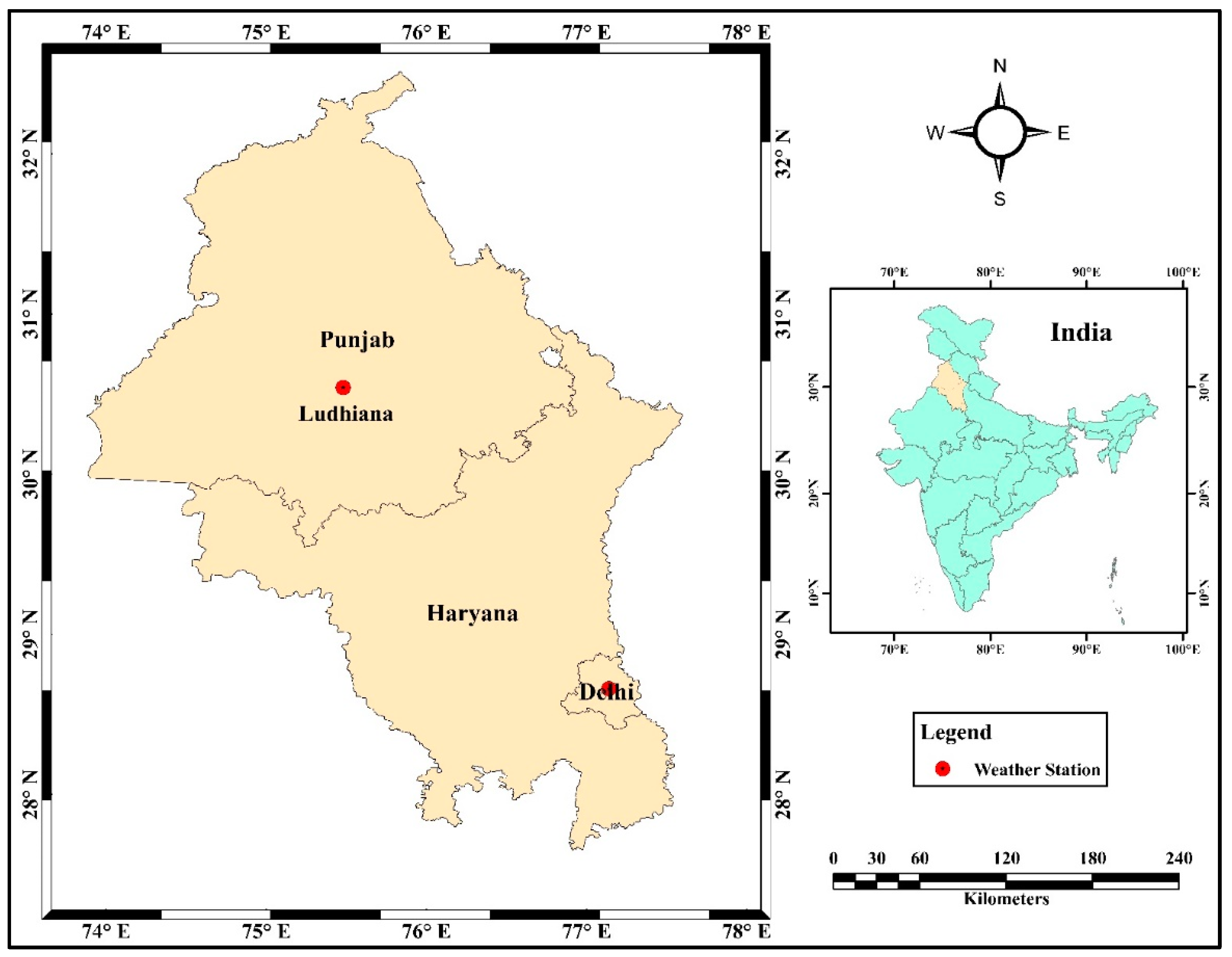
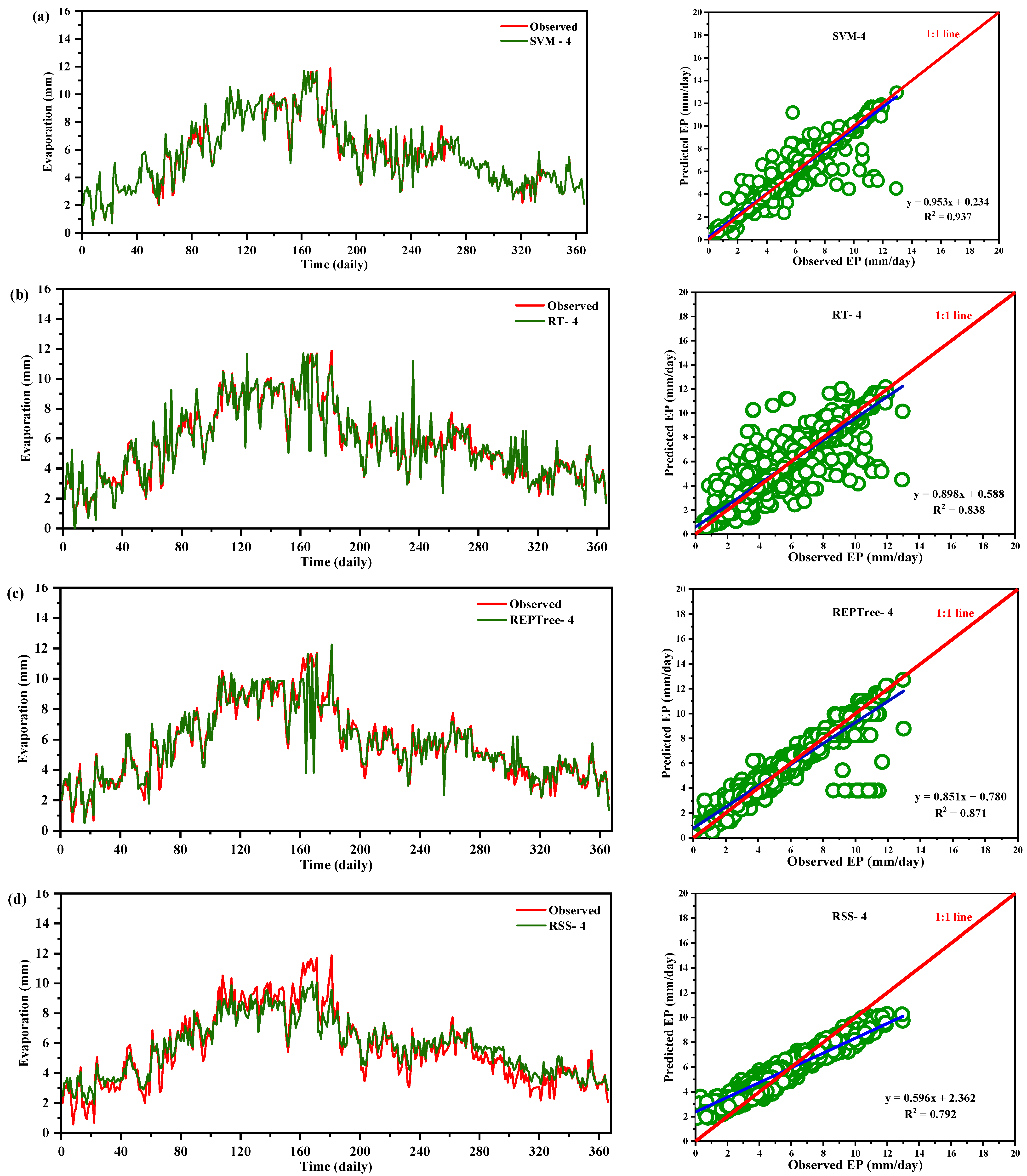
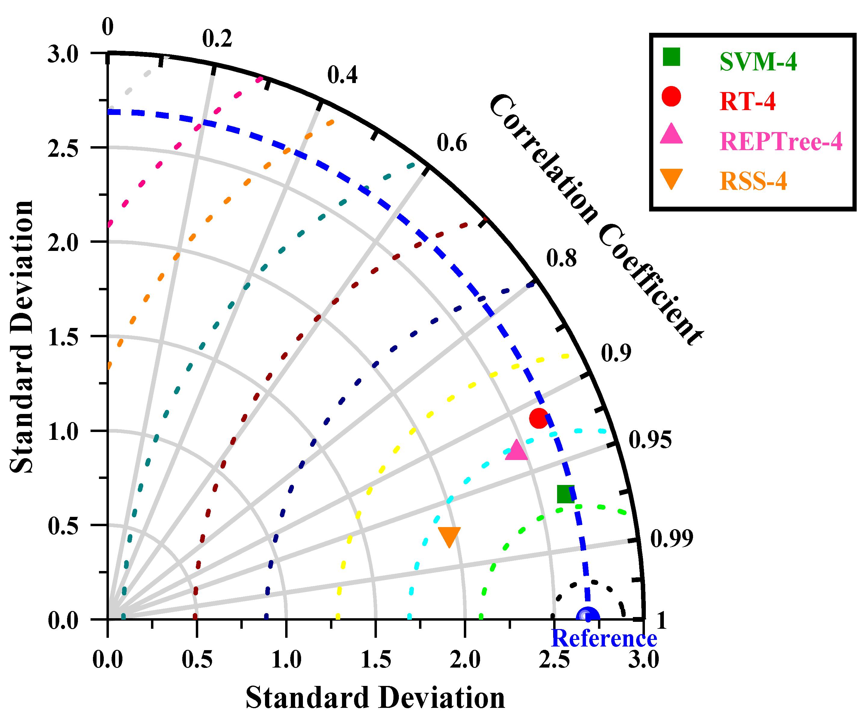
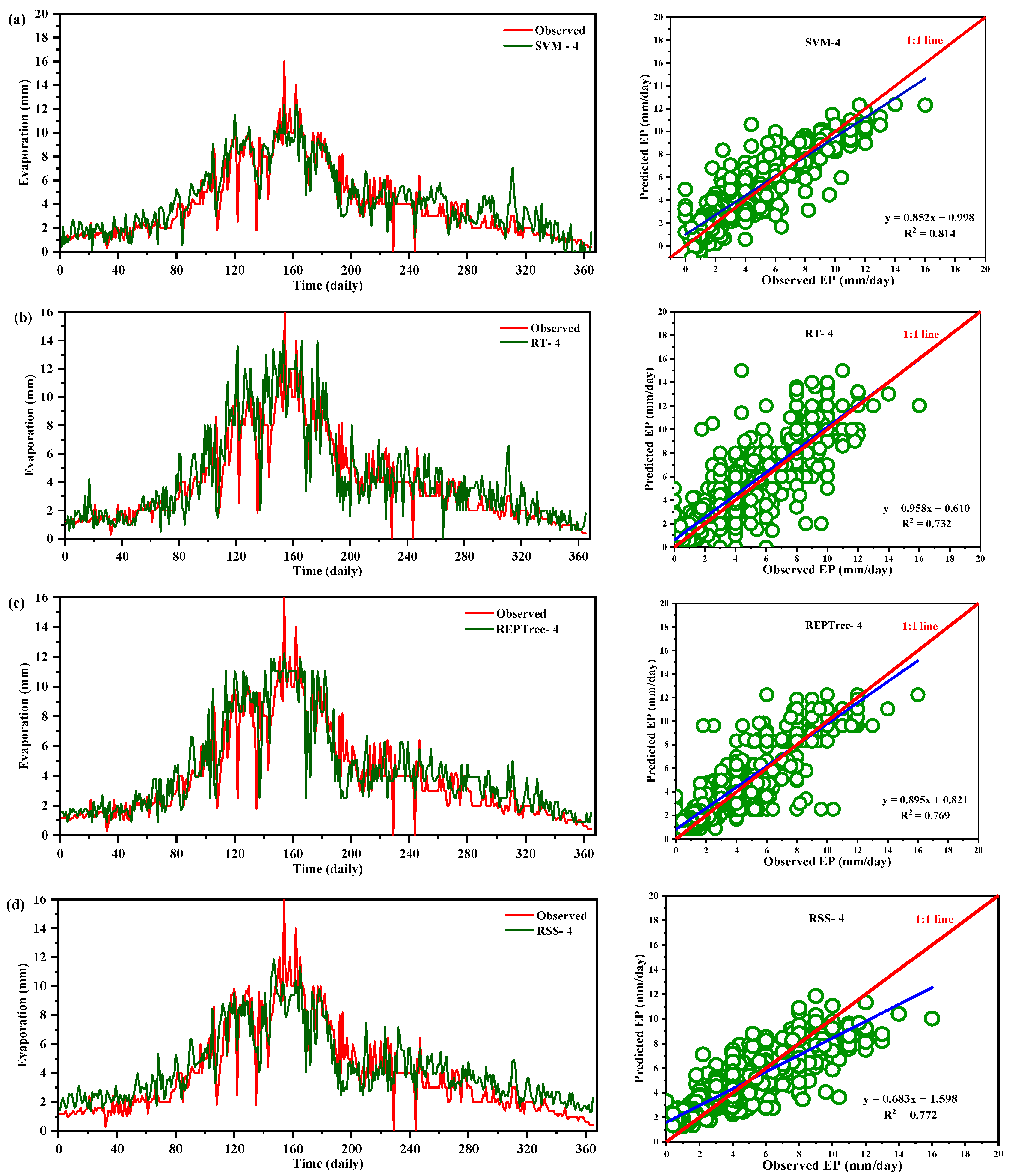
In the present state of soft computing wisdom, there are obscured or insufficient references to studies using meta-heuristics/artificial intelligence tools in the evaporation modeling in the Indian context especially covering the northern part. Thus, this study aims to evaluate and compare the predictability of four meta-heuristic algorithms, i.e., SVM, RT, REPTree, and RSS as predictive tools to estimate pan evaporation in two diverse agro-climate conditions in India. The predictive efficacies of the algorithms were compared in quantitative and qualitative terms to find the best candidate algorithm suitable for evaporation modeling for this region.

2. Materials and Methods

2.1. Research Area and Datasets

To carry out this research, the observed values of daily meteorological data, including pan evaporation, were collected and analyzed from the observatories at New Delhi and Ludhiana. Both stations are situated in semi-arid (New Delhi) and sub-humid (Ludhiana) agro-climatic regions in Northern India. Figure 1 depicts the locations of the chosen meteorological stations. The daily recorded climatic parameters including minimum–maximum temperatures (Tmin and Tmax, °C), wind speed (WS), relative humidity (RH), and sunshine hours (SSH) for the statistical period 1990–2020 (for New Delhi) and 2009–2019 (for Ludhiana), were obtained from respected meteorological organizations. Pan evaporation data were observed using the class A type pan (Figure 2). The detailed specification and climatic characteristics of the study locations are presented in

Table 1. Detailed description of the study stations.

Station	Time Span	Latitude, N	Longitude, E	MSL, m	Agro-Climatic Zone
New Delhi	1990–2020	28°38′2″ N	77°09′27″ E	228.61	Semi-arid
Ludhiana	2009–2019	30°54′00″ N	75°48′00″ E	247.00	Sub-humid

. The average annual rainfall at New Delhi and Ludhiana is 647 and 660 mm, respectively.

In the present study, the datasets were randomly grouped into two sections: training and testing subsets. Seventy-five per cent of the datasets were used for model training, with the remaining twenty-five per cent used for validating or testing the results of the models. Figure 3a,b shows the box–whisker plots of the meteorological parameters at two different stations. These box plots display data such as minimum, maximum, median, and quartile-wise values of meteorological parameters. The WEKA (version 3.8.5) developed at the University of Waikato, Waikato, New Zealand, is free software licensed under the General Public License (GNU) [23] was used in the present study to perform modelling.

2.2. Methodology

2.2.1. Best Subset Regression and Sensitivity Analysis

Selection of best input combinations is one of the most important stages for a soft computing model to forecast the engineering phenomena when there are many input variables. There are several approaches to specify the best combinations among all the possibilities, which includes best subset regression, mutual information, forward stepwise selection, etc. In the current study, the best subset regression analysis was performed to determine the best input combinations for modeling daily pan evaporation. The high temperature in the study regions is the basic predictor for pan evaporation. The sensitivity analysis was also performed to see the effects of the selected combination of meteorological variables in the performance of applied meta-heuristic algorithms.

2.2.2. Support Vector Machine

The support vector machine (SVM) is a supervised learning technique that was invented by Vapnik [24] and is used to address classification and regression issues. It was originally designed for classification difficulties. An optimization using a quadratic function is used to tackle the difficulty of learning new things. SVM determines the separating hyperplane that divides vector space into subsets of vectors for a given set of p-dimensional vectors in vector space; each separated subset (data set) is allocated to a single class for each set of p-dimensional vectors in vector space. The original SVM algorithm was created by Vladimir Vapnik and Alexey Chervonenk in 1963, and it is still in use today [24,25]. Nonlinear classifiers were suggested by Boser et al. [26], who recommended utilizing the kernel technique on maximum-margin hyperplanes to construct them. Cortes and Vapnik [25] proposed the current standard format (soft margin). Linear SVP is given in Equation (1):

$$x_1, y_1\dots \dots .x_n, y_n$$

(1)

where y₁ is either 1 or −1, depending on which class the point x₁ belongs to. Each x₁ represents a $\rho$-dimensional real vector. We need to identify the “maximum-margin hyperplane” that splits the group of points, x₁, where y₁ = 1 from the group of points where y₁ = −1, and is defined in such a way that the distance between the hyperplane and the closest point, x₁, in either group is maximized. Any hyperplane may be expressed mathematically as the set of points x fulfilling Equation (2):

$$w^{T}x-b=0$$

(2)

where x is the (non-normalized) normal vector to the hyperplane. This is similar to Hesse normal form, but x does not have to be a unit vector. The parameter $\frac{b}{\Vert w\parallel }$ specifies the hyperplane’s offset from the origin along the normal vector x. The graphic schematic layout and parameters selected for implementing the SVM algorithm are shown in Figure 4 and

Table 2. The parameters of the machine learning algorithm used for evaporation modeling.

Model Name	Description of Parameters
Support vector machine (SVM)	Kernel = normalized poly; batch size = 100, C = 1, regression optimizer = SMO improved; filter type = normalize training data; cache size = 250,000
Random tree (RT)	Batch size-100, seed = 1, minimum variance proportion = 0.001
Reduced error pruning tree (REPTree)	Batch size-100, Initial count = 0, number of folds = 3, random seed = 1, minimum proportion of the variance = 0.001, minimum number = 2, max depth = 1
Random subspace (RSS)	Batch size-100, classifier = REPTree, random seed-1, subspace size = 0. 5, numbers of executions slots = 1, number of iterations = 10

, respectively.

2.2.3. Random Tree

The random tree (RT) method is a supervised meta-heuristic that utilizes the bagging approach to generate random point data to construct a decision tree [27]. The model could tackle problems by forming an ensemble of predictors called the RT forest. It is a combination of RF and bagging techniques [28]. This algorithm had the ultimate advantage in that it constructs efficiently in both supervised and unsupervised learning and maintains accuracy even during complexity increases due to dynamic changes in the environment [29]. The parameters selected for implementing the RT algorithm are shown in Table 2.

2.2.4. Reduced Error Pruning Tree

The REPTree decision algorithm is a very rapid learning approach that produces a very low-error pruning tree. It constructs a regression tree and prunes it using back fitting with reduced error based on the data gain/variance [30]. The “reduce error pruning method” was used to minimize the difficulty of the model decision tree, resulting in a reduction in the number of errors caused by changes. Because of its easy setup, the decision tree technique is a popular method for categorizing issues [31]. For numeric characteristics, the algorithm only examines values once and it is basically the process of establishing a common set of decision-making instructions based on a forecaster variable quantity [32,33]. The REPTree procedure is a straightforward decision tree construction approach that use condensed error trimming to construct a regression tree using variance data [34] in case numerical ranges in the model have been established [35]. In this case, the execution of several knowledge algorithms in the WEKA environment is employed [36]. REPTree models are commonly applied in hydrological systems, surface runoff, and other disciplines. The REPTree model provides accurate results in a variety of fields such as ecological planning, flood susceptibility, soil erosion, climate, and hydrological processes, and it is very effectively applied in a variety of aspects such as irrigation planning, flood analysis, rainfall prediction, and evaporation, among others. This model has recently been employed in machine learning programming, and it is widely used by researchers and data scientists in Python programming. Table 2 shows the parameters that were chosen for use with this technique.

2.2.5. Random Subspace

Random subspace (RSS) is an ensemble algorithm that distributes a random subset of features to separate classifiers and then uses voting to aggregate their results [37]. RSS is especially advantageous when the number of training items is limited in comparison with the amount of data. Moreover, random subspace provides better classifiers than the original feature space when data presents many redundant features [38]. The subsets are randomly selected from classification training, with an integration of the number of classification rules [39]. The first step consists of a classification of initial space in subsets. Then, the results are obtained based on the majority of votes provided by:

$$\beta \left(x\right)=argma{x}_{y\in \left\{-1,1\right\}}{\displaystyle \sum }_d{\delta }_{sng}\left(C^b\left(x\right)\right),y$$

(3)

where δ is the Kronecker symbol, y ∈ {−1, 1} is a decision or class label of the classifier, and C^b(x) is the classification integration (C = 1, 2, …).

Table 2 shows the parameters that were chosen for use with this technique. The block diagram of RSS is shown in Figure 5. The simple algorithm of RSS is also trained in a parallel way [40]. More information about RSS and its implementations can be found in studies such as pan evaporation simulation [41] and reference evapotranspiration [40].

2.2.6. Meta-Heuristic Algorithms for Evaporation Modeling in Northern India

In the context of weather contingencies, often experienced in northern India, irrigation decisions were probably considered important to offset possible shifting of monsoon towards the northwest part of the country [42]. Therefore, evaporation estimation at finer resolution scale can be integrated into a sustainable irrigation plan for the entire region supporting any offset initiatives. The advent of high-resolution datasets of meteorological variables generated by Arias et al. [43] can be best translated into evaporation estimates for the northern region which falls in either of the agro-climatic conditions represented by the database stations. Though IPCC (Intergovernmental Panel on Climate Change) [43] has its own modeling criteria for evaporation modeling and reporting as a grid-based database, the candidate model proposed through this study can be more realistic representation of evaporation estimates over a large area.

2.3. Statistical Assessment and Validation

Throughout the investigation, pan evaporation (EP_d) measurement and predicted values were compared. Statistical assessment was done to compare the accuracy of the applied algorithms (i.e., SVM, RT, REPTree, and RSS) using the root mean square error (RMSE) [8,10,44], mean absolute error (MAE) [7,45], Nash–Sutcliffe efficiency (NSE) [4,45], Willmott index (WI) [8], and correlation coefficient (r) [19]. In addition, qualitative performance was evaluated through graphical scrutiny. The most accurate algorithm was selected based on the highest values of NSE, WI, and r while showing the lowermost values of MAE and RMSE among all selected meta-heuristic algorithms. All parameters are specified as follows: $E{P}_d{}_A^i$ is a recorded or actual value, $E{P}_d{}_P^i$ is a estimated or predicted value, ${\overline{EP}}_d{}_A^i$ and ${\overline{EP}}_d{}_p^i$ are the mean values of recorded and estimated samples, and N is the total number of selected samples.

2.3.1. Root Mean Square Error

The RMSE is the sample standard deviation of the variations between expected and actual values. It applies to the following formula:

$$\mathrm{RMSE}=\sqrt{\frac{1}{N}{{\displaystyle \sum }}_{i=1}^N{(E{P}_d{}_A^i-E{P}_d{}_P^i)}^2}$$

(4)

2.3.2. Mean Absolute Error (MAE)

The MAE evaluates the magnitude of mistakes in a sequence of predictions without taking into consideration their sign. It is a rough approximation of the absolute discrepancies between predicted and actual values throughout the test sample. It is defined as:

$$\mathrm{MAE}=\frac{1}{N}{{\displaystyle \sum }}_{i=1}^N|{\mathrm{ETo}}_P^i-{\mathrm{ETo}}_A^i|$$

(5)

2.3.3. Nash–Sutcliffe Efficiency

The Nash–Sutcliffe efficiency is the most commonly used model performance indicator. It ranges from 1 for perfect fit to negative infinity. The value of 0 indicates that the mean value produced the same level of accuracy.

$$\mathrm{NSE}=1-\left[\frac{{{\displaystyle \sum }}_{i=1}^N{(E{P}_d{}_A^i-E{P}_d{}_P^i)}^2}{{{\displaystyle \sum }}_{i=1}^N{(E{P}_d{}_A^i-{\overline{EP}}_d{}_A^i)}^2}\right]$$

(6)

2.3.4. Willmott Index

The Willmott index (WI) is also called the index of agreement. The WI ranges from zero to one (0 < WI < 1); approximately 1 is the ideal agreement/fit.

$$\mathrm{WI}=1-\frac{{{\displaystyle \sum }}_{i=1}^N{(E{P}_d{}_A^i-E{P}_d{}_P^i)}^2}{{{\displaystyle \sum }}_{i=1}^N{\left(\left|E{P}_d{}_P^i-{\overline{EP}}_d{}_A^i\right|+\left|E{P}_d{}_A^i-{\overline{EP}}_d{}_A^i\right|\right)}^2}$$

(7)

2.3.5. Correlation Coefficient

The correlation coefficient (r) measures how well the model matches experimental data. It is defined as:

$$\mathrm{r}=\frac{{{\displaystyle \sum }}_{i=1}^N\left(E{P}_d{}_A^i-{\overline{EP}}_d{}_A^i\right)\left(E{P}_d{}_P^i-{\overline{EP}}_d{}_P^i\right)}{\sqrt{{{\displaystyle \sum }}_{i=1}^N{\left(E{P}_d{}_A^i-{\overline{EP}}_d{}_A^i\right)}^2{{\displaystyle \sum }}_{i=1}^N{\left(E{P}_d{}_P^i-{\overline{EP}}_d{}_P^i\right)}^2}}$$

(8)

3. Results

3.1. Best Subset Regression and Sensitivity Analysis

3.1.1. Selection of Best Input Combination

In modeling, the assortment of best input parameters is an important step for the best performance of the selected models. Different combinations of meteorological parameters were used for the selection of the best input combination. In the present study, five combinations were tested as presented in

Table 3. The best subset regression analysis for determining the best input combinations at the New Delhi station.

No. of Variables	Variables	MSE	R2	Adjusted R2	Mallows’ Cp	Akaike’s AIC	Schwarz’s SBC	Amemiya’s PC
1	RH	4.140	0.558	0.558	5595.888	5709.171	5721.768	0.442
2	Tmin/RH	2.245	0.760	0.760	1199.073	3252.387	3271.282	0.240
3	Tmin/RH/WS	1.899	0.797	0.797	396.790	2580.839	2606.032	0.203
4	Tmin/RH/SSH/WS	1.748	0.813	0.813	46.783	2248.347	2279.838	0.187
5	Tmin/Tmax/RH/SSH/WS	1.730	0.815	0.815	6.000	2207.727	2245.517	0.185

and

Table 4. The best subset regression analysis for determining the best input combinations at the Ludhiana station.

No. of Variables	Variables	MSE	R2	Adjusted R2	Mallows’ Cp	Akaike’s AIC	Schwarz’s SBC	Amemiya’s PC
1	Tmax	3.316	0.574	0.574	35,687.061	13,574.801	13,589.470	0.426
2	Tmin/RH	1.602	0.794	0.794	11,389.501	5337.900	5359.903	0.206
3	Tmin/RH/WS	0.903	0.884	0.884	1488.456	−1147.456	−1118.118	0.116
4	Tmin/RH/SSH/WS	0.800	0.897	0.897	21.311	−2525.511	−2488.838	0.103
5	Tmin/Tmax/RH/SSH/WS	0.799	0.897	0.897	6.000	−2540.818	−2496.810	0.103

. The best input combination has been selected using the six statistical criteria, i.e., MSE, determination coefficients (R2), adjusted R2, Mallows’ Cp, Akaike’s AIC, and Amemiya’s PC at two stations in northern India and the results are shown in Table 3 and Table 4. From Table 3, it can be seen that the bold blue row is identified as the best input combination as it has the lowest values of Mallows’ Cp of 21.31, Amemiya’s PC of 0.103, and the highest value of R2 (0.0.897) and high Adj-R² (0.897) among all input combinations at the New Delhi station. Similarly, at the Ludhiana station, the bold blue row identified as the best input combination with the lowest values of Mallows’ Cp of 46.78, Amemiya’s PC of 0.187, and highest value of R2 (0.813) and high Adj-R² (0.813) among all the input combinations (Table 4). The correlation matrix showing variable correlations used in the study exhibits significantly higher correlations with the dependent variable EP_d (Figure 6). The complete datasets for both the stations are divided into two segments: training dataset and testing dataset (Table 1). The whole data set were spilt into two sets comprising 75% of datasets for training and the remaining 25% for validating the models.

3.1.2. Sensitivity Analysis

The performance of the models is highly influenced by combinations of the input variables. Some have positive and others can have a negative contributions to the accuracy of the selected model. The selection of the best influential variables was done through sensitivity analysis to get the best performance of models in the prediction of daily pan evaporation at two meteorological stations. The obtained results from the regression analysis can be seen in

Table 5. The regression analysis for identifying the most effective parameters for evaporation estimation at the New Delhi station.

Source	Value	Standard Error	t	Pr > |t|	Lower Bound (95%)	Upper Bound (95%)
Tmin	0.404	0.003	124.203	<0.0001	0.398	0.410
Tmax	0.000	0.000
RH	−0.516	0.004	144.715	<0.0001	−0.523	−0.509
SSH	0.132	0.003	38.302	<0.0001	0.125	0.139
WS	0.336	0.003	99.209	<0.0001	0.329	0.342

and

Table 6. The regression analysis for identifying the most effective parameters for evaporation estimation at the Ludhiana station.

Source	Value	Standard Error	t	Pr > |t|	Lower Bound (95%)	Upper Bound (95%)
Tmin	0.393	0.007	52.583	<0.0001	0.378	0.407
Tmax	0.000	0.000
RH	−0.533	0.008	65.534	<0.0001	−0.549	−0.517
SSH	0.147	0.008	18.665	<0.0001	0.132	0.162
WS	0.223	0.007	30.111	<0.0001	0.209	0.238

, and Figure 7 and Figure 8. The results of regression analysis on all input parameters showed that Tmin, RH, SSH, and WS by having absolute standard coefficients (0.404, −0.516, 0.132, and 0.336) were identified as the most influential input parameters, respectively, for estimation of pan evaporation at the New Delhi station. Similarly, for the Ludhiana station, the findings of regression analysis on all input parameters revealed that Tmin, RH, SSH, and WS by having the highest standard coefficients (0.393, −0.533, 0.147, and 0.223) were identified as the most influential input parameters, respectively.

3.2. Implementation of Meta-Heuristics Algorithm for Daily EP Estimation

The pan evaporation at two different stations was estimated by applying four machine learning algorithms (i.e., SVM, RT, REPTree, and RSS). The performances of the applied algorithms were evaluated and compared based on performance indicators (i.e., MAE, RMSE, NSE, WI, and r). The model with a high value of NSE, WI, and r close to 1 and the lowest value of MAE and RMSE with close to 0 is considered the higher accuracy in the estimation of pan evaporation. The general trend of MAE, RMSE, NSE, WI, and r is presented in

Table 7. RMSE, NSE, WI, and r for meta-heuristic algorithms-based models during the training and testing phase at the New Delhi station.

Machine Learning Algorithm	Training					Testing
	MAE	RMSE	NSE	WI	r	MAE	RMSE	NSE	WI	r
SVM-4	0.314	0.968	0.877	0.968	0.938	0.055	0.092	0.937	0.984	0.968
RT-4	0.034	0.080	0.999	0.999	0.999	0.554	1.544	0.834	0.956	0.915
REPTree-4	0.526	0.898	0.894	0.971	0.945	0.518	1.455	0.754	0.922	0.933
RSS-4	0.779	1.053	0.854	0.952	0.939	0.781	1.497	0.739	0.901	0.890

and

Table 8. RMSE, NSE, WI, and r for meta-heuristic algorithms-based models during the training and testing phase at the Ludhiana station.

Machine Learning Algorithm	Training					Testing
	MAE	RMSE	NSE	WI	r	MAE	RMSE	NSE	WI	r
SVM-4	0.961	1.325	0.816	0.946	0.903	0.993	1.317	0.795	0.943	0.902
RT-4	0.039	0.086	0.999	0.999	0.998	1.220	1.814	0.641	0.914	0.856
REPTree-4	0.735	1.070	0.880	0.967	0.938	1.045	1.509	0.731	0.930	0.876
RSS-4	0.968	1.330	0.814	0.935	0.923	1.118	1.448	0.752	0.917	0.878

. The SVM-4 model has the potential to estimate the pan evaporation with greater accuracy as compared with other algorithms at both stations.

3.2.1. Estimation of Pan Evaporation at New Delhi Station

The performance of applied algorithms, namely, SVM, RT, REPTree, and RSS was assessed employing performance indicators (i.e., MAE, RMSE, NSE, WI, and r) at the New Delhi station and presented in Table 7. It is evident from the table that the random tree-4 (RT-4) model performed better during the training period and the support vector machine-4 (SVM-4) models performed better than other applied algorithms during the testing period. Therefore, the values of NSE, WI, and correlation coefficient (r) were highest and error parameters (i.e., MAE and RSME) were obtained lowest for the SVM-4 model compared with the other models during the testing span and considered as the best model in daily EP estimation at the New Delhi station.

Figure 9 displays the temporal fluctuation between estimated and observed daily EP values, as well as associated scatter plots (a to d). The regression line yielded coefficients of determination (R2) of 0.937 for the SVM-4, 0.838 for the RT-4 model, 0.871 for the REPTree-4 model, and 0.792 for the RSS-4 models in scatter plots, respectively. The SVM-4 model showed the regression line close to the best-fit line and showed superior performance among other models. It is also observed that the performances of the applied models were slightly superior at the New Delhi station than the Ludhiana station.

A radar map of the performance indicators was used to measure the performance of the applied models in addition to the aforementioned models. The values of performance indicators are given in Figure 10 to provide a better diagnostic study of the efficiency of all models. It is obvious from the illustrations of the figures that the SVM-4 model has a lower MAE and RMSE value, and a higher NSE, WI, and Pearson’s r value than the other models. Consequently, it was discovered that the SVM-4 model outperformed the other models. Further comparative analysis of models was done using the Taylor diagram (Figure 11). Based on the standard deviation, correlation, and root mean square error, the SVM-4 model was found to be the closest to the observed location, while the RT-4 model was found to be the furthest. This showed RT-4 as the worst model and SVM-4 as the best model among the selected models.

3.2.2. Estimation of Pan Evaporation at Ludhiana Station

Table 8 displays the results of the daily EP estimation at the Ludhiana station, as derived from the station’s data. It revealed that the RT-4 model was superior with a high value of correlation coefficient (r) = 0.998, NSE = 0.999, WI = 0.999, and lower values of MAE = 0.039 mm/day and RMSE = 0.086, mm/day in the training period. Whereas, the SVM-4 model showed superiority among other models during the testing period with r = 0.902, NSE = 0.795, WI = 0.943, MAE = 0.993 mm/day, and RMSE = 1.317 mm/day. Therefore, it revealed that the SVM-4 model performs superior to the applied models.

As shown in Figure 12a–d, each of the SVM, RT, REPTree, and RSS models produced time series and scatter plots comparing predicted daily EP to their observed daily EP throughout the testing period, respectively. The R2 was assessed using the regression line and was found to be 0.814 for the SVM-4 model, 0.732 for the RT-4 model, 0.769 for the REPTree-4 model, and 0.772 for the RSS-4 model, according to the results. The RL of the SVM-4 model is located near the best fit 1:1 line. This reveals that the SVM-4 model has high accuracy in the estimation of daily EP at the Ludhiana station.

The comparison among the applied models was made using a radar chart of MAE, RMSE, NSE, WI, and Pearson’s r values. Performance indicators were shown by a radar chart in Figure 13, which displayed the best-calculated values of the indicators. It is obvious from the figure that the SVM-4 model has the best values for all of the performance metrics measured. According to Figure 14, a further comparative examination of the models’ was performed via the use of the Taylor diagram to compare the models’ performances. According to the graph, the SVM-4 model is the one that is closest to the observed point, followed by the REPTree-4 and RSS-4 models, which are based on the standard deviation, correlation, and RMSE. The SVM-4 model outperformed the RT-4 model in the prediction of EP_d at the Ludhiana station.

Machine learning algorithms were tested for their accuracy in estimating daily EP (EP_d) at two meteorological stations, and their performance was evaluated. The findings suggest that the applied meta-heuristic approaches have predictive capabilities in daily EP estimation. The SVM-4 model was comparatively more promising over the other applied models. The time series and scatter plots between the observed and estimated EPd at two meteorological stations are displayed in Figure 9 and Figure 10. In both the stations, the SVM-4 was found to perform better statistically over the other models. This establishes the superior capabilities of the SVM-4 model in daily EP prediction. Further comparison between algorithms was made using a radar chart (Figure 11) of performance indicators and the result revealed that the SVM-4 model predicted precisely EP_d values for both stations with least MAE and RMSE. The Taylor diagram (Figure 12 and Figure 13) also depicted a comparable performance in daily EP values for all the models. Based on the standard deviation, correlation, and RMSE, the RT-4 model was found to be the furthest, while the SVM-4 model was found to be the closest to the observed data at both meteorological stations. This again confirms the precedence of SVM algorithm in daily EP prediction compared with other selected algorithms.

4. Discussion

The results obtained from the present study were also validated with other recent work [2,8,19,46] conducted across different continents of the world. Al-Mukhtar [12] evaluated two different machine learning techniques (i.e., SVM and backpropagation network) in the estimation of daily evaporation values. Results revealed that applied SVM machine learning algorithms offer great ability to predict the daily pan evaporation values and can be used as a promising alternative for pan evaporation estimation. The accuracy of five machine learning methods (i.e., MARS, multi-model artificial neural network (MM-ANN), SVM, multi-gene genetic programming (MGGP), and M5Tree) to predict the monthly pan evaporation in India was evaluated by Malik et al. [2] which also revealed a similar outcome with SVM being more prolific. In this study, they observed that the MM-ANN and MGGP algorithms had superior prediction performance when compared with the MARS and SVM algorithms, as well as the M5Tree method, as shown by their high levels of RMSE. Tezel and Buyukyildiz [18] evaluated the ANN, radial basis function network (RBFN), and SVM machine learning algorithm approaches for monthly pan evaporation at the Beysehir meteorological observatory, which is situated in Turkey’s southwestern region. Based on the performance indicators selected in the study, both the algorithms ANN and ɛ-SVM produced similar results. Chen et al. [19] investigated the performance of SVM for the prediction of monthly pan evaporation at six different stations located in the Yangtze River basin of China. The study concluded that the SVM techniques showed superiority over the traditional methods for estimating pan evaporation. The present study also confirmed that the SVM machine learning algorithm has higher accuracy than other applied algorithms in the prediction of daily pan evaporation (EP_d) in diverse agro-climatic settings.

5. Conclusions

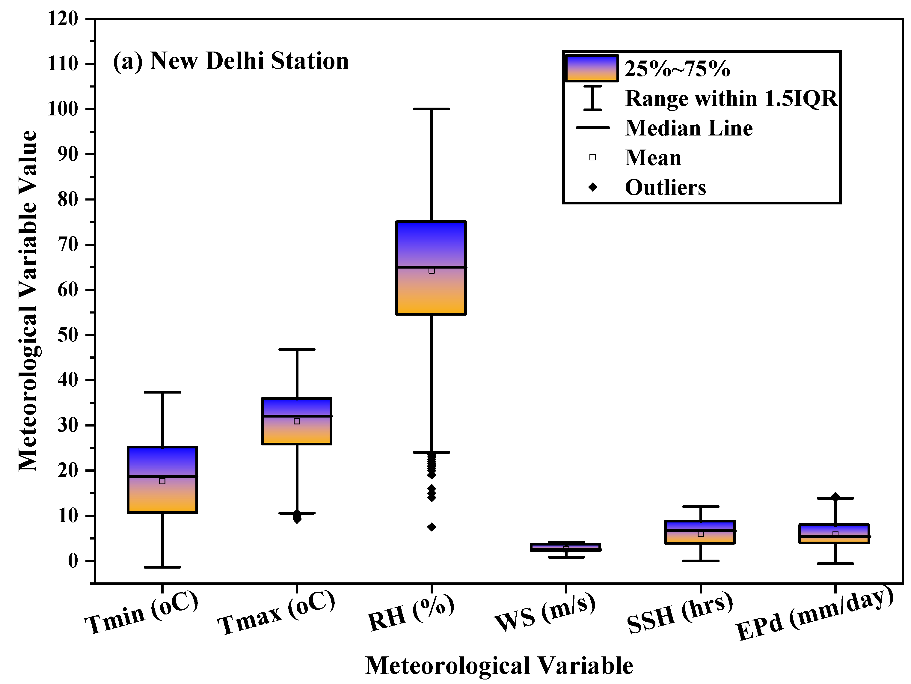
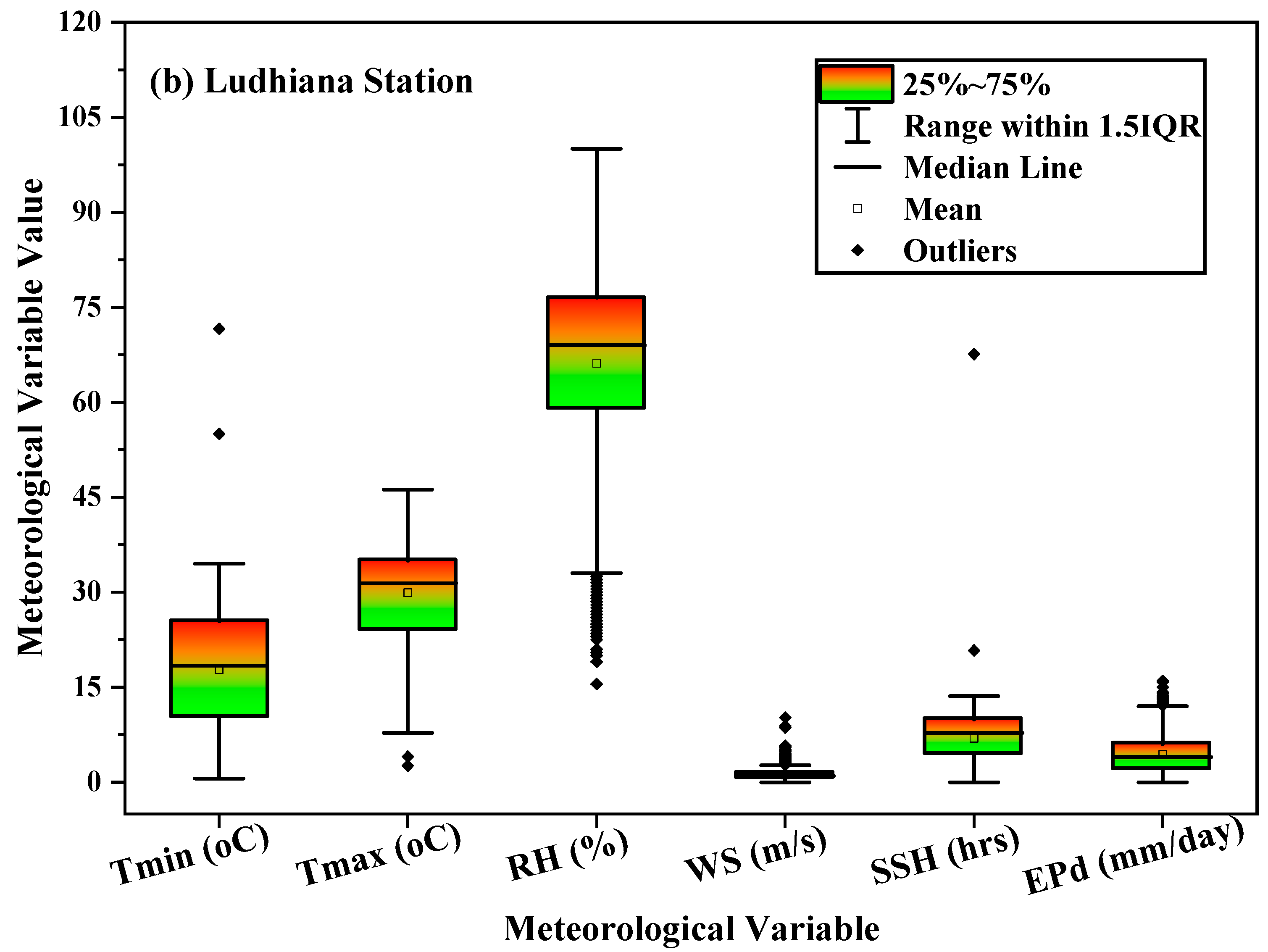
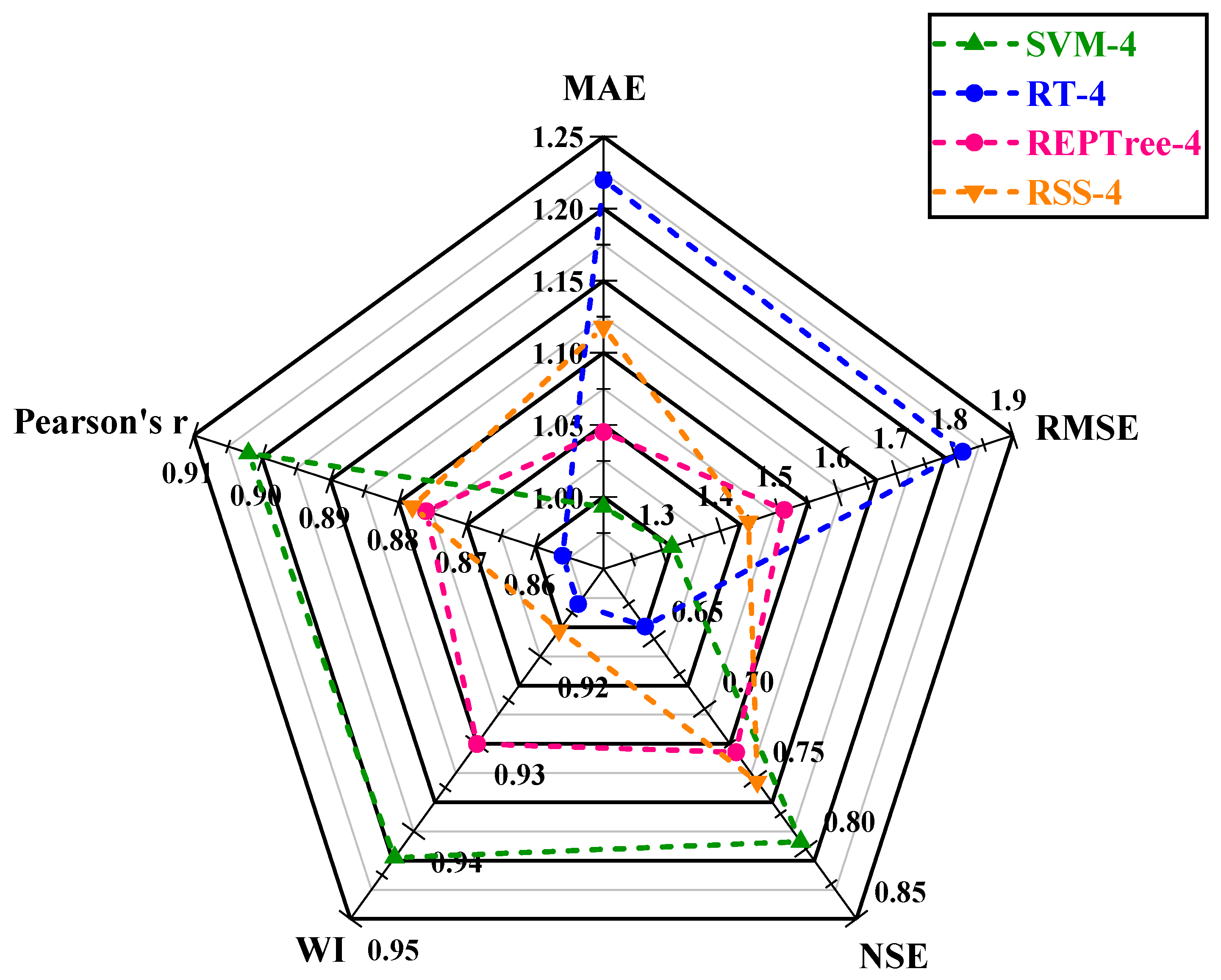
This study evaluated the potential of meta-heuristic approaches in forecasting daily pan evaporation (EP_d) at two different meteorological stations. Four models were developed: support vector machine (SVM), random tree (RT), reduced error pruning tree (REPTree), and random subspace (RSS). Furthermore, the assortment and influence of input combinations on the performance of the meta-heuristic algorithms in EP_d prediction were carried out through regression and sensitivity analysis. The results of regression analysis on all input parameters showed that Tmin, RH, SSH, and WS, by having absolute standard coefficients (0.404/0.393, −0.516/−0.533, 0.132/0.147, and 0.336/0.223), were identified as the most influential input parameters at the New Delhi and Ludhiana stations, respectively. The performance of applied models was assessed using well-known performance indicators (i.e., MAE. RMSE, NSE, WI, and r) and interpreting the visual graphics. The SVM algorithm outperformed the other applied algorithms during the testing period and is consistent over the two locations tested representing two diverse climatic zones of India and mostly covering the northern region. Thus, SVM algorithms may be adopted for the estimation of daily pan evaporation in the selected two different climatic conditions. Overall, the developed methodology allows prediction with a model trained on the available meteorological data as input, which could be an interesting tool for irrigation engineers, hydrologists, and environmentalists for irrigation scheduling and sustainable management of available water resources.

References

1. Ghorbani, M.A.; Jabehdar, M.A.; Yaseen, Z.M.; Inyurt, S. Solving the pan evaporation process complexity using the development of multiple mode of neurocomputing models. Theor. Appl. Clim. 2021, 145, 1521–1539. [Google Scholar] [CrossRef]
2. Malik, A.; Kumar, A.; Kim, S.; Kashani, M.H.; Karimi, V.; Sharafati, A.; Ghorbani, M.A.; Al-Ansari, N.; Salih, S.Q.; Yaseen, Z.M.; et al. Modeling monthly pan evaporation process over the Indian central Himalayas: Application of multiple learning artificial intelligence model. Eng. Appl. Comput. Fluid Mech. 2020, 14, 323–338. [Google Scholar] [CrossRef] [Green Version]
3. Kushwaha, N.L.; Bhardwaj, A.; Verma, V.K. Hydrologic Response of Takarla-Ballowal Watershed in Shivalik Foot-Hills Based on Morphometric Analysis Using Remote Sensing and GIS. J. Indian Water Resour. Soc. 2016, 36, 17–25. [Google Scholar]
4. Alsumaiei, A.A. Utility of Artificial Neural Networks in Modeling Pan Evaporation in Hyper-Arid Climates. Water 2020, 12, 1508. [Google Scholar] [CrossRef]
5. Malik, A.; Rai, P.; Heddam, S.; Kisi, O.; Sharafati, A.; Salih, S.; Al-Ansari, N.; Yaseen, Z. Pan Evaporation Estimation in Uttarakhand and Uttar Pradesh States, India: Validity of an Integrative Data Intelligence Model. Atmosphere 2020, 11, 553. [Google Scholar] [CrossRef]
6. Kisi, O.; Heddam, S. Evaporation modelling by heuristic regression approaches using only temperature data. Hydrol. Sci. J. 2019, 64, 653–672. [Google Scholar] [CrossRef]
7. Elbeltagi, A.; Aslam, M.R.; Mokhtar, A.; Deb, P.; Abubakar, G.A.; Kushwaha, N.; Venancio, L.P.; Malik, A.; Kumar, N.; Deng, J. Spatial and temporal variability analysis of green and blue evapotranspiration of wheat in the Egyptian Nile Delta from 1997 to 2017. J. Hydrol. 2021, 594, 125662. [Google Scholar] [CrossRef]
8. Kumar, M.; Kumari, A.; Kumar, D.; Al-Ansari, N.; Ali, R.; Kumar, R.; Kumar, A.; Elbeltagi, A.; Kuriqi, A. The Superiority of Data-Driven Techniques for Estimation of Daily Pan Evaporation. Atmosphere 2021, 12, 701. [Google Scholar] [CrossRef]
9. Penman, H.L.; Keen, B.A. Natural Evaporation from Open Water, Bare Soil and Grass. Proceedings of the Royal Society of London. Series A. Math. Phys. Sci. 1948, 193, 120–145. [Google Scholar] [CrossRef] [Green Version]
10. Ghorbani, M.A.; Deo, R.C.; Yaseen, Z.M.; Kashani, M.H.; Mohammadi, B. Pan evaporation prediction using a hybrid multilayer perceptron-firefly algorithm (MLP-FFA) model: Case study in North Iran. Theor. Appl. Clim. 2018, 133, 1119–1131. [Google Scholar] [CrossRef]
11. Kim, S.; Singh, V.P.; Seo, Y. Evaluation of pan evaporation modeling with two different neural networks and weather station data. Theor. Appl. Clim. 2013, 117, 1–13. [Google Scholar] [CrossRef]
12. Al-Mukhtar, M. Modeling of pan evaporation based on the development of machine learning methods. Theor. Appl. Clim. 2021, 146, 961–979. [Google Scholar] [CrossRef]
13. Guan, Y.; Mohammadi, B.; Pham, Q.B.; Adarsh, S.; Balkhair, K.S.; Rahman, K.U.; Linh, N.T.T.; Tri, D.Q. A novel approach for predicting daily pan evaporation in the coastal regions of Iran using support vector regression coupled with krill herd algorithm model. Theor. Appl. Clim. 2020, 142, 349–367. [Google Scholar] [CrossRef]
14. Rahimikhoob, A. Estimating daily pan evaporation using artificial neural network in a semi-arid environment. Theor. Appl. Clim. 2009, 98, 101–105. [Google Scholar] [CrossRef]
15. Yaseen, Z.M.; Sulaiman, S.O.; Deo, R.C.; Chau, K.-W. An enhanced extreme learning machine model for river flow forecasting: State-of-the-art, practical applications in water resource engineering area and future research direction. J. Hydrol. 2019, 569, 387–408. [Google Scholar] [CrossRef]
16. Adnan, R.; Heddam, S.; Yaseen, Z.; Shahid, S.; Kisi, O.; Li, B. Prediction of Potential Evapotranspiration Using Temperature-Based Heuristic Approaches. Sustainability 2020, 13, 297. [Google Scholar] [CrossRef]
17. Tabari, H.; Grismer, M.E.; Trajkovic, S. Comparative analysis of 31 reference evapotranspiration methods under humid conditions. Irrig. Sci. 2013, 31, 107–117. [Google Scholar] [CrossRef]
18. Tezel, G.; Buyukyildiz, M. Monthly evaporation forecasting using artificial neural networks and support vector machines. Theor. Appl. Clim. 2016, 124, 69–80. [Google Scholar] [CrossRef]
19. Chen, J.-L.; Yang, H.; Lv, M.-Q.; Xiao, Z.-L.; Wu, S.J. Estimation of monthly pan evaporation using support vector machine in Three Gorges Reservoir Area, China. Theor. Appl. Clim. 2019, 138, 1095–1107. [Google Scholar] [CrossRef]
20. Deo, R.C.; Samui, P.; Kim, D. Estimation of monthly evaporative loss using relevance vector machine, extreme learning machine and multivariate adaptive regression spline models. Stoch. Environ. Res. Risk Assess. 2016, 30, 1769–1784. [Google Scholar] [CrossRef]
21. Pammar, L.; Deka, P.C. Daily pan evaporation modeling in climatically contrasting zones with hybridization of wavelet transform and support vector machines. Paddy Water Environ. 2017, 15, 711–722. [Google Scholar] [CrossRef]
22. Ghaderpour, E.; Vujadinovic, T.; Hassan, Q.K. Application of the Least-Squares Wavelet software in hydrology: Athabasca River Basin. J. Hydrol. Reg. Stud. 2021, 36, 100847. [Google Scholar] [CrossRef]
23. Garner, S.R. Weka: The Waikato Environment for Knowledge Analysis. In Proceedings of the New Zealand Computer Science Research Students Conference, Waikato, New Zealand, 18–21 April 1995; pp. 57–64. [Google Scholar]
24. Sain, S.R.; Vapnik, V.N. The Nature of Statistical Learning Theory. Technometrics 1996, 38, 409. [Google Scholar] [CrossRef]
25. Cortes, C.; Vapnik, V. Support-vector networks. Mach. Learn. 1995, 20, 273–297. [Google Scholar] [CrossRef]
26. Boser, B.E.; Guyon, I.M.; Vapnik, V.N. A training algorithm for optimal margin classifiers. In Proceedings of the Fifth Annual Workshop on Computational Learning Theory, Pittsburgh, PA, USA, 27–29 July 1992; Association for Computing Machinery: New York, NY, USA, 1992; pp. 144–152. [Google Scholar]
27. Khosravi, K.; Daggupati, P.; Alami, M.T.; Awadh, S.M.; Ghareb, M.I.; Panahi, M.; Pham, B.T.; Rezaie, F.; Qi, C.; Yaseen, Z.M. Meteorological data mining and hybrid data-intelligence models for reference evaporation simulation: A case study in Iraq. Comput. Electron. Agric. 2019, 167, 105041. [Google Scholar] [CrossRef]
28. Cutler, A.; Cutler, D.R.; Stevens, J.R. Random Forests. In Ensemble Machine Learning: Methods and Applications; Zhang, C., Ma, Y., Eds.; Springer: Boston, MA, USA, 2012; pp. 157–175. ISBN 978-1-4419-9326-7. [Google Scholar]
29. Mu, X.; Ting, K.M.; Zhou, Z.-H. Classification Under Streaming Emerging New Classes: A Solution Using Completely-Random Trees. IEEE Trans. Knowl. Data Eng. 2017, 29, 1605–1618. [Google Scholar] [CrossRef] [Green Version]
30. Joseph, K.S.; Ravichandran, T. A Comparative Evaluation of Software Effort Estimation Using REPTree and K* in Handling with Missing Values. Aust. J. Basic Appl. Sci. 2012, 6, 312–317. [Google Scholar]
31. Verbyla, D.L. Classification trees: A new discrimination tool. Can. J. For. Res. 1987, 17, 1150–1152. [Google Scholar] [CrossRef]
32. Bharti, B.; Pandey, A.; Tripathi, S.K.; Kumar, D. Modelling of runoff and sediment yield using ANN, LS-SVR, REPTree and M5 models. Hydrol. Res. 2017, 48, 1489–1507. [Google Scholar] [CrossRef]
33. Breiman, L.; Friedman, J.H.; Olshen, R.A.; Stone, C.J. Classification and Regression Trees; CRC Press: Boca Raton, FL, USA, 2017; ISBN 9781315139470. [Google Scholar]
34. Kumar, A.R.S.; Ojha, C.S.P.; Goyal, M.K.; Singh, R.D.; Swamee, P.K. Modeling of Suspended Sediment Concentration at Kasol in India Using ANN, Fuzzy Logic, and Decision Tree Algorithms. J. Hydrol. Eng. 2012, 17, 394–404. [Google Scholar] [CrossRef]
35. Daud, N.R.; Corne, D.W. Human Readable Rule Induction in Medical Data Mining. In Proceedings of the European Computing Conference; Mastorakis, N., Mladenov, V., Kontargyri, V.T., Eds.; Springer: Boston, MA, USA, 2009; pp. 787–798. [Google Scholar]
36. Witten, I.H.; Frank, E. Practical Machine Learning Tools and Techniques with Java Implementations. ACM Sigmod Rec. 2002, 31, 76–77. [Google Scholar] [CrossRef]
37. Ho, T.K. The random subspace method for constructing decision forests. IEEE Trans. Pattern Anal. Mach. Intell. 1998, 20, 832–844. [Google Scholar] [CrossRef] [Green Version]
38. Skurichina, M.; Duin, R.P.W. Bagging, Boosting and the Random Subspace Method for Linear Classifiers. Pattern Anal. Appl. 2002, 5, 121–135. [Google Scholar] [CrossRef]
39. Kuncheva, L.I.; Plumpton, C.O. Choosing Parameters for Random Subspace Ensembles for FMRI Classification. In International Workshop on Multiple Classifier Systems; Springer: Berlin/Heidelberg, Germany, 2010; pp. 54–63. [Google Scholar]
40. Salam, R.; Islam, A.R.M.T. Potential of RT, bagging and RS ensemble learning algorithms for reference evapotranspiration prediction using climatic data-limited humid region in Bangladesh. J. Hydrol. 2020, 590, 125241. [Google Scholar] [CrossRef]
41. Shabani, S.; Samadianfard, S.; Sattari, M.T.; Mosavi, A.; Shamshirband, S.; Kmet, T.; Várkonyi-Kóczy, A.R. Modeling Pan Evaporation Using Gaussian Process Regression K-Nearest Neighbors Random Forest and Support Vector Machines; Comparative Analysis. Atmosphere 2020, 11, 66. [Google Scholar] [CrossRef] [Green Version]
42. Devanand, A.; Huang, M.; Ashfaq, M.; Barik, B.; Ghosh, S. Choice of Irrigation Water Management Practice Affects Indian Summer Monsoon Rainfall and Its Extremes. Geophys. Res. Lett. 2019, 46, 9126–9135. [Google Scholar] [CrossRef]
43. Arias, P.; Bellouin, N.; Coppola, E.; Jones, R.; Krinner, G.; Marotzke, J.; Naik, V.; Palmer, M.; Plattner, G.-K.; Rogelj, J.; et al. Climate Change 2021: The Physical Science Basis. Contribution of Working Group14 I to the Sixth Assessment Report of the Intergovernmental Panel on Climate Change. Technical Summary; Masson-Delmotte, V., Zhai, P., Pirani, A., Conners, S.L., Péan, C., Berger, S., Caud, N., Chen, Y., Goldfarb, L., Gomis, M.I., et al., Eds.; Cambridge University Press: Cambridge, UK, 2021. [Google Scholar]
44. Sarwar, A.; Peters, R.T.; Mohamed, A.Z. Linear mixed modeling and artificial neural network techniques for predicting wind drift and evaporation losses under moving sprinkler irrigation systems. Irrig. Sci. 2019, 38, 177–188. [Google Scholar] [CrossRef]
45. Malik, A.; Tikhamarine, Y.; Al-Ansari, N.; Shahid, S.; Sekhon, H.S.; Pal, R.K.; Rai, P.; Pandey, K.; Singh, P.; Elbeltagi, A.; et al. Daily pan-evaporation estimation in different agro-climatic zones using novel hybrid support vector regression optimized by Salp swarm algorithm in conjunction with gamma test. Eng. Appl. Comput. Fluid Mech. 2021, 15, 1075–1094. [Google Scholar] [CrossRef]
46. Lin, G.-F.; Lin, H.-Y.; Wu, M.-C. Development of a support-vector-machine-based model for daily pan evaporation estimation. Hydrol. Process. 2012, 27, 3115–3127. [Google Scholar] [CrossRef]
Figure 1. Location map of the study stations.
Atmosphere 12 01654 g001
Figure 2. Standard U.S. weather bureau class A pan.
Atmosphere 12 01654 g002
Figure 3. Box plot of meteorological variables: (a) New Delhi station and (b) Ludhiana station.
Atmosphere 12 01654 g003aAtmosphere 12 01654 g003b
Figure 4. Graphic schematic layout of support vector machine.
Atmosphere 12 01654 g004
Figure 5. The block diagram of random subspace.
Atmosphere 12 01654 g005
Figure 6. The inter-correlation matrix of selected climatic variables for evaporation at the (a) New Delhi and (b) Ludhiana stations.
Atmosphere 12 01654 g006aAtmosphere 12 01654 g006b
Figure 7. The standardized coefficients of input variable for sensitivity analysis at the New Delhi station for evaporation.
Atmosphere 12 01654 g007
Figure 8. The standardized coefficients of input variable for sensitivity analysis at the Ludhiana station for evaporation.
Atmosphere 12 01654 g008
Figure 9. Sample time series plots for 2020 representing observed and modelled evaporation data (left) and scattered plots representing the entire testing dataset (right) of observed vs. estimated EPd values during testing phase at the New Delhi station for (a) SVM-4, (b) RT-4, (c) REPTree-4, and (d) RSS-4.
Atmosphere 12 01654 g009
Figure 10. Radar charts display the best performance indicators of SVM-4, RT-4, REPTree-4, and RSS-4 models during testing at the New Delhi station.
Atmosphere 12 01654 g010
Figure 11. Taylor diagrams of SVM-4, RT-4, REPTrees-4, and RSS-4 during testing.
Atmosphere 12 01654 g011
Figure 12. Sample time series plots for 2020 representing observed and modelled evaporation data (left) and scattered plots representing the entire testing dataset (right) of observed vs. estimated EPd values during testing phase at the Ludhiana station for (a) SVM-4, (b) RT-4, (c) REPTree-4, and (d) RSS-4.
Atmosphere 12 01654 g012
Figure 13. Radar charts display the best performance indicators of SVM-4, RT-4, REPTree-4, and RSS-4 models during testing at the Ludhana station.
Atmosphere 12 01654 g013
Figure 14. Taylor diagrams of SVM-4, RT-4, REPTrees-4, and RSS-4 during testing span at the New Delhi station.
Atmosphere 12 01654 g014