1. Introduction
From the 1970s, a general awareness had been created with regard to environmental problems. The first oil crises, the end of the Thirty Glorious Years and the emergence of mass unemployment were highlights that questioned the idealistic aspect of a “model society”, which had been in force since the end of the Second World War in Western countries. People were beginning to notice the incompatibility between the well-being of the productivity system, which is infinite growth, and the survival of the ecosystem as we knew it then. Thus, many people had come to believe that it would be beneficial for everyone to change the way our society operated [
1]. Between 1960 and 1971, two large non-governmental organizations had emerged to fight for the protection of nature—Greenpeace and the World Wildlife Fund (WWF). The following year, that is, in 1972, the Club of Rome published its report under the tutelage of the globally respected Massachusetts Institute of Technology. They warned that the frenetic development of major industrialized nations would lead to the depletion of the world’s reserves of non-renewable resources. Many environmental disasters that were publicized a lot more played an important role in this awareness [
2]. The oil spills, Chernobyl, hurricane Katrina, or the heat wave of 2003, which caused the death of 15,000 people in France, made their mark. At the beginning of the twenty-first century, a leap was made regarding the international awareness of environmental problems. The Communiqués of the United Nations Intergovernmental Panel on Climate Change (IPCC) were significant in making this happen [
3].
These communiqués claim that humans are 90% responsible for the worsening of the greenhouse effect and that this could lead to a rise in water levels of more than 40 cm [
4,
5]. They point to the economic, environmental and social risks that global warming could create [
6]. Even the Catholic Church has reacted by defining a new sin, the sin of pollution. Targets are set at the European level to address environmental issues. The 2030 Package fixed by all the member countries of the European Union revealed at least a 40% cut in greenhouse gas emissions (from 1990 levels); at least a 32% share in renewable energy; and at least a 32.5% improvement in energy efficiency. This objective can be reached if all these countries work in collaboration.
In industrialized countries, the construction sector is responsible for 42% of the final energy consumption [
7,
8], 35% of greenhouse gas emissions [
9] and 50% of greenhouse gas emissions from extractions, from all the materials combined [
6]. In addition, the urban sprawl is increasing land use, and between 1980 and 2000, the built space in Europe has increased by 20% [
10]. Buildings are responsible for different types of soil consumption: a so-called primary consumption, that is to say, their building footprint; and also a secondary consumption, that is, the extraction, production, transportation and end-of-life treatment of construction products [
11]. This type of impact is minimally considered in most studies, if at all considered. However, the life cycle analysis also studies the environment around the built area [
12]. The culmination of all thermal and energy regulations is the European Zero Energy Building (nZEB) goal [
13]. It aims to ensure that all new buildings have a neutral annual energy consumption; that is, they produce as much energy locally as they consume over the course of a year. This concept can be extended to the neighborhood scale to target the zero-energy level at the community scale [
14].
A life cycle assessment is a method, an engineering tool, initially developed for industry. It aims to quantify the environmental impact generated by a product, a system or an activity. This requires an analysis of material consumptions, energy and emissions in the environment, throughout the life cycle [
15]. An environmental impact is considered to be any potential effect on the natural environment, human health or the depletion of natural resources [
1,
16]. Thus, LCA is an objective process that allows for the establishment of various means to ensure increased respect for the environment [
17]. Nowadays, a life cycle assessment (LCA) is the most reliable method for assessing environmental impacts associated with buildings and materials.
In 2002, Guinee et al. [
18] stated that one of the first (unpublished) LCA studies on the analysis of aluminum cans was conducted by the Midwest Research Institute (MRI) for the Coca-Cola Company. Buyle et al. [
19] showed that the first LCA in the construction sector was performed in the 1970s. In the early 1980s, life-cycle analysis widened its interest to the field of construction. Different studies used different methods, approaches and terminologies. There was a clear lack of scientific discussion and consultation on this subject [
19]. In the 1990s, we saw many more multi-criteria approaches, such as environmental audits and assessments that studied the entire life cycle of products. These methods were beginning to get standardized; conferences were organized, and many more scientific publications were produced on the subject. From 1994, the International Organization for Standardization (ISO) was also involved in the field of life cycle analysis and in 1997 published, for the first time, its ISO 14040 and 14044 standards on the harmonization of procedures [
20,
21].
From the beginning of the twenty-first century, interest in LCA and reflections on the complete life cycle are increasing. Many more scientific studies are being published. Today, LCA is recognized as the most successful and objective multi-criteria assessment tool for environmental impacts, on the entire building scale [
22,
23]. In Belgium and several European countries, most of the studies on LCA in the construction sector concentrate on the building level [
23,
24,
25].
In the literature, it is important to note that many studies on LCA have several limitations: some use a single scale when analyzing the reduction of the environmental footprint in the construction sector; others use only one indicator (energy demand) to conduct a study within a building; while others focus on a single stage of the life cycle (the occupation stage). To deepen this study, we carried out this work by pushing the reflection further. Thus, we will no longer work on the scale of a single building, such as many studies, but on the neighborhood scale. We will not study a single indicator, but more than ten. We will not focus on one step, but we will study the whole life cycle.
In Belgium, the first thermal regulation was born in Wallonia in 1985. The EPB Directive—European Directive “Energy Performance of Building Directive” (EPBD) (European Parliament, 2002) —has been applied in Belgium since 2008 and was regularly reinforced in the years that followed. It is important to note that European regulations have the merit of reducing the energy consumption of buildings during their occupation phase. However, they focus only on this phase. All other phases of the life cycle—the extraction of raw materials, production, choice of building materials, their transportation and even their recycling at the end of their life cycle—are not taken into account. Furthermore, the there is a lack of integration and following of different requirements, which is responsible for an asymmetry of compliance in the member countries of the EU.
Thus, our study has a goal to go beyond the occupation phase and take into account the complete life cycle. In addition, these regulations are interested in only one aspect, which is the consumption of energy. We want to study the set of different environmental impacts that are significant and known. Finally, the current studies on which the energy standards are based are often carried out only at the scale of the building. We want to broaden the reflection at the neighborhood level, as it is clear to us that the environmental issues of tomorrow will be resolved at the urban scale. We believe that this type of approach is the logical continuation of the current regulations and that it is important to take the plunge. It is thanks to this type of analysis, from the cradle to the grave, that one can judge the real and lasting aspect of a construction. Indeed, we can expect that the environmental cost of energy will decrease as well as the consumption in the building sector. As a result, the relative share of non-occupancy phases in the overall environmental balance will continue to increase.
This research proposes a more efficient method for analyzing the life cycle at the scale of a neighborhood, and compares the results obtained with those of other existing research. The design and analysis of several scenarios allow us to assess several important characteristics of the LCA applied to an eco-neighborhood.
2. A Review on Current Researches Regarding Life Cycle Analysis in the Building Sector
The life cycle assessment (LCA) method is a clearly validated scientific method and is even standardized at the European level [
20,
21]. The LCA allows one to carry out different types of comparative studies [
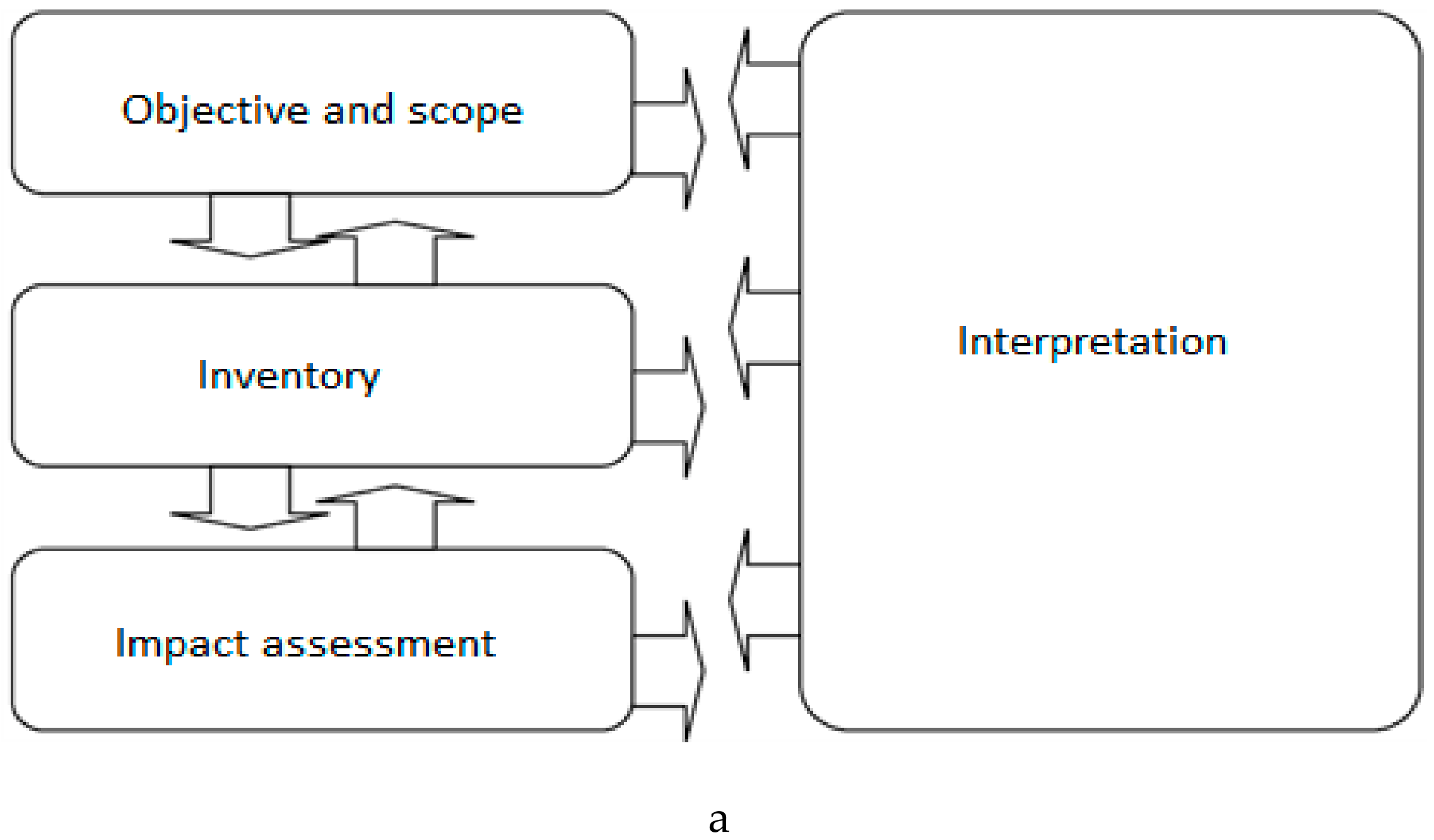
23], for example: (i) comparison of two entire systems or part of their life cycle; (ii) comparison between different phases of the cycle life; (iii) comparison of two different versions of the same system; and (iv) comparison of a system with a reference. The method also makes it possible to quantify an environmental impact on the complete life cycle of a product or only on one stage of the cycle without necessarily making a comparison. Thus, it is a tool that can not only serve as a decision aid, but also allows targeting of the phases of the life cycle of a product, which would need to be reworked with attention paid to the environment. The normative framework of the LCA [
20,
21] defines four different steps to follow: (1) the definition of the objective of the study; (2) the “Life Cycle Inventory” (LCI); (3) the “Life Cycle Impact Assessment” (LCIA); and (4) the interpretation of results—all these phases are organized independently and iteratively.
Specific standards were established for the LCA of the building sector by the European Committee for Standardization (CEN) in 2011: EN 15978 [
26] and EN 15643-2 [
27]. These standards are increasingly used to define and/or reduce the impacts of buildings on the environment. It is currently the only scientifically sound approach to carry out an environmental assessment at the building scale. It allows a quantitative study of the construction over their entire life cycle. However, its use at the urban or neighborhood scale is recent [
28,
29]. Despite the novelty of the LCA application at the neighborhood level, it is considered the most reliable method. It is a challenge and a fascinating research topic to test the application of the LCA method to an eco-neighborhood, especially since no other study to our knowledge has focused on the comparison of so many parameters and environmental indicators at the community level. Note also that many sustainable building certification schemes are based on the LCAs of the building materials [
30], such as BREEAM, DGNB and Valid in Belgium.
2.1. Building Scale
Several studies in different countries studied LCA at the building level.
In 2011, Rossi et al. [
25] compared the LCA of the same building located in three cities distributed in three different European countries and climates: Brussels (Belgium), Coimbra (Portugal) and Luleå (Sweden). A difference of less than 17.4% was obtained on comparing the operational energy and carbon. Stephan et al. [
31] analyzed the life cycle energy use in a passive building in Belgium and, then, carried out a comparison with other building types. The results showed that new techniques of construction had to be applied for improving the house energy efficiency. The passive house embodied energy accounts for 55% of the total energy on the 100-year life cycle. Cabeza et al. [
32] gave a review of the life cycle assessment (LCA), life cycle energy analysis (LCEA) and life cycle cost analysis (LCCA) in numerous kinds of buildings, located in different countries with varied climates. The results showed that few of the LCA and LCEA studies were carried out in traditional buildings. In their research, Kellenberger and Althaus [
33] carried out the LAC of many house components (roof, wall, etc.), with the purpose of evaluating the performance of the materials. The transportation of the building materials and other parameters were also studied. For deepening the knowledge of the environmental characteristics of the building materials and energy, Bribián et al. [
34] applied three environmental impact categories for comparing the most used material in the new designs. The results showed that the impact of a material can be significantly reduced by applying the new methods of eco-innovation. Vilches et al. [
35] showed that a majority of the LCA was based on energy demand compared at every stage of the life cycle. This research focused on the environmental impact of buildings system retrieval. A strong review on the life cycle energy analyses of buildings from 73 cases, applied in 13 countries and taking into consideration office and residential buildings, was shown by Ramesh et al. [
36]. Rashid and Yusoff [
37] assessed the phase and material that significantly affected the environment. In the research carried out by Chau and Leung [
38], the results showed that the use of different functional units did not allow easy comparison of the studies found in the literature.
2.2. Neighborhood Scale
We will now broaden the field of study and move to the neighborhood scale as a whole. Now that much progress has been made on the energy consumption of new buildings, other issues emerge [
39]. We emphasized the importance of focusing on phases other than occupation, whose relative impacts increase with a decrease in consumption [
40]. It is also necessary to tackle the thermal renovation in a more serious way. Beyond the building scale, the concepts of a zero-carbon city, a city without CO
2 or a post-carbon city are emerging around the world. Cities are now welcoming 50% of humanity. However, energy is not the only environmental problem. Cities are aware of the need to preserve biodiversity and green spaces [
41]. To achieve these different objectives, new tools and methods are needed, to be able to measure, at an urban scale, the consequences of architectural and urban choices on the environment [
41]. Many methodologies exist to quantify the environmental impacts at the city scale, but according to Anderson et al. [
42], LCA is again the dominant method at the urban scale. Indeed, after the study of the different existing methods, Loiseau et al. [
43] showed that LCA provides an appropriate framework and is the only method to avoid transferring environmental loads from one phase of the life cycle to another, from one environmental impact to another, or from one territory to another.
There is currently a need at the neighborhood level to integrate reflections on bioclimatic design, shared facilities, urban density or mobility issues, in order to achieve better environmental performance. Olivier-Solà et al. [
44] explained that it is highly likely that the environmental and energy issues we are currently dealing with at the building level will soon be transferred to the urban scale. Thus, neighborhood-level LCA is starting to get into practice. Some works and publications concerning this method have been written but they remain rare and heterogeneous [
45]. Some studies carried out by Ecole des Mines ParisTech within the energy and process center aim to scientifically develop the LCA method at the neighborhood level. The goal is even more ambitious because this work aims to make the method a tool for decision support, from the design phase [
41].
2.3. Goal
We want to study various parameters that impact the environmental balance of a neighborhood. We considered several environmental indicators that we detailed. We wished to identify the most important parameters that have the greatest impact on the environmental quality of a neighborhood. This may include, for example, orientation, the presence or absence of permeable soils, renewable energy sources or integration with public transit systems. Even if the general influence of some of these parameters was known, we wished to quantify precisely the environmental impacts and compare their importance with that of the other studied parameters. For this, we conducted the environmental analysis of a neighborhood and we varied the different design parameters to quantify their impacts. Thus, we were able to provide recommendations regarding certain design choices and their potential environmental impacts.
3. Methodology
This study is constituted of many important sections, such as (a) the survey; (b) modeling; (c) application of new scenarios; and (d) analysis.
3.1. Location
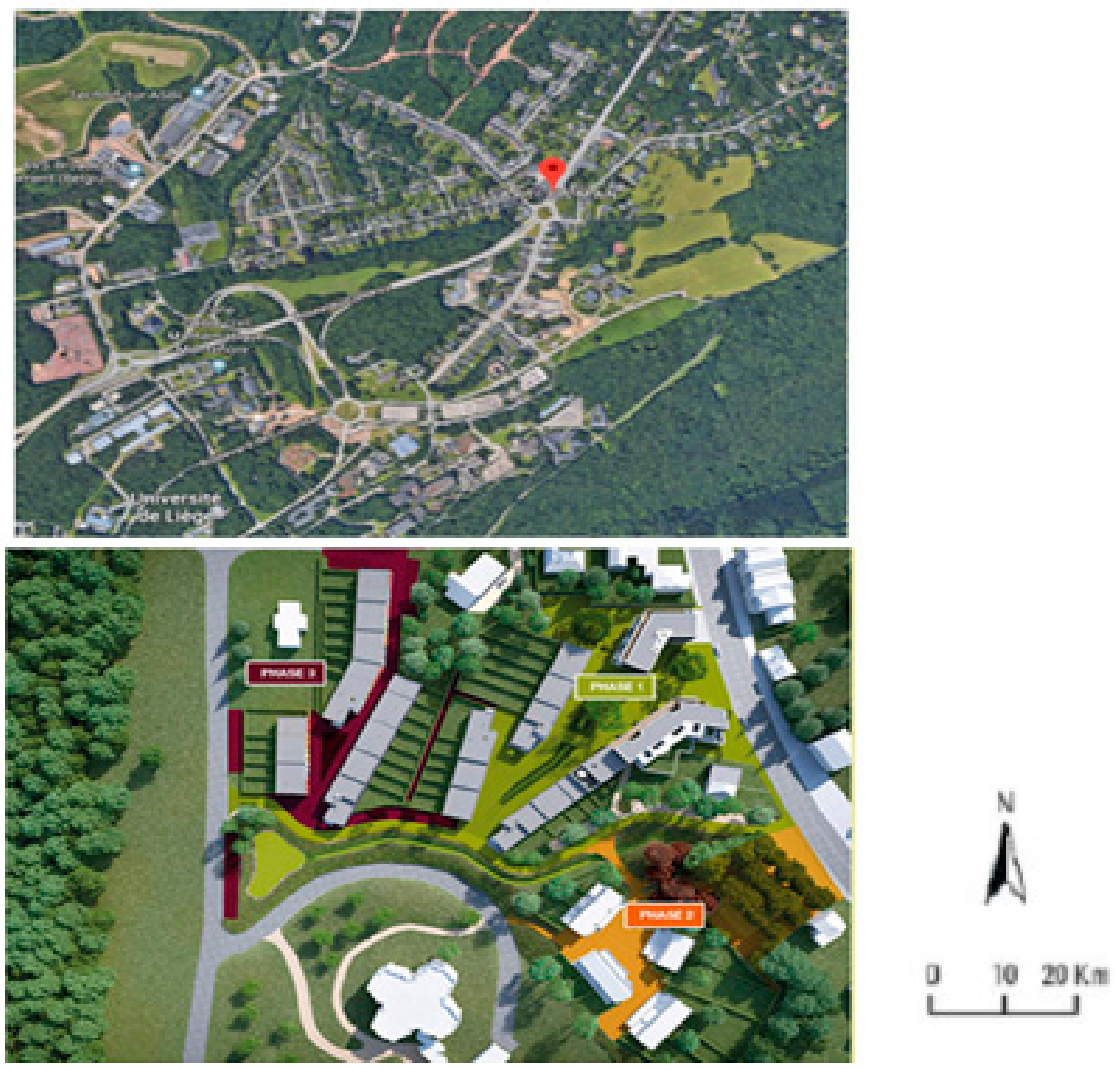
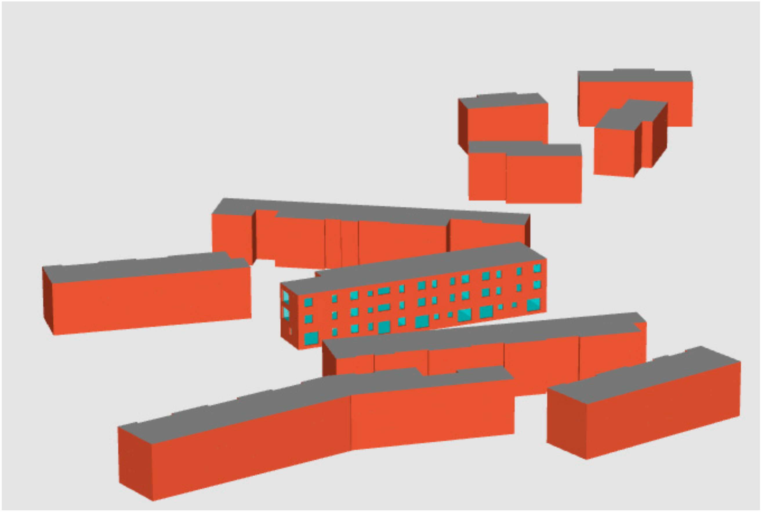
This study was carried out in a neighborhood located in Liege city in Belgium. This city is dominated by a continental climate in a temperate zone. During the year, we can note four seasons: winter, autumn, summer and spring. The neighborhood evaluated in this study is located nearby the University of Liege. This site is home to an extension of Liege University, and heavily dominated by green space, which is shown in
Figure 1. Several categories of buildings are found in this new neighborhood. Notably, there are apartments with two, three and even four facades. Most of these surfaces were developed for social housing.
Figure 2 and
Figure 3 show the location of this neighborhood.
3.2. Structure Analysis
In this city, several residences were considerate with respect to the energy demand suggested by international standards [
46,
47]. A total of 50% of the studied residences are semi-detached. This eco-neighborhood was built on a 3.51 ha plot. It has 17,000 m
2 of totally green space, and a total of 219 people in the residences. The life cycle assessment of the neighborhood is fixed at 80 years in the case of this study. We have taken some environmental data from the ECOINVENT database.
3.3. Simulation Tool
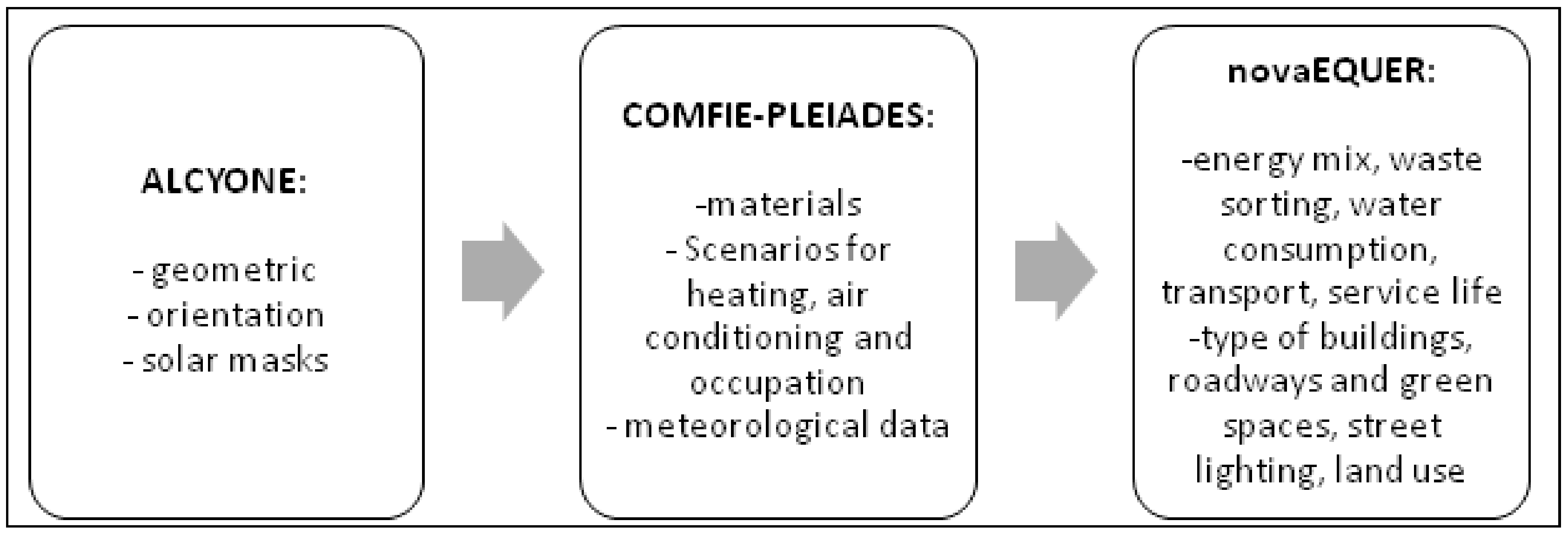
In this study, we used Pleiades software, version (4.19). It is divided into six modules: Library, Modeler, BIM, Editor, Results and LCA. Indeed, these tools were applied in several publications [
48,
49,
50,
51,
52,
53,
54,
55,
56]. The analysis chain was as shown in
Figure 3. Other different details regarding these simulation tools are also given in [
57,
58,
59,
60].
Under the base of the modeler tool of this software, it is easy to model all the buildings with their main characteristics. It is also possible to make the first simulations. All the results are automatically saved in the “result module”, which will be requested to evaluate the ACV of the neighborhood. The analysis of an LCA is not easy, because we must associate any constituent of the neighborhood in the software (buildings, roads, garden, water, people, climate, waste, energy mix, etc.). The environmental impact of all the main elements of the site is automatically added to form the global neighborhood.
3.4. Scenarios
Some methods applied in this research were found in [
54,
55,
56,
57,
58,
59,
60]. Globally, in this study, numerous scenarios were established, such as (1) building orientations; (2) water management; (3) mobility; (4) density; and (5) photovoltaic solar installation. It was very important to know the impacts of all these scenarios for improving the future planning of the new neighborhoods.
3.5. Modeling
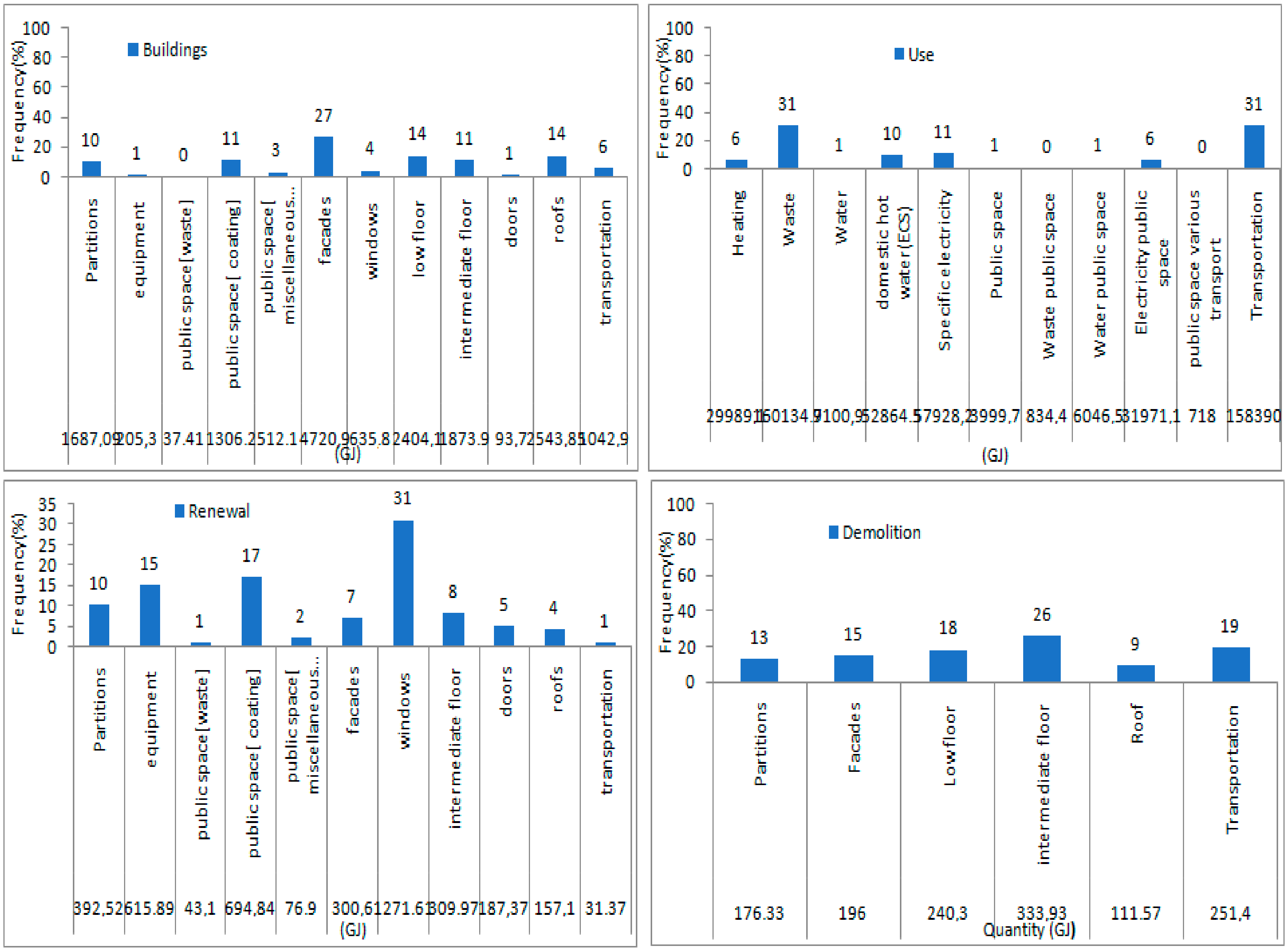
We began the modeling of our study area by studying the project’s characteristics data and the graphic modeling of the buildings on the site. A note was made of the geometrical parameters attributed to each of the walls of the buildings and their thermal properties, and the zoning and scenarios of use were also defined. Once all the parameters were defined, the dynamic thermal simulation calculations were started. All the characteristics of the buildings are described in
Table 1.
It was necessary to model some elements of our buildings, such as the walls, joinery, surface conditions and thermal bridges. With regard to the walls, we not only reveal the materials and elements of construction, their thickness, and their characteristics, but also the possible thermal bridges. At this stage, we have modeled the actual walls of the project with their precise characteristics. It is also necessary to obtain information on the surface state of the different walls, in order to manage their behavior with respect to radiation.
Table 2 and
Table 3 show the characteristics of the heat transmissions of the frame and glazing, as well as the thermal bridges.
The hourly temperature data, global and diffuse horizontal radiation, wind speeds, relative humidity, atmospheric pressure and precipitation of the studied sites, over the last forty years, were downloaded from American satellites by the Meteonorm software, and subsequently converted so as to implement them in the Pleiades software. We have modeled the walls, floors, slabs, roofs, openings and solar masks (
Figure 4). The geometries of the buildings and the actual openings have been scrupulously valued. The significance of modeling the neighborhood in three dimensions is that we now take into account the orientation and the solar masks that different buildings make on each other. In this manner, we will be able to study the impact of a change in the orientation of the mass plan or the increase in height of certain buildings.
3.6. Other Input Data
Several important results were obtained after simulation, such as (i) the detailed characteristics of all the simulated residences; and (ii) the different needs related to the consumption of water and energy. The lifespan of the different building materials was set at 80 years, such as those of the buildings.
There were different impacts resulting from the renovation phase. This different energy data were analyzed under the reference of the Belgian energy mix integrated in the software. According to the report of the International Panel of Climate Change in 2016, the Belgian energy mix is set at 4% coal, 27% natural gas, 17% renewable and 52% nuclear. It was important to notice that the consumption related to heating and domestic hot water (DHW) were calculated using the most recent data.
The supply system was a natural gas condensing boiler, having a 92% lower heating value (PCI) efficiency. The water consumption was estimated at 100 L/occupant/day. In the case of waste disposal, the new waste sorting policy was applied for this purpose (less waste.wallonie.be), which was set at 90% for glass waste and 75% for the paper and cardboard. This percentage of waste was applied as recycled, and not buried. With regard to the different Belgian statistics, it is found that 40% of the 1500 g of daily household waste per occupant are directly sent for incineration with an estimated yield of 85%, with the distance between the site and the landfill being 10 km, 100 km to the incineration plant and 50 km to the recycling site.
3.7. Orientation Scenario
We studied the different orientation effects of buildings at the neighborhood level. Initially, all the buildings were installed so as to more easily orient the different facades towards the south and the north. We have called this “scenario o”. Subsequently, we tried this test on several other orientations by guiding the mass plane to successive rotations of 45°, 90° and even 180°. Subsequently, we calculated the standard deviation of all the buildings studied affected by each of its orientations.
We chose the most unfavorable orientation to perform the LCA analysis of the neighborhood. Subsequently, we rigorously compared the different results of the new LCA in the neighborhood with that of the central neighborhood in order to evaluate the real effects of orientation on the LCA of a neighborhood.
3.8. Water-Use Scenario
The main objective of this new scenario is to collect all the rainwater and the discharged directly into a sanitary sewer network. If it were possible by pipeline to recover more than 95% of the rainwater in the different valleys, ditches, and cisterns, then it would be totally useless to evaluate the permeability of the different types of flooring. It is thus paramount to focus on two scenarios: one is based on the different rainwater collection systems and the other one is oriented towards the permeability of soils.
3.8.1. Rainwater Scenario
In the specific case of this scenario, we modeled all the rainwater tanks. In summary, rainwater was used to clean the interior and exterior of buildings, cleaning instruments, etc. In addition, reclaimed rainwater was fed from a separate network of reservoirs, ditches, valleys and water bodies. Garden water was collected by several ditches and turned towards the water. Rainwater from the roof was directly poured into the tanks. We assumed that all the rainwater from this place of study was controlled by a separate network.
3.8.2. Permeable Floors Analysis
In this scenario, we implemented more permeable floor coverings than in the basic option. In this manner, aisles, squares and car parks are constructed with unrepaired concrete pavements and concrete–grass slabs. Thus, the total impermeability of the site goes from 66% in the initial state to 58% once the permeable coatings are implemented. This small difference between the average permeability of the two scenarios is explained by the high proportion of green spaces in our neighborhood that do not see the modified permeability between the two scenarios. The large proportion of green areas of the site explains its relatively high permeability from the initial state. In this scenario, we consider that no other rainwater harvesting system be implemented. All of the water does not infiltrate directly into the soil; it is sent to the wastewater network.
3.9. Urban Mobility Impact Analysis
Let us now look at the impact of mobility on the neighborhood’s environmental record.
In our basic scenario we considered a significant use of the car for daily commuting. We will compare this scenario with a second one, where the site is considered urban, perfectly integrated with public transport networks and at a short distance from the shops of primary needs. Let us recapitulate the mobility hypotheses: (i) Initial scenario: 80% of the occupants commute daily; the 20 km distance from home to work is carried out daily by car; and the 5 km distance from home to the shops is done weekly by car. (ii) “Urban Site” scenario: 100% of the occupants make the trip, daily; the 2.5 km distance from home to work is done daily by bus; the 300 m distance from home to the shops is carried out weekly by bike or on foot.
3.10. Urban Density Impact Analysis
The purpose of these scenarios is to analyze the different effects of density on the life cycle of a neighborhood.
3.10.1. Vertical Scenario
We introduce another floor to each building. The configuration of the neighborhood remains the same. Overall, we are increasing the number of occupants as well as the construction area of our new neighborhood. The new district will have 100 more inhabitants than the old district.
3.10.2. Horizontal Scenario
The objective is to assess the impact of horizontal densification. For this, we decided to add some residential buildings on the used area (see
Figure 5). In total, four buildings were added. The total population is identical as in the reference scenario, which allowed us to keep the same configuration as that of the vertical density scenario. To achieve this goal, we had to occupy a small part of the public parking space. All the buildings added had the same characteristics as those existing; this in order to better compare these two methods and choose the best.
3.11. Urban Renewable Energies Use Impact
In the initial scenario, all the electricity used came from the Belgian electricity grid and the production impacts were taken into account. In this new configuration, we will have a photovoltaic system on all the roofs on the site, and we consider having a panel area equivalent to two-thirds of the roof area of each building. It must be noted that our homes use electricity only for light and to power household appliances. The installed installation will consist of mono crystalline photovoltaic solar panels. The sensors will be placed using a support on the roof terrace. They will be oriented south and inclined at 35°, the optimal inclination in Belgium. We then performed the thermal simulation of each building and completed the final LCA of the neighborhood.
4. Results
In this study, we obtained a heating requirement of 15.4 kWh/m²·year. The main requirement for meeting passive standards is to have a heating requirement of less than 15 kWh/m²·year. We notice that some buildings do not respect the passive standard. This may be due to their wrong orientation. The average results of the LCA under building scales are shown in
Table 4. These results showed that in the studied buildings, after 80 years, the average greenhouse gas was expected to be 2586.1 tCO
2 eq, while the cumulative energy demand would be 73,935.2 GJ.
The radioactive waste would increase to 76.5 dm
3. The waste water was from 58.593 m
3 /inhabitant per year. According to the research of Marique and Reiter [
24], heating energy was estimated to be between 190 and 200 kW h/m², in the case of the conventional neighborhood. In this case, the heating energy is around 16 kW h/m
2 as requested by several international standards. Moreover, according to Lotteau et al. [
29], the greenhouse gas is between 11 and 124 kgCO
2/m
2; in this research, it is around 35 kgCO
2/m
2. This means that the results found in this research are in the range given in the literature.
The average odor concentration was 32.162 Mm
3air/inhabitant per year.
Table 5 shows some simulation results of the LCA on the neighborhood scale. It was seen that the total greenhouse gas was expected to be 21,733.64 tCO
2 eq after 100 years, whereas the total cumulative energy demand was 532,385.49 GJ. The health damage was 22.29 DALYS (disability-adjusted life years), and the potential for degradation related to land use obtained was 28,630.00 m
2/year.
DALYs are the sum of the YLDs and YLLs, per disease category or outcome, and per age and sex class:
where YLD (the morbidity component of the DALYs) = number of cases * disease duration * disability weight; YLL (the mortality component of the DALYs) = number of deaths * life expectancy at age of death.
It was interesting to notice that the total eutrophication assessed was 42,794.03 kg PO
4 eq. The analysis of the most important sources of impact (greenhouse gas and cumulative energy demand) and their distributions according to the different stages of the life cycle is given in
Figure 6 and
Figure 7. In
Figure 6, we notice the strong predominance of the occupation phase, which concentrates on 93% greenhouse gas production. In this phase, mobility is strongly in the majority with 46% emissions. Heating and domestic hot water accounts for 24% of emissions, while waste treatment accounts for 15% of the emissions during the use phase. Only 1% of greenhouse gas comes from a “public space”. It is interesting to note that emissions from the household waste management are equivalent to those from the production of hot sanitary water (15% of the use phase emissions), whereas the emissions from heating accounted for only two-thirds of the emissions, from the production of hot sanitary water.
Emissions due to the mobility of the inhabitants accounted for almost half of the emissions from the use phase. These characteristics were perhaps due to the fact that the high thermal performance of our buildings greatly reduced their heating consumption.
Figure 7 showed the impact of cumulative energy demand defined in [
61] .As in the previous
Figure 6, it was seen in this figure that the use phase was predominant (96% of the cumulative total energy demand). This could be due to the accounting for mobility and waste management. The cumulative demand for energy due to waste management was almost identical to that due to the mobility of residents and was equivalent to almost one-third of the demand of the occupancy phase. In addition, this was because the cumulative energy demand from transportation and waste management during the use phase was 60% of the total cumulative energy demand of the neighborhood, over its entire life cycle. Meanwhile, the cumulative energy demand due to “the heating and domestic hot water” was only half of that required for the transport of inhabitants or the management of household waste. These different results show a very strong participation of the mobility component and the household waste management component in the LCA at the neighborhood level.
4.1. Orientation Impact Assessment
This section studied the orientation impact assessment of the LCA outcomes at the neighborhood level.
Figure 8 showed the comparison of the environmental impacts of the established scenarios to “0° orientation” and “90° orientation”, in percentage. We noted that once all the neighborhood-level impacts were accounted for, the influence of the orientation became minimal. Indeed, it was mainly on the greenhouse effect, on the cumulative demand of energy, and on the depletion of the abiotic resources that the orientation had an important effect. This was due to the change in energy consumption due to heating. However, we observed only a relative increase of less than 1% of these impacts. Moreover, this evolution only affected the phase of use. On the other hand, we observed a 1% increase in greenhouse gas emissions, as well as the depletion of abiotic resources and cumulative energy demand during the use phase in the case of a rotation to 90°. This is could be due to the increase in gas consumption caused by the increase in heating needs.
Comparing the scores of the environmental indicators only for the heating items during the use phase, as also for both orientations, we notice an 11% increase in the greenhouse effect, as well as a cumulative energy demand and depletion of abiotic resources for the 90° orientation. Thus, the orientation has an impact on heating consumption and on environmental indicators relating only to these [
62,
63,
64,
65]. However, at the neighborhood level, this orientation has little impact on the overall results of the LCA. However, even if the orientation has little influence on the LCA results at the neighborhood level, at the building level it can be decisive, especially for obtaining the passive label.
The different quantities of environmental impacts are shown in the
Table 6.
4.2. Water Management Impact Assessment
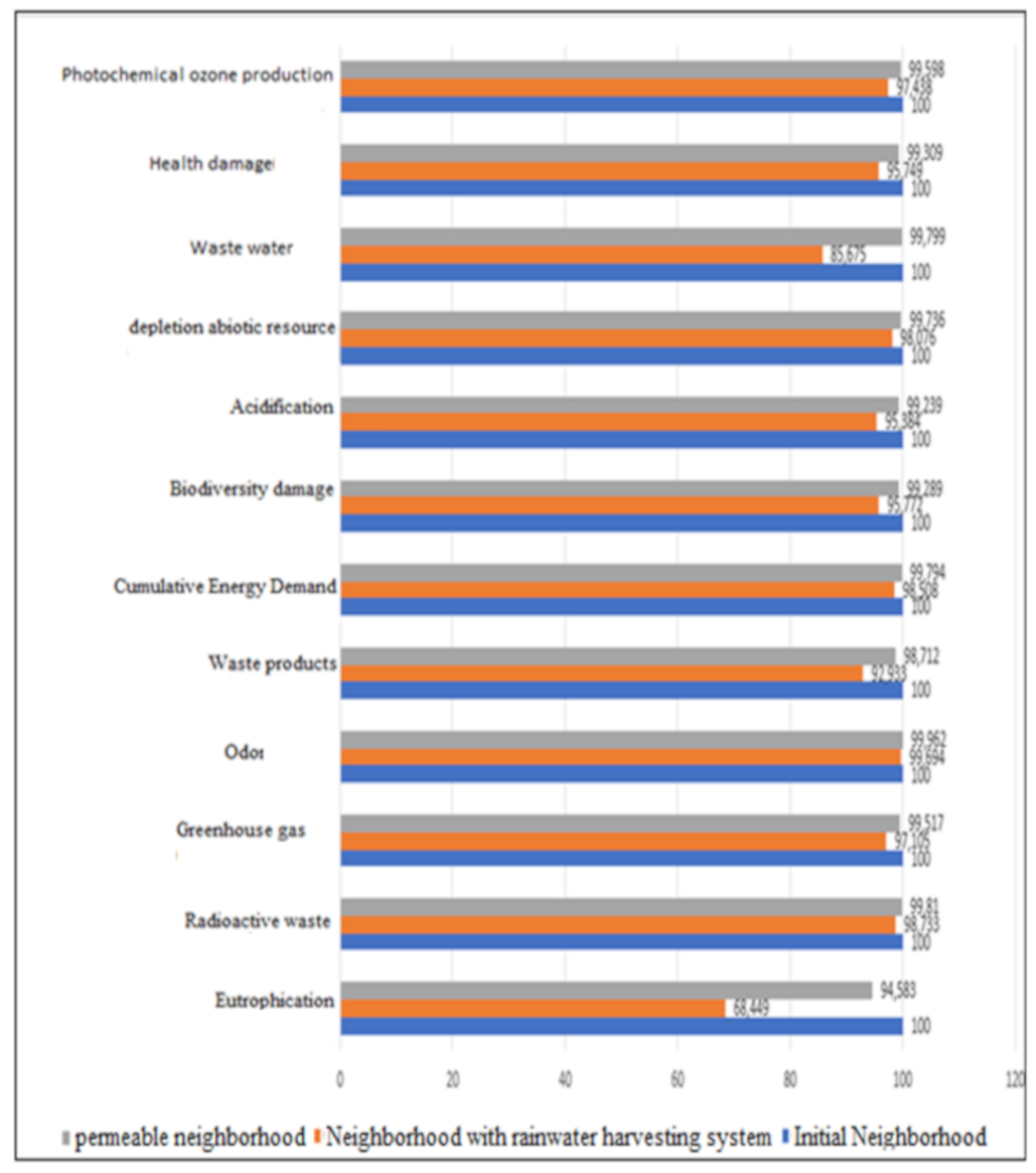
In
Figure 9a, we note that setting up rainwater harvesting systems has a strong impact on certain environmental indicators. Indeed, collecting all the rainwater can reduce eutrophication by 32%. This significant decrease is due to the fact that the runoff water is entirely recovered on the site by the valleys and infiltration basins. Thus, the nutrients are not strained, but retained on the site. On the other hand, it was noticed that drinking water consumption is also strongly impacted. Indeed, with a well-sized tank, it is possible to use only rainwater to feed the washing machines and flushes with water. This will save drinking water up to 6000 L per person per year, which implies a 14% reduction in water consumption of the neighborhood on a scale of its total life cycle—a 7% decrease in waste produced over the entire life cycle of the neighborhood. Indeed, on the use phase, 15% less waste is produced. This is the runoff water that is no longer directed to the treatment plants, and therefore no longer needs to be treated. Moreover, we have observed a decrease of about 4% in damage to biodiversity, damage to health and acidification.
The analysis in
Figure 9b shows that the impact of soil permeability on the total LCA of the neighborhood is lower. In fact, the concerned indicators are still eutrophication and waste production. In this case, the use of permeable soils reduces the impact of eutrophication by 5% and the production of waste by 1% over the entire life cycle of the neighborhood. In fact, the amount of water that infiltrates into the ground, thanks to the permeable pavements, is less than the quantity that can be recovered by the recovery systems presented in the previous scenario.
Figure 10 shows the comparison of the three scenarios (initial scenario, and with and without permeable floor coverings). The analysis of this figure shows that it is more efficient to install recovery systems like cisterns, valleys or infiltration basins at the neighborhood level. However, implementing permeable floor coverings on areas that cannot benefit from recovery systems will have a positive impact on the amount of wastewater to be treated and on eutrophication.
4.3. Mobility Flow Impact Assessment
This section analyzed the impact of mobility on the neighborhood’s environmental record.
Figure 11 shows an analysis of the environmental impact on the mobility scenarios. It is seen that all environmental impact indicators are reduced from 6% to 50%. Seven indicators out of 12 are reduced by more than 20%. Thus, it was concluded that mobility has a significant impact on the neighborhood’s environmental record.
“Photochemical ozone production” is reduced by more than 50% over the entire life cycle of the neighborhood. In fact, the combustion of fuels is the main source of nitrogen oxide production, which transforms into ozone under the effect of sunlight [
64]. In our urban site scenario, 54% of photochemical ozone production in the use phase is avoided, by reducing the use of automobiles. Indeed, 95% of transport-related ozone production during the operational phase is avoided in this scenario. Another photochemical ozone production station is waste management. The previous figure (
Figure 11) shows the same observation with the “greenhouse gases”. Indeed, a decrease of 40% of the emissions is observed on the total life cycle of the neighborhood, thanks to a decrease of 93% transport emissions during the use phase. On the other hand, it is interesting to note that “acidification” has also been strongly impacted by the suppression of automobile use. We have observed a 35% decrease in this impact indicator over the entire life cycle of the neighborhood. It is the same for “depletion of abiotic resources” and “damage to health”, which saw their score reduced by 34% and 32%, respectively. Indeed, much less fuel and fossil resources are consumed and the pollution responsible for many health problems is also greatly reduced.
Decreasing the use of cars can create huge savings in energy. Public transport uses the energy contained in fuels in a more efficient and rational manner. Thus, the cumulative energy demand is reduced by 28%. It is also shown that there has been a 23% decrease in damage to biodiversity, 17% in eutrophication, 15% in radioactive waste, 13% in odors and 6% in waste produced.
Detailed responses on the urban mobility are showed in
Table 8.
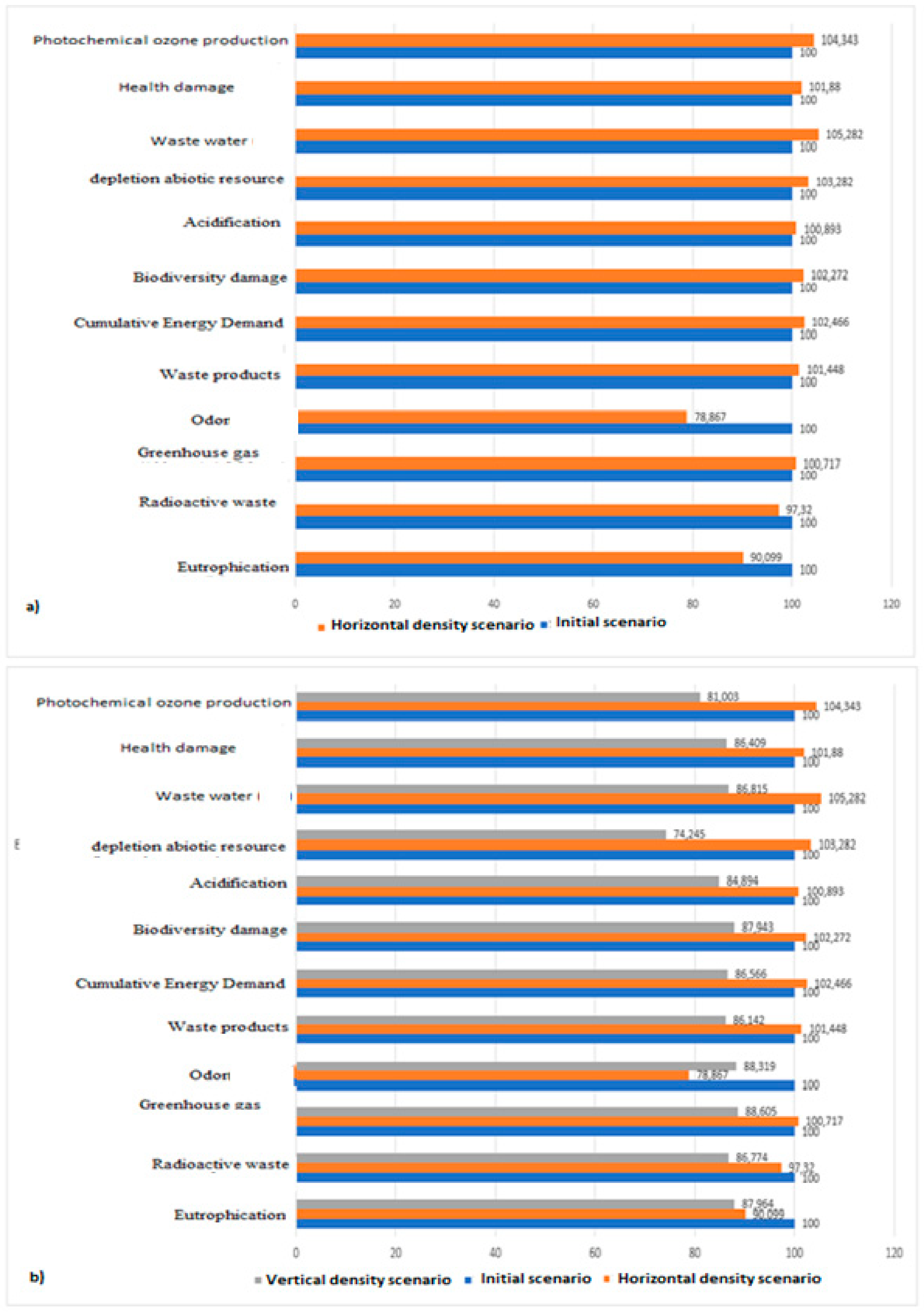
4.4. Density Impact Assessment
Table 9 estimates the heating requirements of the various buildings in the study area.
Analysis of this data showed that the heating requirements with an additional floor dropped slightly. We thought that the additional shading created should act as solar masks, which would reduce solar gain and increase heating needs. However, it seemed that the increase in compactness caused by the rise of the buildings was more impacting.
Figure 12 shows the comparative diagram of the environmental impacts of the scenarios.
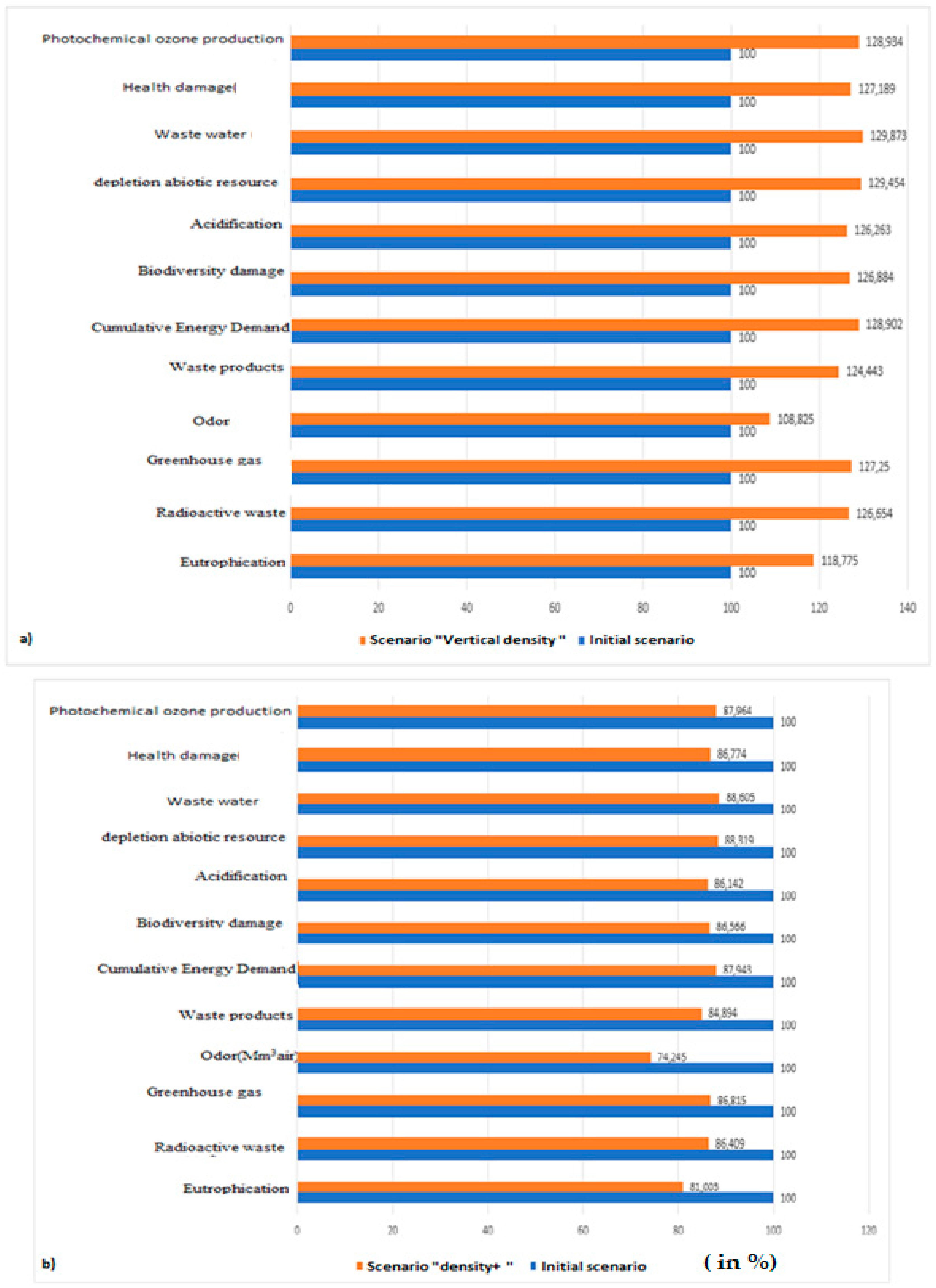
In
Figure 12a, the results are expressed on the basis of a functional unit encompassing the entire neighborhood. This is because the indicator scores had all increased in fairly similar proportions, from about 25% to 30%. Indeed, the share of the indicators related to the buildings was modified, but not that related to the district, which remained unchanged. This functional unit did not allow us to draw any interesting conclusions. This is why we are going to translate the results of the study into the “Occupant” functional unit, to be able to compare per capita impacts in both configurations.
As shown in
Figure 12b, if we compare the environmental indicators by reporting them to the number of inhabitants, we notice that the high-rise one-story has a better environmental performance. The odor indicator is reduced by 26% and eutrophication by 19%. The other ten indicators are reduced between 11% and 15%. Indeed, even the site welcomes more occupants and the consumption by these added to the initial consumption, all impacts from the site itself and public spaces remain unchanged. Thus, the built surface is more profitable.
In the case of an increase in density built by adding buildings to the site (
Figure 13a), the results were not as favorable as in the previous case. In fact, apart from odors, radioactive waste and eutrophication, the scores of which decreased by 21%, 3% and 10%, respectively, the other indicators had increased. They all earned between 1% and 5%. Indeed, we did not benefit here from a gain in compactness and we did not pool the networks. In addition, the construction of new buildings was greener in materials and energy than the rise of a floor. The analysis of
Figure 13b showed that densifying the neighborhood vertically was more remarkable environmentally. The impact on the total LCA of the district was much more pronounced than during horizontal densification, for which the assessment was mixed.
Some results are showed on the
Table 10.
4.5. Impact of Renewable Energy Uses
Taking into account the dynamic thermal simulation, the consumption and electricity production were calculated. For all buildings, production exceeded consumption throughout the year, except for the months of December and January, where the installation covered 45% and 75% of the consumption, respectively. In fact, the buildings consumed, on an average, 12 kWh/m² of electricity per year. These results were consistent with the Belgian averages for dwellings that did not heat up with electricity. Photovoltaic panels produced an average of 26 kWh/m² over the year. Thus, except for the months of January and December, no electrical energy was drawn from the Belgian network. The effects on the LCA of the neighborhood are presented in
Figure 14.
Of all the configurations studied, the one comprising the addition of photovoltaic panels is the one that produces the most heterogeneous results on the neighborhood’s LCA. Indeed, some indicators are greatly reduced, while others see their score increase considerably.
The most affected impact is the production of radioactive waste. Over the entire life cycle, the production of radioactive waste is reduced by 102%. Indeed, even if this production of waste increases during the construction (9%) and renovation (1893%) phases, because of the impact of the manufacture of panels, the use phase makes up for this delay. The enormous increase in the usage phase score is explained by the fact that the panels are changed every 20 years and that in the previous scenario, the production of radioactive waste of this phase was insignificant. That being said, the production of radioactive waste during the use phase decreases by 127%. This is explained by the fact that production is higher than consumption. As a result, not only is the construction and maintenance of the system offset, but the production of radioactive waste from the use phase is also eliminated. Moreover, it allows other homes to benefit from the clean energy produced. Thus, our neighborhood reduces the production of radioactive waste from other neighborhoods, which gives a negative score for this indicator.
The second-most impacted indicator is the cumulative demand for energy. The total energy needed by the neighborhood to operate over its entire life cycle is reduced by 37%. Once again, the construction and renovation phases are negatively impacted. The construction phase saw its energy consumption increase by 75% and the renovation phase by 978%, due to the manufacture of the panels. However, the occupation phase saw its demand decrease by 47%.
The depletion of abiotic resources and the greenhouse effect also decreased by 14% and 12%, respectively, over the entire life cycle. The evolution of the indicators once again followed the same pattern: a significant increase in the construction and renovation phases. However, once again these increases are offset by a reduction in the environmental impact of the use phase, the most impactful phase of the life cycle. We observed a 25% drop in greenhouse gas emissions over this phase and a 26% decrease in the depletion of the abiotic resources.
Conversely, some indicators see their score increase. This is the case of the production of waste. The renovation phase saw its waste production increase by 742%. In fact, 4400 m
2 of the panel area had to be replaced thrice over the neighborhood’s life cycle and in addition included their initial installation. The 15% decrease in waste production during the use phase did not make up for this increase. As a result, the neighborhood’s total waste generation over its entire life cycle was up by 21% (
Figure 14). Some results are showed on the
Table 11.
Finally, paradoxically, the damage done to biodiversity is also increasing. It is again the manufacture and the replacement of the panels which is in question. The impact of the construction phase increases by 229% and that of the renovation phase by 849%. The 6% drop in impact during the use phase does not compensate for these losses. Thus, over the cycle, the damage to biodiversity increases by 18%.
4.6. Global Analysis of All the Scenarios
In order to classify the different scenarios and define the design parameters to take into account their priority, we calculated the sum of the variations, as a percentage of all the indicators compared to the initial scenario. We chose to apply no weighting but will remove the indicator “odors”, which distorts the results by its important variations.
Table 12 shows some obtained results.
It was noted by analyzing this table that mobility has an impact of 282% of the cumulative decrease on all indicators: vertical density (163%), renewable energies (138%), rainwater harvesting (76%), soil permeability (11%), orientation (4%) and horizontal density (−10%).
5. Discussion
Overall, it was seen in this study that the installation of photovoltaic panels has a mixed record. Indeed, the installation was heavily oversized. Several results found in this research are similar to those assessed by Lotteau et al. [
65,
66]. Indeed, those asserted by Lotteau et al. [
65] and the divergence of methodology among different researchers with regard to LCA prevented an easy comparison of results at the neighborhood level. However, in the known research, several aspects common to the LCA were studied, such as (i) the operational energy consumption analysis of buildings; (ii) the quantitative analysis of the construction materials; and (iii) the transport requirement analysis and so on. The process ranged from statistical data collection from neighborhoods to detailed simulations based on physical modelling. Mobility management was the most significant element. Indeed, it was the parameter that allowed a reduction in most of the impacts in terms of greenhouse effects, odors, damage to biodiversity and health, acidification, depletion of abiotic resources and photochemical ozone production. The day-to-day use of individual transportation by local residents has a huge impact on the neighborhood’s LCA. Eliminating the use of personal vehicles for the benefit of public transport makes it possible to limit the greenhouse effect four times more than to generate all the electricity of the district, thanks to the photovoltaic panels. Thus, mobility management must be one of the issues to be addressed as a matter of priority in any urban reflection. Designing a neighborhood that is sustainable and environmentally friendly, while being disconnected from public transport, is not always the ideal solution. In the past, Mohamad Monkiz et al. [
67] also found that mobility management was one of the most important aspects in the LCA study. The criterion of vertical density was also a fundamental element. Increasing the built density of the neighbourhood by elevation of the buildings was environmentally very beneficial. This made it possible to pool many flows, to increase the energy and environmental efficiency of the neighbourhood, and, thus, homogeneously minimize the different environmental impacts. These results were almost similar to those of André Stephan et al. [
16], who found that by replacing an area, part suburb, with apartment buildings, allowed to decrease the total energy consumption by 19.6%.
An eco-district must therefore have a certain density. One of the criteria for a sustainable neighbourhood covers this aspect and imposes a density of 30 to 40 dwellings per hectare [
68,
69]. It was found in this study that the implementation of renewable energy production systems showed a significant environmental balance, as was seen in several research results [
70]. This method was useful for limiting the production of radioactive waste and for the cumulative demand for energy. However, the manufacture of photovoltaic panel systems has a negative impact on the LCA in terms of damage to biodiversity and waste produced. Thus, their large-scale implementation does not necessarily seem to be a priority, at least not until their manufacturing and recycling processes are cleaner. On the other hand, integrating rainwater harvesting systems into the neighbourhood has been shown to have a strong impact on the results of an LCA, especially in terms of eutrophication and water use. Intelligent rainwater management should be a priority when designing a neighbourhood. Finally, soil permeability and orientation are parameters that can also improve the environmental record of a neighbourhood, but to a lesser extent. As for the choice of applying the concept of horizontal density to the neighbourhood, by adding more buildings, it can be counter-productive. In the studied neighbourhood, it is seen that the annual energy savings and avoided GHG emissions were less significant than those recorded in one neighbourhood of New York City (7.3 GJ and 0.4 metric tonnes). The main results of this research may be of interest to construction companies, public officials and decision makers for applying the environmental criteria to the planning process of new and existing neighborhoods.


