Article

Citrus Disease Image Generation and Classification Based on Improved FastGAN and EfficientNet-B5

1
College of Electronic Engineering (College of Artificial Intelligence), South China Agricultural University, Guangzhou 510642, China
2
Division of Citrus Machinery, China Agriculture Research System, Guangzhou 510642, China
3
Guangdong Engineering Research Center for Monitoring Agricultural Information, Guangzhou 510642, China
*
Author to whom correspondence should be addressed.
Agronomy 2023, 13(4), 988; https://doi.org/10.3390/agronomy13040988
Submission received: 1 March 2023 / Revised: 23 March 2023 / Accepted: 24 March 2023 / Published: 27 March 2023

Abstract

:
The rapid and accurate identification of citrus leaf diseases is crucial for the sustainable development of the citrus industry. Because citrus leaf disease samples are small, unevenly distributed, and difficult to collect, we redesigned the generator structure of FastGAN and added small batch standard deviations to the discriminator to produce an enhanced model called FastGAN2, which was used for generating citrus disease and nutritional deficiency (zinc and magnesium deficiency) images. The performance of the existing model degrades significantly when the training and test data exhibit large differences in appearance or originate from different regions. To solve this problem, we propose an EfficientNet-B5 network incorporating adaptive angular margin (Arcface) loss with the adversarial weight perturbation mechanism, and we call it EfficientNet-B5-pro. The FastGAN2 network can be trained using only 50 images. The Fréchet Inception Distance (FID) and Kernel Inception Distance (KID) are improved by 31.8% and 59.86%, respectively, compared to the original FastGAN network; 8000 images were generated using the FastGAN2 network (2000 black star disease, 2000 canker disease, 2000 healthy, 2000 deficiency). Only images generated by the FastGAN2 network were used as the training set to train the ten classification networks. Real images, which were not used to train the FastGAN2 network, were used as the test set. The average accuracy rates of the ten classification networks exceeded 93%. The accuracy, precision, recall, and F1 scores achieved by EfficientNet-B5-pro were 97.04%, 97.32%, 96.96%, and 97.09%, respectively, and they were 2.26%, 1.19%, 1.98%, and 1.86% higher than those of EfficientNet-B5, respectively. The classification network model can be successfully trained using only the images generated by FastGAN2, and EfficientNet-B5-pro has good generalization and robustness. The method used in this study can be an effective tool for citrus disease and nutritional deficiency image classification using a small number of samples.

1. Introduction

Citrus is one of the most popular fruits in the world. However, for a long time, diseases have seriously threatened the growth of citrus. They affect the yield and quality of citrus crops and have a significant impact on the citrus industry. In severe cases, the diseases can lead to the death of an entire citrus patch. Therefore, improving citrus disease prevention technology to effectively prevent the appearance of diseases and produce citrus fruit trees with high yield and quality is crucial. The traditional identification of citrus pests and diseases relies on the naked eye, which takes a long time and requires certain professional knowledge. An intelligent, low-cost, and highly accurate method for citrus disease identification would be more practical [1] (see Abbreviations Section).
In recent years, deep learning technology has been widely used in the field of agriculture, such as in fruit classification and grading [2,3,4], automatic picking, and the diagnosis of diseases and pests [5,6,7,8], and the automatic diagnosis of plant diseases is one of the most active research areas in agriculture. Several deep learning-based techniques for automatic plant disease diagnosis have emerged, which can help farmers reduce the economic losses caused by pests and diseases in farming [9]. In crops, disease symptoms often appear on the leaves; therefore, crop diseases can be automatically detected by applying machine learning techniques to leaf images. For example, Zhang et al. [10] segmented diseased leaf images using K-means clustering and extracted shape and color features from the lesion information. They classified seven cucumber diseases using sparse representation with a presidential recognition rate of 85.7%. Liu et al. [11] proposed a WSRD-Net method for wheat stripe rust detection based on a convolutional neural network (CNN), which can obtain 60.8% average precision (AP) and 73.8% recall rate on a wheat stripe rust dataset. Zhong et al. [12] proposed a three regression, multi-label classification and focal loss function methods based on the DenseNet-121 deep convolutional network to identify apple leaf diseases with over 93% accuracy on 2464 images, including six apple leaf diseases.
Yao et al. [13] used an improved Xception network to classify brown spots and anthracnose of peach, eventually obtaining a 98.85% accuracy [14]. Janarthan et al. [15] proposed a lightweight, fast, and accurate deep metric learning-based architecture for detecting citrus diseases from sparse data to obtain 95.04% detection accuracy. Deep learning requires many datasets to support the model training. Otherwise, overfitting may occur [16]. The main obstacle to using machine learning in agriculture is the small dataset and the limited number of annotated samples. This becomes more evident when supervised machine learning algorithms that require labeled data are used. The collection of a large amount of plant-disease-related data may have the problem of an uneven distribution of samples. Some diseases may have a small number of samples, which is not enough to train a classification network. Although some public datasets are available, the size of the datasets and categories do not meet the requirements of all applications. Using simple data enhancement methods such as random inversion, deep random flip, increasing contrast, and adding noise [17] can suppress overfitting, but the sample data are still not sufficiently rich, and the image features are less differentiated from the original dataset. Goodfellow et al. [18] proposed a generative adversarial network (GAN) using generators and discriminators against each other. GAN is widely used in the field of computer vision, such as for image super-resolution reconstruction and image defogging [19,20], and can also be used as a data enhancement tool to expand datasets [21]. Using generated images introduces more variability, which can improve the training process of classification networks and increase accuracy.
Ma et al. [22] generated blood cell images using a DC-GAN network to increase data samples and eliminate data imbalance and missing data labels. Cap et al. [23] proposed a LeafGAN by improving CycleGAN using paired datasets to successfully transform healthy leaves into diseased leaves. Xiao et al. [24] successfully generated six types of citrus leaf images using TRL-GAN, an enhanced version of CycleGAN that removes the real scene background from the original images using Mask RCNN. They achieved a 97.45% accuracy on ResNeXt101 after expanding the original dataset using the generated images. However, expanding datasets with adversarial networks increases training time, mostly to several days, and generates low-quality images. The resolution of the generated images is often below 512 × 512, which cannot retain more details, and the expanded dataset has limited performance improvement for the classification network.
Karras et al. [25] proposed StyleGAN2 based on StyleGAN. The StyleGAN is a current high-performance, high-resolution image generation framework capable of generating very high-quality images on a wide range of datasets but still requires a large dataset as well as high computational resources and training time [26]. Liu et al. [27] proposed the FastGAN network, which can finish training a complete model in a dozen hours on a single RTX-2080 GPU, by improving StyleGAN2. However, when applied to plant disease sample generation, it produces checkerboard artifacts, loss of details, and insufficiently rich sample data. The performance of the classification model degrades significantly when the training and test data are very different in appearance or originate from different regions, for example, the light of the target in the training data is very strong while the light of the target in the test data is very dark, the image acquisition devices are different, the geographical locations where they were taken are different, and so on.
Mohanty et al. [28] used 54,306 healthy and diseased leaf images from the PlantVillage dataset to train a neural network model for the identification of 26 leaf species and obtained an accuracy of 99.3% after cross-validation evaluation. The performance of the model decreased to approximately 31% when tested with a set of plant images taken in the field because the training set of the model was taken in a laboratory environment, and its images had a uniform background. Ferentinos [29] also noted that when the model was trained on images taken in a laboratory environment and tested on images taken in a planting environment, the accuracy of the model decreased from 99.5% to approximately 33%. Therefore, changes in background and shooting conditions can have a serious impact on the performance of the model.
Because the background of the FastrGAN2-generated images is not as rich as that of the real captured images, the FastrGAN2-generated images and captured images can be regarded as coming from different regions. Because our experiments only used the FastrGAN2-generated images as the training set to train the model and the real captured images to test the performance of the model, this poses a classification network performance challenge and requires the classification network to have a high generalization capability.
Here, we propose the FastGAN2 network, which overcomes the checkerboard artifact problem of the FastGAN network, improves the quality of generated images, and enhances the diversity of the generated images for small datasets. We used the generated images only as the training set of the classification network and tested it using images taken but not used for training with the FastGAN2 network. Finally, we tested it on Densenet121, ResNet50, ShuffleNetv2 [30], Mlp-Mixer [31], MobileNetv3 [32], Vision Transformer, Swin Transformer, EfficientNet-B3, EfficientNet-B5 [33], and EfficientNet-B5-pro and achieved an average accuracy of 93.52%. To improve the generalization of the model, this paper proposes an EfficientNet-B5-pro network based on EfficientNet-B5 that uses the adaptive angular margin (Arcface) loss with adversarial weight perturbation (AWP) mechanism. It achieved the highest performance compared to ten classification networks. The main contributions of this study are as follows:
By redesigning the FastGAN network generator structure and adding small batch standard deviations to the discriminator to eliminate checkerboard artifacts, the im-proved FastGAN is more suitable for citrus disease and nutritional deficiency (zinc and magnesium deficiency) image generation. It can generate higher-quality and more realistic disease and nutritional deficiency images with higher diversity when trained on a small number of datasets.
The datasets of citrus melanose, citrus nutritional deficiency, and citrus canker leaves were expanded, and the generated images had the phenotypic characteristics of the real data. With a small dataset, a classification network with 97.04% accuracy was trained using only the generated images, which could successfully identify the four types of citrus leaves.
EfficientNet-B5-pro is proposed, which improves EfficientNet-B5 by using the AWP mechanism and Arcface loss. It has better robustness, better generalization ability, and higher accuracy compared to the unimproved EfficientNet-B5.

2. Materials and Methods

2.1. Dataset and Test Environment Setup
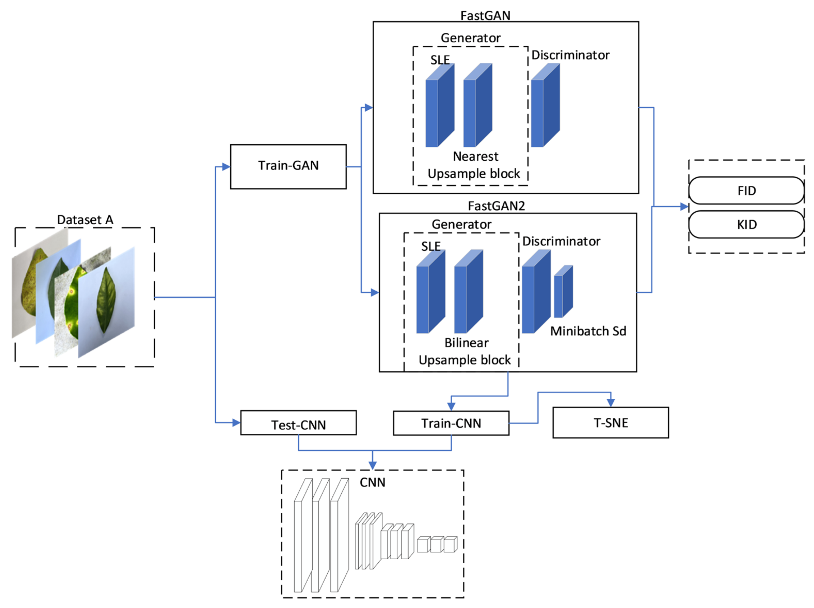
Nutritionally deficient citrus leaves and healthy citrus leaves used in this study were collected from the orchard of the eastern district of South China Agricultural University. Citrus canker leaves were collected on rainy days from the citrus orchard of Dingkeng village, Aotou Town, Conghua district, Guangzhou, China, and citrus melanose leaves were obtained from published data on the Kaggle competition [34]. The collection device was an iPhone 13 Pro Max, the shooting distance was 15–30 cm, the picture resolution was 3024 × 4032 pixels, the picture storage format was JPG, the picture dates were 18 and 25 May and 15 and 25 July 2022, and the shooting times were 10:00–12:00 and 14:00–17:00. The shooting scene was in natural light conditions. A total of 256 citrus canker leaves, 237 healthy citrus leaves, 224 nutritional deficiency citrus leaves, and 192 citrus melanose leaves were collected. Images are shown in Figure 1.
All collected images were used as the original dataset A. Fifty images of each of the four diseases in dataset A were randomly selected as the training set Train-GAN for the GAN network. The remaining images were used as the test set Test-CNN for the classification network. Using the trained FastGAN2 network, 2000 images were generated for each class of disease separately as the training set Train-CNN. The detailed numbers of different species of leaves can be found in Table 1.
In the training of the FastGAN2 network, the epoch number was set to 30,000, the batch size was set to 8, the input image size was 1024, the learning rate of the generator and discriminator was 0.0002, and the optimizer was Adaptive Moment Estimation (Adam). In the training of the classification network, the batch size was set to 16, the input image size was 256, the cosine annealing learning rate strategy was used [35], and AdamW was the optimizer [36]. The experiments were conducted on Ubuntu 20.04 with Python 3.8, PyTorch 1.10.0, and Cuda 11.3. The graphics card was RTX3090 with 24 GB of video memory, and the CPU was AMD EPYC 7543. The framework flowchart of generation and classification model are shown in Figure 2.

2.2. FastGAN Model

The FastGAN model was proposed by Liu et al. [27]. The authors improved StyleGAN2 by designing the SLE (skip-layer excitation) module, which shortens the training time of the original model from several days to a dozen hours. They also proposed a self-supervised discriminator that can train the network more stably with a small number of training samples and limited computational resources.
When synthesizing higher-resolution images, the G (Generator) must be deeper and have more convolutional layers to meet upsampling requirements. The more convolutional the layers, the longer the training time of the model. He et al. [37] designed the residual structure ResBlock, which uses cross-layer connections to enhance the gradient signal between the layers. However, this also increases computational costs. The idea of cross-layer connectivity has been reconstructed in the SLE module. This module implements the skip connection as the summation of elements between activations from different convolutional layers, which requires the same spatial dimension of activations. The module also eliminates the heavy computation of convolution by replacing addition with multiplication, as shown in Equation (1), to perform skip connections between different resolutions:
y = F x low   , W i x h i g h
In the formula, x and y are the input and output feature maps of the SLE module, respectively. Function F contains the operation on x low   , and W i denotes the learned module weights, where x low   and x h i g h are the feature maps at resolutions of 8 × 8 and 128 × 128, respectively.
Figure 3 shows the structure of the SLE module, where the adaptive pooling layer in F first downsamples x low   to 4 × 4 along the spatial dimension, and a convolution layer further downsamples it to 1 × 1. LeakyReLU is used to model nonlinearity, and another convolution layer projects x low   to have the same channel size as x h i g h . Finally, after gating by the sigmoid function, the output of F is multiplied by x h i g h along the channel dimension to obtain a y with the same shape as x h i g h .

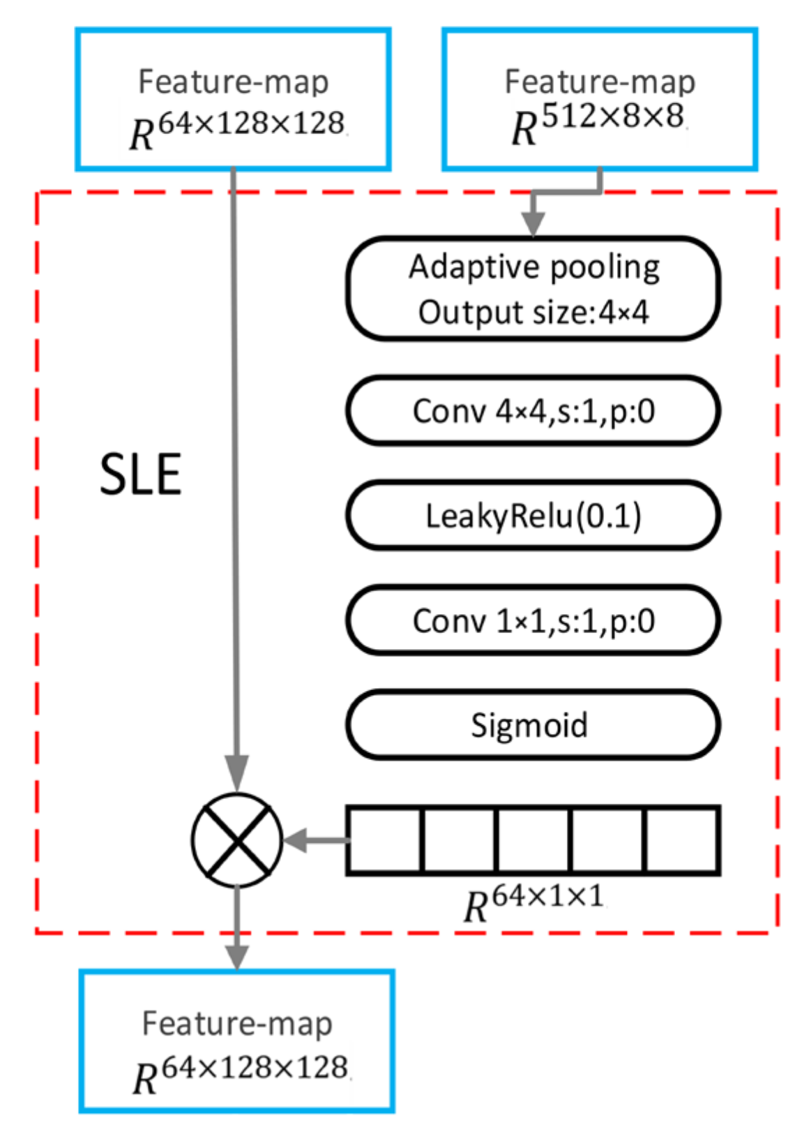
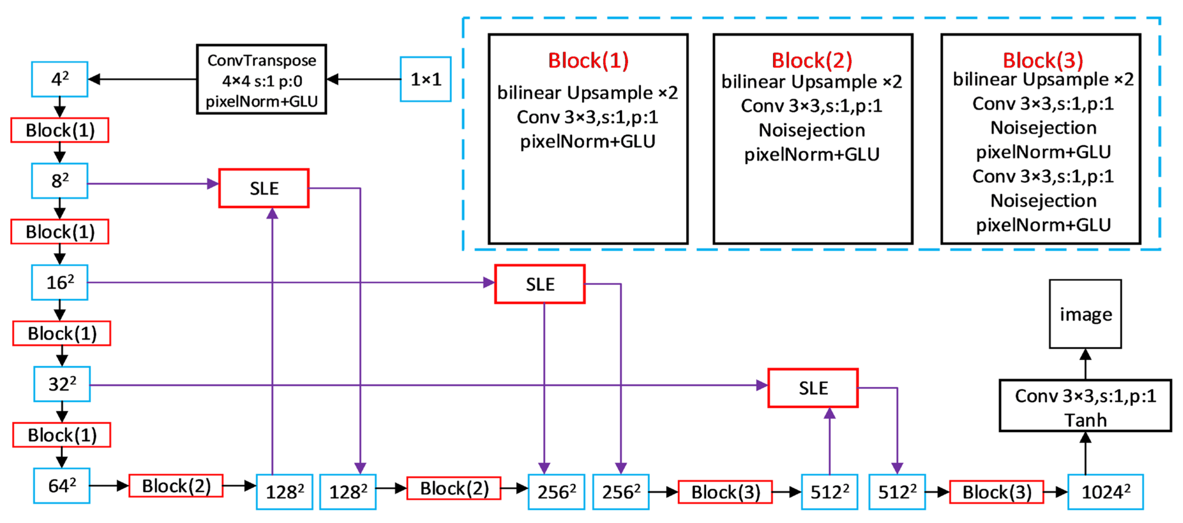
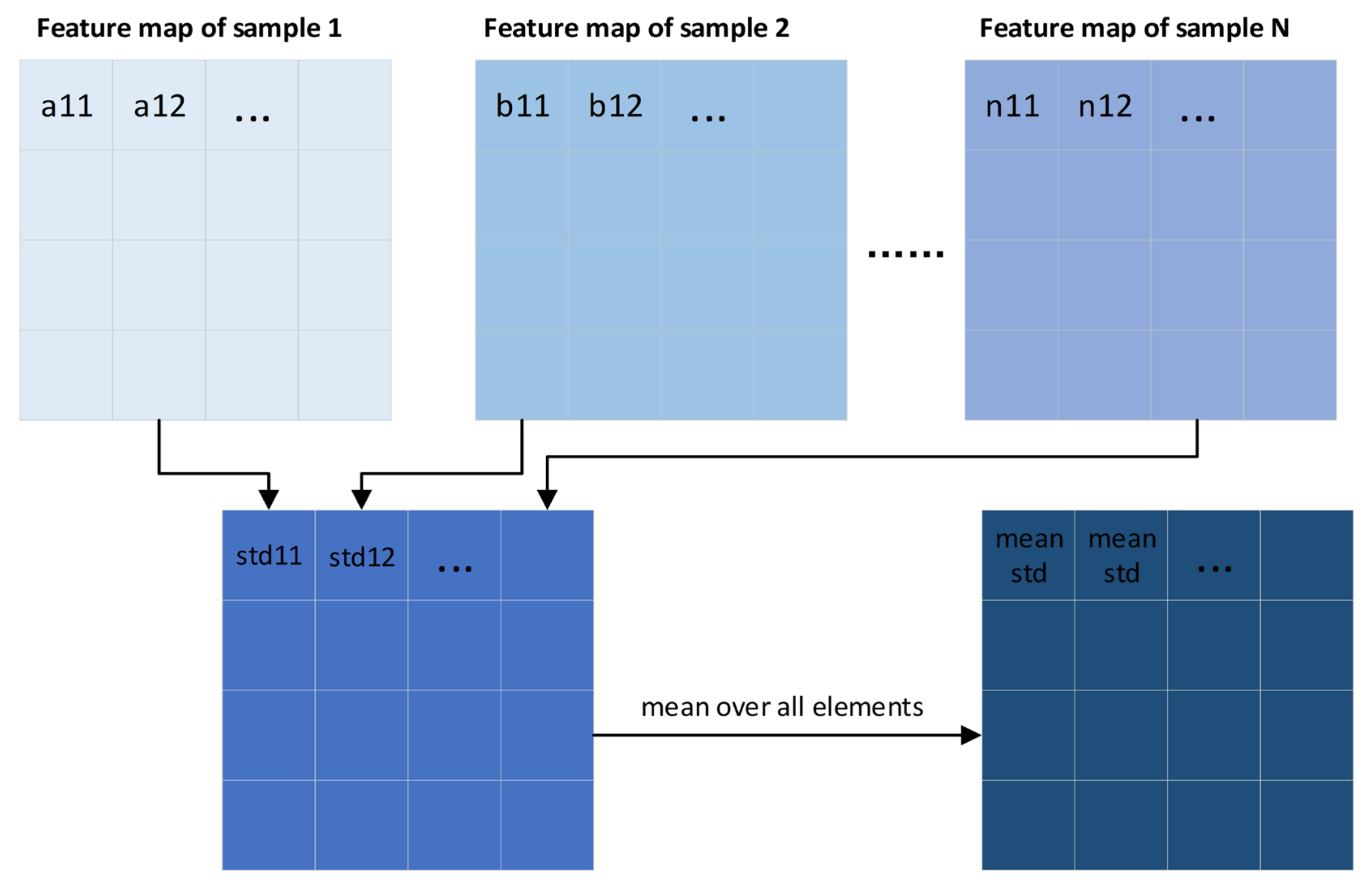
2.3. Improved FastGAN Model

When the FastGAN model is applied to citrus leaf disease sample generation, the generated image disease features are unclear. There is insufficient sample richness and a high repetition rate when several thousand images are generated using the trained model. To solve these problems and make the model more applicable to citrus disease sample generation, we improved FastGAN to propose the FastGAN2 model.
First, the structure of the original model generator was redesigned. The interpolation algorithm used in the original model upsampling is the Nearest Interpolation model, which has the fastest calculation speed; however, the effect is poor, and the generated image can easily produce jaggedness. We replaced it with the Bilinear model, which uses 4-pixel points in the original image to calculate the 1-pixel point in the new image to smoothen the generated image. Unlike the original model, which uses the same upsampling block for all layers, we used upsampling blocks with different strategies for different layers. The 42–322 layers representing rough features use a single convolutional layer, the 642–2562 layers representing fine features use a convolutional layer and a noise layer, and the 5122–10242 layers use two convolutional and two Noisejection layers. For all upsampling blocks, the PixelNorm layer replaces the BachNorm layer in the original model. The PixelNorm layer is demonstrated in Equation (2), and the improved generator structure is shown in Figure 4. The Noisejection layer was independently added to each pixel to control random changes.
b x , y = a x , y 1 N j = 0 N 1 a x , y j 2 + ϵ ,
In the formula, N is the number of feature maps, where a x , y and b x , y are, respectively, the original and normalized feature vectors in pixels ( x , y ) , ϵ = 10 8 . The PixelNorm layer normalizes each pixel point to avoid extreme weights of input noise and improve stability.
Because the FastGAN2 model training is performed on 50 images, it is easy to cause mode collapse and generate duplicate images when generating 2000 images. Karras, Aila, Laine, and Lehtinen [38] proposed a mini-batch standard deviation to increase the diversity of generated samples. To solve this problem, we added it at the end of the discriminator of the original model, as shown in Figure 5. The method divides a batch size image into X parts evenly, where each part contains batch size X images, and finds the standard deviation of each image’s feature map at different spatial locations; i.e., NumPy’s standard function is used to find the standard along the sample dimension. This results in a new feature map, which is then averaged over the feature map to obtain a value, and this value is expanded to the size of a feature map and stitched together with the original feature map as the input to the next layer, i.e., adding a statistical channel to each image.

2.4. Improved EfficientNet-B5

After comparing the classification performances of Densenet121, ResNet50, ShuffleNetv2, Mlp-Mixer, MobileNetv3, EfficientNet-B3, and EfficientNet-B5, we found that EfficientNet-B5 had the best performance (performance comparison can be found in Table 1). Therefore, we improve EfficientNet-B5 by using the AWP mechanism to add perturbations to model weights and inputs to increase the robustness of the model. We also used Arcface loss and added a cumulative corner margin between elements and target weights to enhance intra-class compactness and inter-class variability. Arcface is a loss function applied to face recognition, as proposed by Deng et al. [39], and it maximizes the classification boundaries in angular space and adds a cumulative angular margin between features and target weights to enhance intra-class compactness and inter-class differences.
Arcface was used instead of the softmax loss function because of the high similarity of various citrus leaf diseases. The softmax loss function formula is given by Equation (3):
L 1 = 1 N i = 1 N log e W y i T x i + b y i j = 1 n e W j T x i + b j ,
where x i denotes the deep feature of the ith sample associated with the category y i , j denotes the column of weight w , b j is the bias corresponding to w j , n is the number of categories, and N is the batch size.
The softmax loss function does not explicitly optimize the embedding function to achieve a higher similarity of samples within categories and a higher diversity of samples between categories. It is improved by first setting the bias b j to 0, and the inner product of the weights and inputs is expressed by Equation (4):
W j T x i = W j x i c o s θ j
Processing w j with L 2 regularization makes W j = 1, ( L 2 regularization is to divide each value in the w j vector by the modulus of w j separately to obtain the new w j , and the modulus of the new w j is 1).
Hence, Equation (5) can be obtained from Equation (3):
L 2 = 1 N i = 1 N log e x i cos ( θ y i ) e x i cos ( θ y i ) + + j = 1 , j y i n e x i cos θ j
input x i is also regularized with L 2 by multiplying by scale parameter s . The normalization step of the features and weights makes the prediction depend only on the angle between the features and weights. Thus, the learned embedding features were distributed on a hypersphere of radius s. Because the embedding features are distributed around the center of each feature on the hypersphere, a cumulative angular margin is added between x i and y i to enhance the intra-class compactness and inter-class variance [40], yielding Equation (6) for the Arcface:
L 3 = 1 N i = 1 N log e s ( cos ( θ y i + m ) ) e s ( cos ( θ y i + m ) ) + j = 1 , j y i n e scos θ j
To improve the generalization ability of the model, an adversarial training mechanism (AWP) proposed by Wu et al. [41] was used for EfficientNet-B5. Adversarial training introduces noise, which can regularize parameters and improve the robustness of the model. The weight loss landscape (WLL) is used to represent the standard generalization gap (the difference between the accuracy of the model on the training set and the accuracy of the test set) under standard training scenarios. As a result of the AWP limiting the flatness of the WLL in adversarial training, a dual perturbation mechanism is formed, that is, the adversarial perturbation input and weights. The original adversarial loss is given by Equation (7):
min w ρ ( w ) , ρ ( w ) = 1 n i = 1 n max x i x i p ϵ ( f w ( x i ) , y i )
where n is the number of training samples, x i is the adversarial sample within a ball (bounded by L p parameterization) centered on the natural sample x i , f w is the deep neural network (DNN) with weight w , l ( ) is the standard classification loss, such as cross-entropy loss, and ρ w is the adversarial loss.
The AWP algorithm flattens the WLL by injecting worst-case weight perturbations into a DNN. To improve the test robustness, investigators must focus on training robustness and the robustness generalization gap, as shown in Equation (8):
min w { ρ ( w ) + ( ρ ( w + V ) ρ ( w ) ) } min w ρ ( w + V )
where ρ w is the original adversarial loss in Equation (7), ρ w + V ρ w denotes the flatness of the WLL, and V is the perturbation weight that must be carefully chosen. Unlike the commonly used random weight perturbation (random direction sampling), the adversarial loss of the AWP is significantly increased, as demonstrated in Equation (9):
min w max V V ρ ( w + V ) min w max V V 1 n i = 1 n max x i x i p ϵ ( f w + V ( x i ) , y i ) ,
where V is the range of values of the perturbation weights V . The maximization of V depends on the entire instance to maximize the entire loss (not the loss of each instance); therefore, these two maximizations are not interchangeable.

3. Results and Discussion

3.1. Generate Image Quality Ratings

The training set Train-GAN was used to train FastGAN for approximately 2.5 h and FastGAN2 for approximately 3 h to complete the training of 30,000 epochs. The model was saved every 5000 epochs, and the images generated during the training process were saved every 1000 epochs.
T-SNE is a data dimensionality reduction and visualization method [42], which is an embedding model that can map data in a high-dimensional space to a low-dimensional space and preserve the local characteristics of the dataset. Therefore, when we want to classify a high-dimensional dataset, it is not clear whether this dataset has good separability (small intervals between similar classes and large intervals between distinct classes), and we can project the data into a 2- or 3-dimensional space for observation by T-SNE.
In this study, we reduced the dimensionality of the FastGAN2-generated images and the original images to observe their distribution in two-dimensional space. As demonstrated in Figure 6, where Figure 6A,B are the original images and generated images in the two-dimensional space distribution, respectively, by observing Figure 6A, it can be seen that the interval between the nutritional deficiency leaves and healthy leaves is a small boundary and is not clear, indicating that these two types of leaves do not exhibit a strong classification of difference; Figure 6B shows that the generated images also conform to this distribution. Figure 6C shows the fitting of the scatter plot between the generated and original images, the circle symbol representing the real image and the cross symbol representing the generated image overlap, which indicates that the four generated types of images are in the same distribution as the real image.
The FID is the distance between the generated and real images. A smaller distance indicates a well-generated image, that is, a sharp and diverse image. The FID is computed through the inception model, which removes the last fully connected layer of the inception model used for classification and outputs a 2048-dimensional vector from the previous layer. Here, inception no longer performs classification but feature extraction to obtain 2048-dimensional vectors, and each dimension represents some feature. N was taken for each of the generated and real images. After the transformed inception network, each obtains an N*2048-dimensional feature vector and then uses Equation (10) to calculate the distance between the two N*2048-dimensional feature vectors:
F I D = μ r μ g 2 + T r ( r + g 2 ( r g ) 1 / 2 ) ,
where μ r denotes the feature mean of the real image, μ g is the feature mean of the generated image, r is the covariance matrix of the real image, and g is the covariance matrix of the generated image.
KID is a GAN generation quality metric that is very similar to FID to assess the degree of GAN convergence [43], which does not require the assumption of a normal distribution of FID and is an unbiased estimation.
Table 2 summarizes the comparison of the FID and KID scores of FastGAN2 and FastGAN on the four types of leaves. The FID and KID scores of the four kinds of leaves generated by the FastGAN2 network are lower than those of the FastGAN network, indicating that the improved network generates images with better clarity and diversity.
Figure 7 compares the details of the citrus ulcer images generated by FastGAN2 and FastGAN. The images generated by the FastGAN network have unclear lesions, checkerboard artifacts on the midvein and tips, and the leaf contours are distorted (not continuous). The images generated by the FastGAN2 network are closer to the original images, and semantic information remains intact for the whole leaf and enlarged lesions, midvein, and leaf tips. Their color, texture, and contour features are more obvious.
Figure 8 shows the comparison between the image generated by FastGAN and FastGAN2 and the original image with the complex background. It can be seen from row B that the background of the image produced by FastGAN2 is very close to the original image, and the leaf contour and midvein transition are natural. However, it can be seen from the image generated by FastGAN in line C that the background of the image is seriously distorted, and there are problems such as distortion and unclear leaf contour. This indicates that FastGAN2 can also generate high-quality images of diseased citrus leaves under complex backgrounds.
Figure 9 compares the four types of citrus leaf images generated by FastGAN2 and FastGAN with the original images, and the FastGAN2 generated images are closer to the original images than those generated by FastGAN. Figure 10 shows some of the images in the dataset Train-CNN generated by the FastGAN2 network; the four generated types of citrus leaves match the detailed features of the real images, in which the traces of rain can be seen in the background of the generated images. There are reflections formed by water on the leaves as the real images of the ulcer leaves were taken on a rainy day.

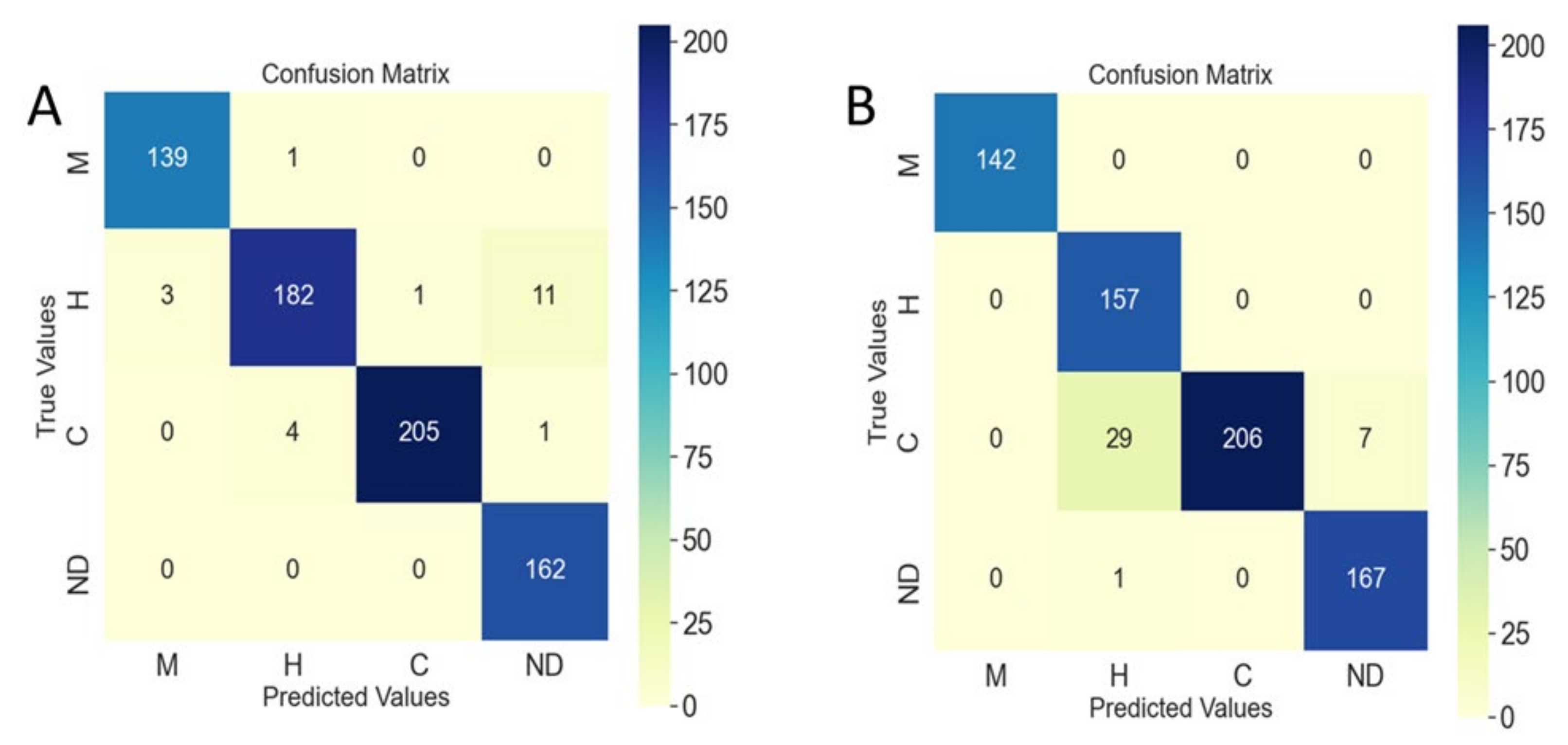
3.2. Classified Network Performance Evaluation

To verify whether the classification network trained using the images generated by the FastGAN2 network only can successfully recognize the captured images, we trained ten classification networks using the Train-CNN, the image dataset generated by the FastGAN2 network, and evaluated the classification network performance using Test-CNN as the test set with accuracy, recall, precision, and F1-score as the evaluation metrics. This is formulated in Equations (11)–(14):
A c c u r a c y = T P + T N T P + T N + F P + F N ,
Recall = T P T P + F N ,
Precision = T P T P + F P ,
F 1 - score = 2 Precision Recall     Precision   +   Recall   ,
where T P is the number of samples with a true positive value and positive prediction, F P is the number of samples with a true negative value but positive prediction, F N is the number of samples with a true positive value but negative prediction, and T N is the number of samples with a true negative value and negative prediction.
In this study, the images generated by FastGAN and Train-CNN are, respectively, used as training sets to train the classification network; Test-CNN was used as the test set to evaluate the performance of the classification network. It can be seen from Table 3 that the accuracy, precision, recall and F1-score achieved by using FastGAN2 to generate images for training ten classification networks are higher than those achieved by FastGAN. Among them, EfficientNet-B5 has the highest score in each item, which is higher than the average.
The confusion matrix in Figure 11 shows that EfficientNet-B5-pro has better generalization and robustness [44]. It can be seen from Figure 11A that EfficientNet-B5-pro judges that the largest number of errors is within the nutritional deficiency leaves, as it misjudges 11 nutritional deficiency leaves as healthy leaves. According to the previous T-SNE results, it can be seen that this may be due to the higher similarity between healthy and nutritional deficiency leaves. Compared with Figure 11B, it can be seen that the unimproved EfficientNet-B5 misclassifies more healthy leaves, while EfficientNet-B5-Pro has similar discrimination rates for four kinds of leaves, indicating that the improved EfficientNet-B5 has better intra-class compactness and inter-class difference.
Table 4 depicts the classification results of EfficientNet-B5-pro for four kinds of leaves. The nutritional deficiency leaves were divided into two separate groups (zinc and magnesium deficiency). In this table, the average score for healthy leaves is the lowest and that for nutritionally deficient leaves is the second lowest. This may be due to the high similarity and small differences between healthy leaves and nutritionally deficient leaves, which makes classification difficult. It can also be seen from the previously mentioned T-SNE reduced dimensional visualization method that the boundaries between healthy and deficient leaves are not clear in the scatter plot. Figure 12 shows the training loss and test accuracy curves of the EfficientNet-B5-pro model.

4. Conclusions

In this study, we generated citrus disease and nutritional deficiency phenotype data using the FastGAN2 network, trained the classification network using only the generated images, and achieved high accuracy on the shot dataset. The impact on the performance of classification networks when the training and test sets are from different regions is addressed, and the generalization and robustness of classification networks in citrus disease and nutritional deficiency leaf identification are improved. Compared to most GAN methods for generating plant disease samples, this study does not require pairs of data, no background must be removed, and only a small amount of data is required to complete the training of the GAN network. Through the model proposed in this paper, high-quality citrus disease and nutritional deficiency images are successfully generated. After training the classification network solely by using the images generated in this paper, citrus disease and nutritional deficiency images in a real environment can be successfully identified with high accuracy. Although this study was conducted for citrus diseases, the method used can also provide new ideas for the classification and identification of other plant diseases where samples are not sufficient. In the future, we will develop a mobile application that will deploy the algorithms mentioned in this article to a website or software to help fruit farmers identify citrus disease.

Author Contributions

Data curation, Y.W. and Z.C.; project administration, S.L.; resources, S.S. and D.S.; supervision, Z.L.; writing—original draft, Y.G.; writing—review and editing, Q.D. All authors have read and agreed to the published version of the manuscript.

Funding

This research was funded by the National Natural Science Foundation of China (grant No. 31971797). This study was also partly supported by the China Agriculture Research System of MOF and MARA (grant No. CARS-26) and the Guangdong Provincial Special Fund for Modern Agriculture Industry Technology Innovation Teams (grant No. 2022KJ108, No. 2023KJ108).

Institutional Review Board Statement

Not applicable.

Data Availability Statement

Not applicable.

Conflicts of Interest

The authors declare no conflict of interest.

Abbreviations

ArcfaceAdaptive angular margin
FIDFréchet inception distance
KIDKernel inception distance
GANGenerative adversarial network
G Generator
SLESkip-layer excitation
DNNDeep neural network
WLLWeight loss landscape
APAverage precision
CNNConvolutional neural network
AWPAdversarial weight perturbation
AdamAdaptive moment estimation

References

  1. Iqbal, Z.; Khan, M.A.; Sharif, M.; Shah, J.H.; Rehman, M.H.U.; Javed, K. An automated detection and classification of citrus plant diseases using image processing techniques. Comput. Electron. Agric. 2018, 153, 12–32. [Google Scholar] [CrossRef]
  2. Gulzar, Y. Fruit Image Classification Model Based on MobileNetV2 with Deep Transfer Learning Technique. Sustainability 2023, 15, 1906. [Google Scholar] [CrossRef]
  3. Palei, S.; Behera, S.K.; Sethy, P.K. A Systematic Review of Citrus Disease Perceptions and Fruit Grading Using Machine Vision. Procedia Comput. Sci. 2023, 218, 2504–2519. [Google Scholar] [CrossRef]
  4. Mamat, N.; Othman, M.F.; Abdulghafor, R.; Alwan, A.A.; Gulzar, Y. Enhancing Image Annotation Technique of Fruit Classification Using a Deep Learning Approach. Sustainability 2023, 15, 901. [Google Scholar] [CrossRef]
  5. Wu, F.Y.; Duan, J.L.; Ai, P.Y.; Chen, Z.Y.; Yang, Z.; Zou, X.J. Rachis detection and three-dimensional localization of cut off point for vision-based banana robot. Comput. Electron. Agric. 2022, 198, 107079. [Google Scholar] [CrossRef]
  6. Wu, F.Y.; Duan, J.L.; Chen, S.Y.; Ye, Y.X.; Ai, P.Y.; Yang, Z. Multi-Target Recognition of Bananas and Automatic Positioning for the Inflorescence Axis Cutting Point. Front. Plant. Sci. 2021, 12, 705021. [Google Scholar] [CrossRef]
  7. Tang, Y.C.; Zhou, H.; Wang, H.J.; Zhang, Y.Q. Fruit detection and positioning technology for a Camellia oleifera C. Abel orchard based on improved YOLOv4-tiny model and binocular stereo vision. Expert Syst. Appl. 2023, 211, 118573. [Google Scholar] [CrossRef]
  8. Da Silva, J.C.F.; Silva, M.C.; Luz, E.J.S.; Delabrida, S.; Oliveira, R.A.R. Using Mobile Edge AI to Detect and Map Diseases in Citrus Orchards. Sensors 2023, 23, 2165. [Google Scholar] [CrossRef]
  9. Kamilaris, A.; Prenafeta-Boldu, F.X. Deep learning in agriculture: A survey. Comput. Electron. Agric. 2018, 147, 70–90. [Google Scholar] [CrossRef] [Green Version]
  10. Zhang, S.W.; Wu, X.W.; You, Z.H.; Zhang, L.Q. Leaf image based cucumber disease recognition using sparse representation classification. Comput. Electron. Agric. 2017, 134, 135–141. [Google Scholar] [CrossRef]
  11. Liu, H.Y.; Jiao, L.; Wang, R.J.; Xie, C.J.; Du, J.M.; Chen, H.B.; Li, R. WSRD-Net: A Convolutional Neural Network-Based Arbitrary-Oriented Wheat Stripe Rust Detection Method. Front. Plant. Sci. 2022, 13, 876069. [Google Scholar] [CrossRef] [PubMed]
  12. Zhong, Y.; Zhao, M. Research on deep learning in apple leaf disease recognition. Comput. Electron. Agric. 2020, 168, 105146. [Google Scholar] [CrossRef]
  13. Yao, N.; Ni, F.; Wang, Z.; Luo, J.; Sung, W.K.; Luo, C.; Li, G. L2MXception: An improved Xception network for classification of peach diseases. Plant Methods 2021, 17, 36. [Google Scholar] [CrossRef] [PubMed]
  14. Chollet, F. Xception: Deep Learning with Depthwise Separable Convolutions in Computer Vision and Pattern Recognition. In Proceedings of the IEEE Conference on Computer Vision and Pattern Recognition (CVPR), Honolulu, HI, USA, 21–26 July 2017. [Google Scholar]
  15. Janarthan, S.; Thuseethan, S.; Rajasegarar, S.; Lyu, Q.; Zheng, Y.Q.; Yearwood, J. Deep Metric Learning Based Citrus Disease Classification with Sparse Data. IEEE Access 2020, 8, 162588–162600. [Google Scholar] [CrossRef]
  16. Salman, S.; Liu, X. Overfitting Mechanism and Avoidance in Deep Neural Networks. arXiv 2019, arXiv:1901.06566v1. [Google Scholar]
  17. Li, W.; Chen, C.; Zhang, M.M.; Li, H.C.; Du, Q. Data Augmentation for Hyperspectral Image Classification with Deep CNN. IEEE Geosci. Remote Sens. Lett. 2019, 16, 593–597. [Google Scholar] [CrossRef]
  18. Goodfellow, I.; Pouget-Abadie, J.; Mirza, M.; Xu, B.; Warde-Farley, D.; Ozair, S.; Courville, A.; Bengio, Y. Generative Adversarial Nets. In Proceedings of the 28th Conference on Neural Information Processing Systems, Montréal, QC, Canada, 8–13 August 2014. [Google Scholar]
  19. You, C.; Li, G.; Zhang, Y.; Zhang, X.; Shan, H.; Li, M.; Ju, S.; Zhao, Z.; Zhang, Z.; Cong, W.; et al. CT Super-Resolution GAN Constrained by the Identical, Residual, and Cycle Learning Ensemble (GAN-CIRCLE). IEEE Trans. Med. Imaging 2020, 39, 188–203. [Google Scholar] [CrossRef] [Green Version]
  20. Lin, Y.; Li, Y.; Cui, H.; Feng, Z. WeaGAN: Generative Adversarial Network for Weather Translation of Image among Multi-domain. In Proceedings of the International Conference on Behavioral, Economic and Socio-Cultural Computing, Beijing, China, 28–30 October 2019. [Google Scholar]
  21. Niu, S.L.; Li, B.; Wang, X.G.; Lin, H. Defect Image Sample Generation with GAN for Improving Defect Recognition. IEEE Trans. Automat. Sci. Eng. 2020, 17, 1611–1622. [Google Scholar] [CrossRef]
  22. Ma, L.; Shuai, R.; Ran, X.; Liu, W.; Ye, C. Combining DC-GAN with ResNet for blood cell image classification. Med. Biol. Eng. Comput. 2020, 58, 1251–1264. [Google Scholar] [CrossRef]
  23. Cap, Q.H.; Uga, H.; Kagiwada, S.; Iyatomi, H. LeafGAN: An Effective Data Augmentation Method for Practical Plant Disease Diagnosis. IEEE Trans. Automat. Sci. Eng. 2020, 9, 1258–1267. [Google Scholar] [CrossRef]
  24. Xiao, D.Q.; Zeng, R.L.; Liu, Y.F.; Huang, Y.G.; Liu, J.B.; Feng, J.Z.; Zhang, X.L. Citrus greening disease recognition algorithm based on classification network using TRL-GAN. Comput. Electron. Agric. 2022, 200, 107206. [Google Scholar] [CrossRef]
  25. Karras, T.; Laine, S.; Aittala, M.; Hellsten, J.; Lehtinen, J.; Aila, T. Analyzing and Improving the Image Quality of StyleGAN. In Proceedings of the IEEE/CVF Conference on Computer Vision and Pattern Recognition (CVPR), Seattle, WA, USA, 13–19 June 2020. [Google Scholar]
  26. Karras, T.; Laine, S.; Aila, T. A Style-Based Generator Architecture for Generative Adversarial Networks. IEEE Trans. Pattern Anal. Mach. Intell. 2019, 43, 4217–4228. [Google Scholar] [CrossRef] [PubMed] [Green Version]
  27. Liu, B.; Zhu, Y.; Song, K.; Elgammal, A. Towards Faster and Stabilized GAN Training for High-fidelity Few-shot Image Synthesis. In Proceedings of the IEEE/CVF Conference on Computer Vision and Pattern Recognition, Online, 19–25 June 2021. [Google Scholar]
  28. Mohanty, S.P.; Hughes, D.P.; Salathe, M. Using Deep Learning for Image-Based Plant Disease Detection. Front. Plant. Sci. 2016, 7, 1419. [Google Scholar] [CrossRef] [PubMed] [Green Version]
  29. Ferentinos, K.P. Deep learning models for plant disease detection and diagnosis. Comput. Electron. Agric. 2018, 145, 311–318. [Google Scholar] [CrossRef]
  30. Ma, N.; Zhang, X.; Zheng, H.-T.; Sun, J. ShuffleNet V2: Practical Guidelines for Efficient CNN Architecture Design. In Proceedings of the IEEE/CVF Conference on Computer Vision and Pattern Recognition, Salt Lake City, UT, USA, 18–23 June 2018. [Google Scholar]
  31. Tolstikhin, I.; Houlsby, N.; Kolesnikov, A.; Beyer, L.; Zhai, X.; Unterthiner, T.; Yung, J.; Steiner, A.; Keysers, D.; Uszkoreit, J.; et al. MLP-Mixer: An all-MLP Architecture for Vision. In Proceedings of the IEEE/CVF Conference on Computer Vision and Pattern Recognition, Online, 19–25 June 2021. [Google Scholar]
  32. Howard, A.; Sandler, M.; Chu, G.; Chen, L.-C.; Chen, B.; Tan, M.; Wang, W.; Zhu, Y.; Pang, R.; Vasudevan, V.; et al. Searching for MobileNetV3. In Proceedings of the IEEE/CVF International Conference on Computer Vision, Seoul, Republic of Korea, 27 October–2 November 2019. [Google Scholar]
  33. Tan, M.; Le, Q.V. EfficientNet: Rethinking Model Scaling for Convolutional Neural Networks. In Proceedings of the International Conference on Machine Learning, Long Beach, CA, USA, 9–15 June 2019. [Google Scholar]
  34. Kaggle. CCL’20|Kaggle. Available online: https://www.kaggle.com/datasets/downloader007/ccl20 (accessed on 23 August 2022).
  35. Loshchilov, I.; Hutter, F. SGDR: Stochastic Gradient Descent with Warm Restarts. In Proceedings of the International Conference on Learning Representations, Toulon, France, 24–26 April 2017. [Google Scholar]
  36. Loshchilov, I.; Hutter, F. Decoupled Weight Decay Regularization. In Proceedings of the International Conference on Learning Representations, New Orleans, LA, USA, 6–9 May 2019. [Google Scholar]
  37. He, K.; Zhang, X.; Ren, S.; Sun, J. Deep Residual Learning for Image Recognition. In Proceedings of the IEEE Conference on Computer Vision and Pattern Recognition, Boston, MA, USA, 7–12 June 2015. [Google Scholar]
  38. Karras, T.; Aila, T.; Laine, S.; Lehtinen, J. Progressive Growing of GANS for Improved Quality, Stability, and Variation. arXiv 2018, arXiv:1710.10196. [Google Scholar]
  39. Deng, J.; Guo, J.; Xue, N.; Zafeiriou, S. ArcFace: Additive Angular Margin Loss for Deep Face Recognition. In Proceedings of the IEEE/CVF Conference on Computer Vision and Pattern Recognition, Long Beach, CA, USA, 15–20 June 2019. [Google Scholar]
  40. Xu, Q.; Huang, G.; Yuan, Y.; Guo, C.; Sun, Y.; Wu, F.; Weinberger, K. An empirical study on evaluation metrics of generative adversarial networks. arXiv 2018, arXiv:1806.07755. [Google Scholar]
  41. Wu, D.; Xia, S.-T.; Wang, Y. Adversarial Weight Perturbation Helps Robust Generalization. In Proceedings of the Advances in Neural Information Processing Systems 33: Annual Conference on Neural Information Processing Systems, Online, 6–12 June 2020. [Google Scholar]
  42. Arora, S.; Hu, W.; Kothari, P.K. An Analysis of the t-SNE Algorithm for Data Visualization. PlMR 2018, 75, 1455–1462. [Google Scholar]
  43. Bińkowski, M.; Sutherland, D.J.; Arbel, M.; Gretton, A. Demystifying MMD GANs. arXiv 2018, arXiv:1801.01401. [Google Scholar]
  44. Luque, A.; Carrasco, A.; Martín, A.; de las Heras, A. The impact of class imbalance in classification performance metrics based on the binary confusion matrix. Pattern Recognit. 2019, 91, 216–231. [Google Scholar] [CrossRef]
Figure 1. The four kinds of leaves used in the experiment: (A,E) canker, (B,F) melanose, (C,G) healthy, (D) magnesium deficiency, and (H) zinc deficiency; (AD) is simple background, (EH) is complicated background.
Agronomy 13 00988 g001
Figure 2. Framework flowchart of generation and classification. Dataset A is divided into Train-GAN and Test-CNN. Train-GAN is used to train FastGAN and FastGAN2. The trained FastGAN2 generates Train-CNN as the training set of CNN and Test-CNN as the tFest set. T-SNE is used to evaluate the quality of Train-CNN. FIID and KID are used to compare the ability of FastGAN and FastGAN2 to generate images.
Agronomy 13 00988 g002
Figure 3. SLE module structure. Feature maps at 8 × 8 and 128 × 128 are, respectively, x low   and x h i g h in Equation (1). All the black boxes are used to change the size of x low   .
Agronomy 13 00988 g003
Figure 4. The redesigned generator structure. The blue dotted line frame contains three different upsample blocks. The blue solid line frame represents the size of the feature map, while the red solid line frame represents the SLE module in Figure 3.
Agronomy 13 00988 g004
Figure 5. The minibatch standard deviation flow chart. Feature map1, 2… N is divided equally into multiple parts and finds the standard deviation of each image’s feature map at different spatial locations. This results in a new feature map, which is then averaged over the feature map to obtain a value, and this value is expanded to the size of a feature map.
Agronomy 13 00988 g005
Figure 6. Scatter plot of T-SNE after dimensionality reduction: the circles are the real dataset; the crosses are the fake dataset. Red = melanose; dark-green = healthy; light green = nutritional deficiency; blue = canker. (A) only real dataset; (B) only fake dataset; (C) combination of real and fake dataset.
Agronomy 13 00988 g006
Figure 7. “Real image”, “FastGAN2”, and “FastGAN” images down the sides and “Leaf”, “Lesion”, “Midvein”, and “Leaf tip” images across the top.
Agronomy 13 00988 g007
Figure 8. Comparison between the image generated by FastGAN and FastGAN2 and the original image with the complex background: “Real image”, “FastGAN2” and “FastGAN” images down the sides.
Agronomy 13 00988 g008
Figure 9. Comparison of four kinds of citrus leaf images generated by FastGAN and FastGAN2 with real images: (A) real dataset; (B) images generated by FastGAN2; (C) images generated by FastGAN.
Agronomy 13 00988 g009
Figure 10. A portion of the dataset generated by FastGAN2: (A) healthy; (B) nutritional deficiency; (C) canker; (D) melanose.
Agronomy 13 00988 g010
Figure 11. Confusion Matrix: (A) EfficientNet-B5-pro; (B) EfficientNet-B5. “M” = melanose; “H” = healthy; “C” = canker; “ND” = nutritional deficiency.
Agronomy 13 00988 g011
Figure 12. Training loss and test accuracy of the EfficientNet-B5-pro model.
Agronomy 13 00988 g012
Table 1. The number of different species of leaves in each dataset.
LeavesTrain-GANTrain-CNNTest-CNN
Melanose502000142
Healthy502000187
Canker502000206
Nutritional Deficiency502000174
Table 2. Comparison of FID and KID scores of FastGAN2 and FastGAN on four kinds of leaves.
LeavesFastGAN2FastGAN
FIDKIDFIDKID
Melanose64.733.01153.5213.79
Healthy73.902.1890.984.71
Canker55.532.2164.593.01
Nutritional Deficiency53.562.0354.152.01
Average61.932.3690.815.88
Table 3. Performance comparison of ten kinds of classification networks.
NetworkAccuracy%Precision%Recall%F1-Score%
FastGanFastGan2FastGanFastGan2FastGanFastGan2FastGanFastGan2
Densenet12182.6490.9788.9593.7974.2191.3172.0391.61
Shufflenetv280.2194.6483.1594.4170.7194.4170.5894.37
Mlp Mixer82.3394.2293.0495.2073.8394.1273.0994.47
MobileNetV382.2992.8192.6394.1373.8792.4972.9893.06
ResNet5080.5691.2689.9993.6571.7091.5669.3391.86
Vision Transformer88.5493.9789.5294.5281.1594.0183.4794.04
Swin Transformer88.6293.4273.8795.1971.1793.6171.7393.88
EfficientNet-B386.1192.1086.0594.1280.3392.3477.1592.63
EfficientNet-B590.6294.7895.1596.1386.3494.9888.5295.23
EfficientNet-B5-pro94.6497.0495.3397.3294.7596.9694.8497.09
Average85.6693.5288.7694.8677.8093.5877.3793.82
Table 4. EfficientNet-B5-pro classification result.
LeavesF1-Score%Precision%Recall%Average%
Melanose98.5899.2997.8998.59
Healthy94.7992.3997.3394.84
Canker98.5697.6299.5198.56
Zinc Deficiency95.9297.929495.95
Magnesium Deficiency96.9399.394.6796.97
Disclaimer/Publisher’s Note: The statements, opinions and data contained in all publications are solely those of the individual author(s) and contributor(s) and not of MDPI and/or the editor(s). MDPI and/or the editor(s) disclaim responsibility for any injury to people or property resulting from any ideas, methods, instructions or products referred to in the content.

