
Modeling the Kinematic Response of Rice under Near-Ground Wind Fields Using the Finite Element Method

1
College of Engineering, South China Agricultural University, Guangzhou 510642, China
2
Rice Research Institute, Guangdong Academy of Agricultural Sciences, Guangzhou 510640, China
*
Author to whom correspondence should be addressed.
Agronomy 2023, 13(4), 1178; https://doi.org/10.3390/agronomy13041178
Submission received: 29 March 2023
/
Revised: 16 April 2023
/
Accepted: 19 April 2023
/
Published: 21 April 2023
(This article belongs to the Special Issue Development of Crop Protection Mechanical Engineering Technology, Evaluation of Efficacy and Safety of Pesticide Spraying)
Abstract
:Plant protection drones are commonly encountered in agricultural fields. Their downwash airflow can agitate flexible crops (e.g., rice and wheat) or even cause wind-induced losses. To predict the wind-induced responses of rice under wind fields, herein, a wind-induced rice response model (RWRM) was proposed using the finite element method. With the RWRM, the rice displacement and critical wind speed (CWS) were calculated at different wind speeds, considering the morphological and mechanical properties of rice, and the accuracy was experimentally verified and compared to that of an existing model. The results indicated that the mean paired difference and mean error in rice displacement amplitude prediction under 2~5 m/s wind speeds were 13.48 mm and 42.46 mm, respectively, and the predicted and measured values were highly correlated at the 1% significance level. Moreover, the CWS values for four rice species could be calculated with the model with an average of 3.57 m/s, and the difference between the simulated and theoretical values was 0.368. The strength of the wind-induced rice responses was primarily correlated with the mechanical properties, and to a lesser extent the morphology. The rice yield has a negative correlation with rice responses. Within a certain range, a bigger displacement and lower CWS could result in a higher rice yield. The RWRM achieved favorable modeling accuracy for the wind-induced responses of rice and could provide a simulation reference for balancing the wind-induced loss and rice yield.
1. Introduction
Rice feeds more than half of the population as one of the world’s top three food crops, and China produced 213.61 million tons of rice in 2020 (28.23% of the total rice production) [1,2]. Winds in fields, including natural winds and rotary winds originating from agricultural drones, closely influence the morphology and physiology of crops with pliable culms, as well as their final yields [3,4].
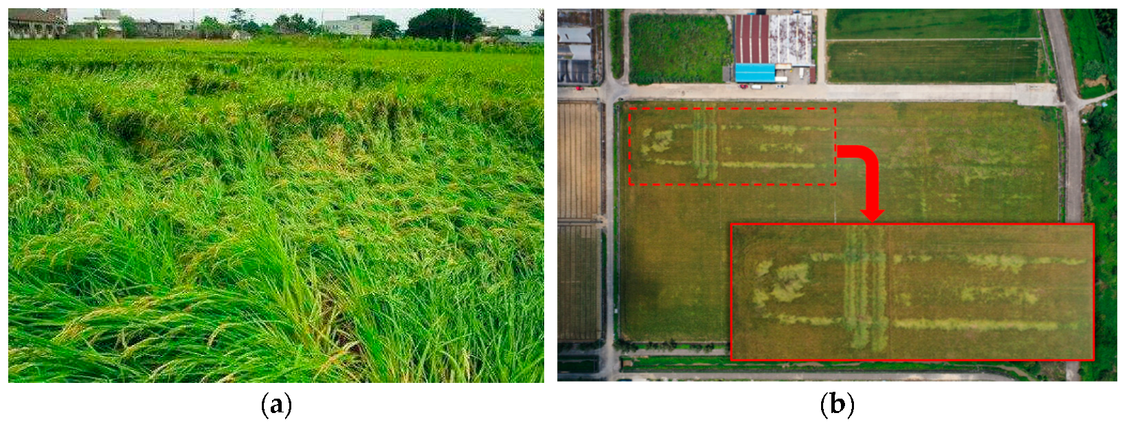
At the spike stage of rice, natural winds tend to induce stem bending and stem breakage (Figure 1a) [5], and crop tilting at 45° may result in an 18% yield reduction [6]. In the agriculture 4.0 era, agricultural drones are widely used in crop fields for spraying and fertilizing to improve the agricultural production efficiency [7,8]. During plant protection operations in paddy fields, the powerful downwash airflow produced by agricultural drones creates a restorable vortex patch in the rice canopy, which differs from the sway and tilt caused by natural winds. Guo et al. [9] found that the canopy vortex patch could increase the spray deposition by up to 5–7 times over non-vortex conditions. However, if the airflow intensity exceeds the critical stress of rice, this may result in a canopy vortex track across the rice canopy (Figure 1b).
The previous research on wind–crop interactions has mainly focused on kinematics. Finnigan [10] obtained the vertical profile characteristics of wheat canopy fluctuations under the influence of wind using a latitude and longitude measurement instrument and found that peak canopy fluctuations were correlated with the stalk vibration height. Previous studies [11,12] adopted a high-speed camera to record wind–alfalfa interactions and [13] used multiple cameras to record maize, oats, and oil seed rape. The field trial results have helped to validate theoretical calculations [14]. With the development of numerical computation, considerable research has been performed regarding the kinetics of wind–crop interactions. With the finite element method, a continuous system with infinite degrees of freedom can be transformed into a discrete system with finite degrees of freedom [15]. Yang et al. [16] simulated tree losses at different wind speeds with a finite element model of a pine tree. In this study, a single wind-induced rice response model (RWRM) was established based on the finite element method. We compared the variations in displacement between the simulation results and actual measurements to analyze the model accuracy and employed the model to calculate the critical wind speed (CWS) values of four rice varieties. The CWS, as an assessment indicator of the crop wind resistance, refers to the minimum ambient wind speed that can cause crop lodging, which can be mechanically deduced [13,17,18]. For an isolated plant, the generalized lodging model (GLM) is notable and applicable [19]. For instance, Wang et al. [20] assessed the effect of CWS-induced inversion on the quinoa yield using a finite element model of quinoa.
We examined the relationship between the wind-induced response characteristics and rice yield concerning biological (morphological and mechanical) characteristics to provide a simulation reference for balancing the rice yield and wind fall resistance requirements.
2. Materials and Methods
To establish a finite element model of the wind response of rice, the tested rice varieties and rice fields and the measured main biological characteristics of rice are introduced in Section 2.1 and Section 2.2, respectively. In Section 2.3, a finite element model of the rice–wind field is constructed based on the biological characteristics. In Section 2.4.1, the rice kinematic response under a horizontal wind field is simulated and validated. The CWS is calculated in Section 2.4.2.
2.1. Tested Rice and Paddy Field
Four representative rice species of the South China Rice Cultivation Area (Table 1) were selected as subjects.
The paddy fields are located in the Baiyun base of the Guangdong Academy of Agricultural Science (Guangzhou, Guangdong, China, longitude 113° E, latitude 23° N), in acidic light loam with an organic matter content of 23 g/kg, and the average altitude is 15 m. Moreover, the average annual summer temperature range is 25~32 °C, and the average annual rainfall reaches 916 mm. The irrigation conditions are satisfactory. The base, tiller, and spike fertilizers were applied at a ratio of 5:3:2, and the ratio of nitrogen, phosphorus, and potassium was 1:0.3:1. A Kestral NK5500 (Boothwyn, PA, USA) weather station was applied to record wind speed data for the paddy fields during the rice-growing period, and the maximum wind speed in these fields generally remained below 7 m/s, while the average wind speed reached 1.54 m/s, ranging 0–3.3 m/s. We collected 10–15 rice plants as samples along the diagonal in each field at the full heading stage and covered them with plastic film to prevent tissue damage during transportation.
2.2. Rice Biological Characteristics Measurements
2.2.1. Agronomic
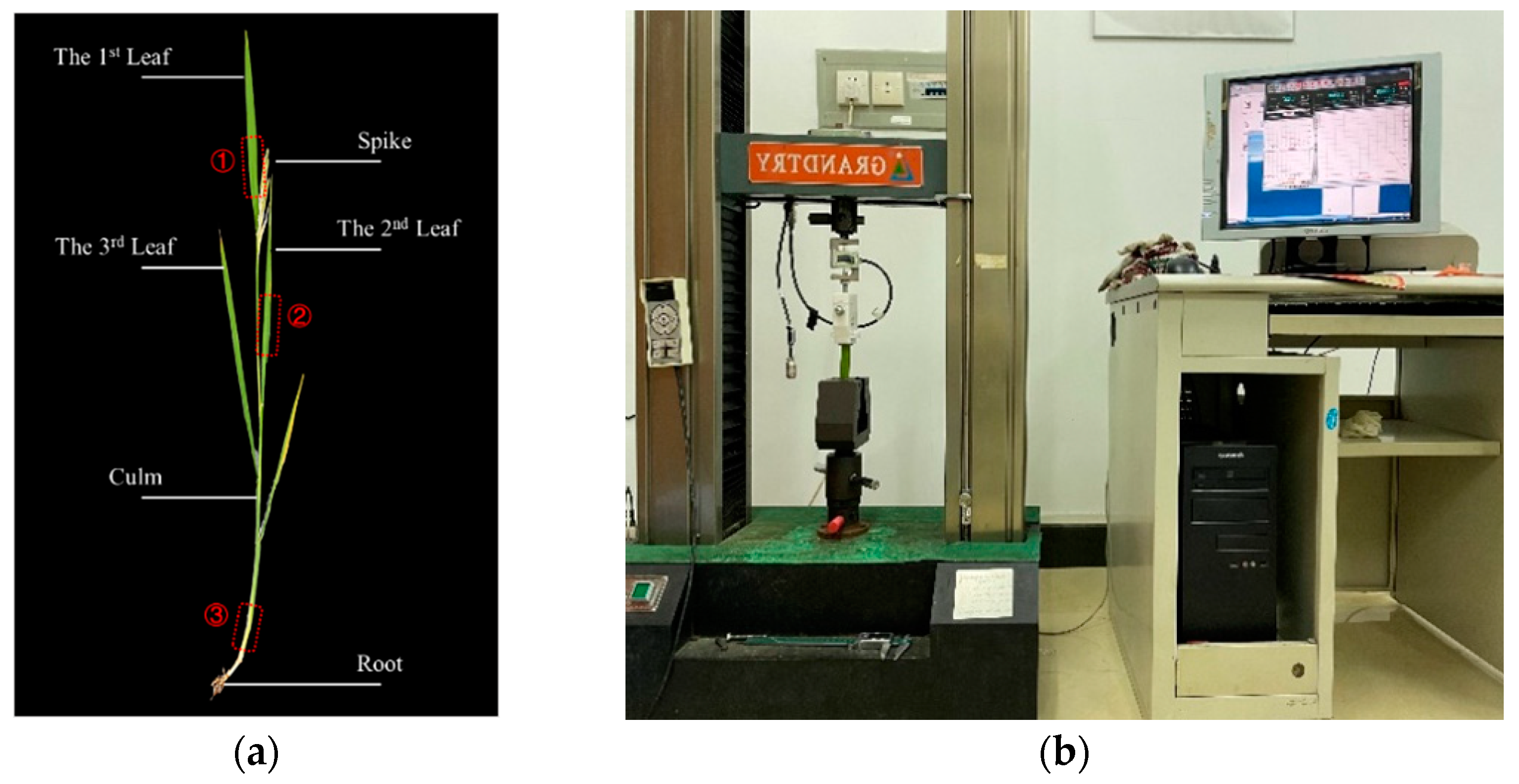
The agronomic characteristics of rice include the morphology, moisture content, and yield. The morphology was considered to build a geometric model of rice, and the moisture content and yield were employed to verify the practical significance of the RWRM. Rice spikes, culms, and leaves were considered and measured, including the spike weight ms, spike length , plant height , culm length , culm diameter , and wall thickness at 0.1 m from the root and the leaf length , leaf width , and leaf angle of the upper three leaves (please refer to Table 2 and Figure 2a).
To measure the wet basis moisture content of the rice, fresh culms with leaf sheaths and rice leaves were first weighed separately to obtain the wet weight m1. Then, they were placed in an oven in paper envelopes and maintained at 105 °C for 30 min. Finally, they were dried at 75 °C to a constant weight and the dry weight m2 was obtained. The moisture content can be calculated as follows:
After the rice had matured, we measured the mass (g) of the rice per 50 × 3 plants, adopting the average as the final yield of each species. We also present the estimated thousand grain weights of the corresponding rice species to show the differences between the species themselves.
2.2.2. Mechanical Tests
To obtain the rice material parameters needed in the finite element model and to calculate the mechanical parameters of rice, we conducted a uniaxial tensile test to obtain Young’s modulus (, GPa) values of rice culms and leaves from the stress–strain curve and a three-point bending test to calculate the bending force (, N), bending strength (, MPa), and bending energy (, mJ) of the rice culms. Both mechanical tests were performed on a universal testing machine (Guangzhou Guangcai Testing Instruments Co., Ltd., Guangzhou, China) (Figure 2b) equipped with a VISHAY STC 100-kg tensile load cell with an accuracy of 0.01 N. Each group of tests involving each species was repeated 5–8 times. Note that the culm tensile specimens were long rectangular strips dissected along the outer diameter of the culm. The specimens and test setup details are summarized in Table 3.
The uniaxial tensile test can provide the engineering stress ( = ) and strain ( = ), where is the loading force in N; is the initial cross-sectional area of the specimen in m2; is the specimen deformation in m; and is the specimen gauge length in m. The true stress and strain can be corrected via Equations (2) and (3), respectively:
where is the instantaneous cross-sectional area of the specimen in m2 and is the instantaneous length of the specimen in m.
Therefore, the Young’s modulus values of rice culms and the 1st and 2nd leaves can be calculated as follows (within the 0.05–2.00% elastic strain range):
The rice density ( = , kg/m3) was measured via the drainage method, where is the drainage volume and is the fresh weight of rice. Poisson’s ratio was retrieved from the literature. In summary, the RWRM material parameters involved are listed in Table 4.
2.3. Finite Element Model of Single Rice Setup
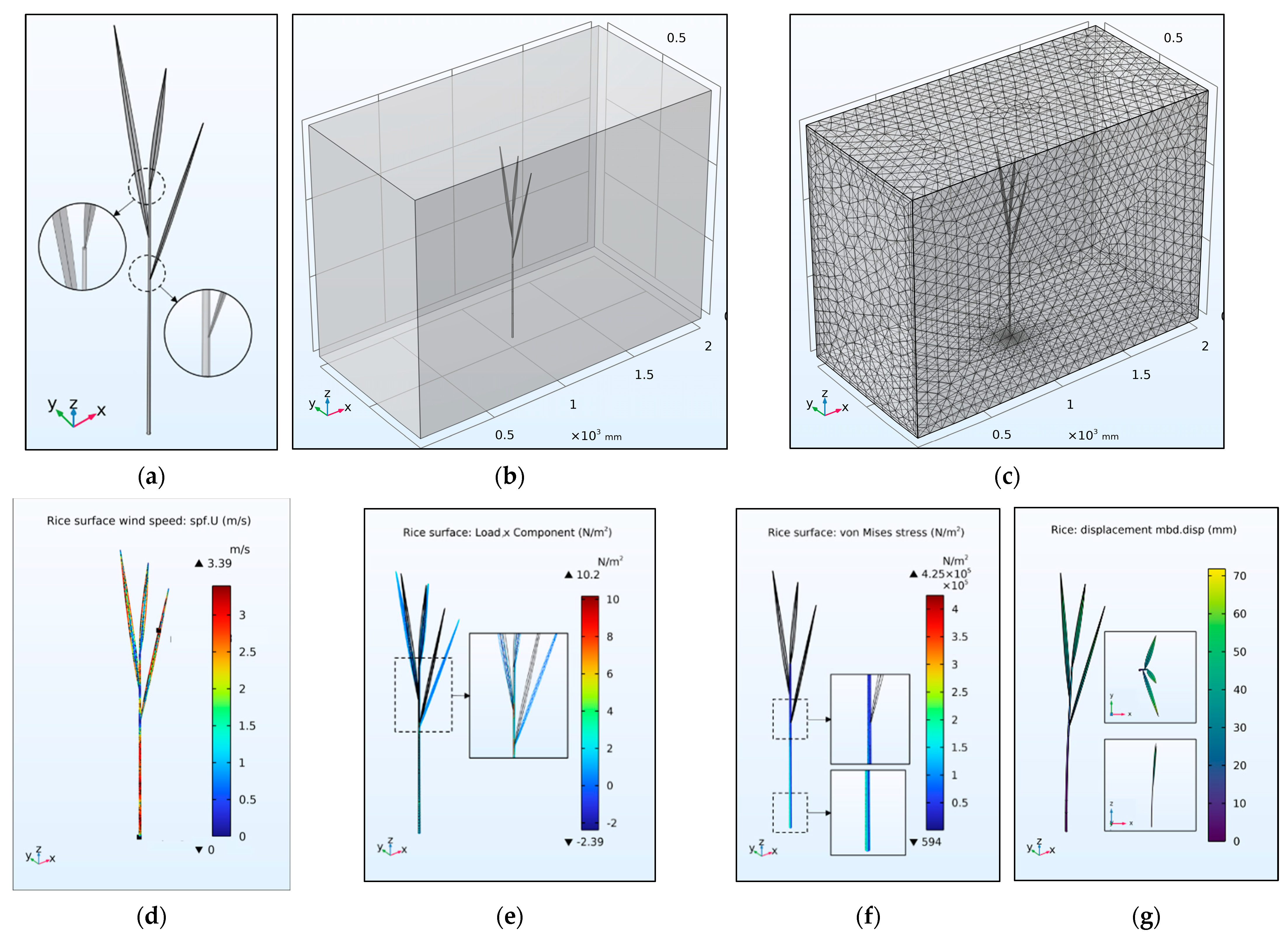
Before the finite element simulations, a simplified geometric model of single rice grains (choosing J1002 as an example) was parametrically modeled in COMSOL based on the data provided in Table 3, and different rice grains could be reconstructed by inputting new parameters (Figure 3a). A rectangle (2.0 m × 1.0 m × 1.5 m) was added as the fluid domain (Figure 3b) at the periphery of the rice, and the material parameters were set according to Table 4.
The model only considers the local natural wind field interacting with the rice, and at this height the vertical coherence of the natural wind field can be ignored [25]. The physical field of the fluid domain was selected as horizontal (o→x) laminar flow, using the velocity inlet and pressure outlet as the boundary conditions, in which the inlet was set to input the wind speed magnitude and the outlet was set considering zero static pressure and backflow suppression and the wind direction [26]. The solid domain physical field involved multibody dynamics, thereby defining rice as an orthotropic anisotropic material, adding gravity to rice by forming a fixed constraint between the bottom culm surface and the fluid domain. Each joint was fixed. The two physical fields were coupled via a fluid–solid coupling module to transfer the fluid loads to the solid structure, considering the inertial terms and geometric non-linearities.
Finally, we meshed the model with a tetrahedral grid and optimized the mesh by automatically correcting for distortion, thereby avoiding the generation of very small or inverted bending units. The number of boundary layers could be adjusted based on the geometry from three to five, finally generating a total of over 600,000 domain units (Figure 3c).
The model can be solved in the following two steps: (1) the wind speed at the surface of rice is analyzed under different wind fields (Figure 3d), and the corresponding wind pressure can be expressed as Equation (5), where is the wind resistance factor, set to 1.2 for slender cylinders [18]; (2) the wind load (Equation (6)) is applied to the rice surface using a boundary load (Figure 3e), and the corresponding von Mises equivalent stress (Figure 3f) and deformation of the rice structure (Figure 3g) can be calculated, where is the windward area in m2. Through iterations of the above two steps, the rice responses under different wind speeds can be obtained.
2.4. Wind-Induced Response Calculation and Validation
2.4.1. Rice Displacement under Different Wind Speeds
To verify the effectiveness of this model in simulating the displacement of rice in response to wind, in this section, the measured displacement changes of J1002 within a specific wind field are compared to the simulated values under the same conditions. As shown in Figure 4, three single rice grains were affixed onto an aluminum profile on the ground. The specific wind field was provided by electronically controlled fans (LY-30, Tianjin Lingyi Feiyang Technology Co., Tianjin, China), and a hot wire anemometer (KA33, Kanomax Co., Shenyang, China) was used to measure the inlet wind speed. A LiDAR sensor (3i-T1, 3iRobotix Co., Shenzhen, China) was installed at a height of 0.5 m to scan the displacement response of the sampled rice in real time, and a video camera (GoPro Hero 7, GoPro Inc., San Mateo, CA, USA) was adopted to record the entire test. The experiment was repeated three times, and the morphological data of the sampled rice were measured. Due to the rice leaves, the LiDAR sensor obtained the rice scatter at each moment. Here, we calculated the real-time x-directional displacement of rice via the k-means algorithm [27], considering the average of all scattered x-coordinates.
Accordingly, the rice geometry parameters, as well as the material properties in the RWRM, were modified based on the experimental setup. The inlet wind speed sequence was defined via an interpolation function according to the obtained hot wire anemometer data. The average displacement of rice at the 0.5 m height in this setting was calculated in the model with a time step consistent with the extraction interval of radar data frames.
2.4.2. Critical Wind Speed
To verify the effectiveness of this model in simulating the stress of the wind-induced response of the rice, in this section we use the acquired CWS data of the four rice varieties and compare the crop-specific CWS results of this model to those of existing solved models.
The rice culm is the structure that carries rice ears and transports nutrients. To prevent culm bending and breaking due to wind, the wind speed in the rice cultivation environment should be maintained below the CWS. In this study, the yield stress (, MPa) at 20% of the height of the main stem was used as the failure strength. The wind speed in the fluid domain was continuously adjusted so that the von Mises equivalent force approached the yield strength, and when the two values matched, the maximum wind speed at the rice culm surface was adopted as the CWS.
The yield strength obtained via the three-point bending test in Section 2.2.2 can be calculated as:
Here, is the breaking force in N; is the inertia of rotation in m4, which can be obtained with Equation (8):
To evaluate the model solution accuracy for the CWS, the calculation results were compared to those of the generalized crop lodging model [19]. The latter model can be expressed as Equation (9):
In the above equation, is a dimensionless parameter satisfying Equation (10); is the height of the center of gravity of the canopy, i.e., the culm length plus 1/3 of the spike length in m; and and refer to Table 4.
Here, is the circular frequency, rad/s, which satisfies Equation (11):
The remaining additional variables include the culm radius in mm; the calculated culm height in m; the culm number in dimensionless; the turbulence intensity in m, with [18]; and the damping ratio , with [28]. The maximum wind speed corresponding to each height of the rice culm was chosen as the CWS for the GLM via Equation (12):
3. Result
3.1. Wind-Induced Kinematic Response of Rice
The variation in the displacement of the x-component of rice at the number 2 position during the three repeated trials is shown in Figure 5. Figure 6 shows the wind speed data recorded by the hot wire anemometer. The results of the paired tests for the three sets of curves are shown, with the main wind speeds ranging from 2 to 5 m/s and considering mean inlet wind speeds of 3.2, 3.9, and 3.6 m/s.
The simulated and measured curves exhibited similar undulations, with the two curves being the most similar during the first repeated trial, while the largest difference occurred in the third trial. The more notable fluctuations in the measured data were mainly related to differences in the wind field, which were not strictly laminar in the field tests, and a certain amount of turbulence caused the rice displacement to sharply fluctuate. Hence, the simulation results were more sensitive to wind speed changes than the measured displacement curves. The various sets of curves showed a similar fluctuation range (Table 5), with a mean paired difference of 13.48 and mean error of 42.46 mm. The simulated and measured values were significant at the 1% level. Based on paired T-tests, there is a significant difference between the simulation and measurement results of the last two tests, yet the magnitude of the difference is relatively small (Cohen’s d was between 0.2 to 0.5). Combining the measured height at 0.5 m and response displacement of rice plants, the offset angle of rice culm can be calculated. An angle smaller than 45 degrees is beneficial in preventing lodging. The RWRM model could predict the amplitude of the wind-induced rice displacement at the 5 cm error level.
3.2. Critical Wind Speeds of Four Different Rice Species
When the equivalent force at 0.2 L exceeds the yield stress, the culm is considered to have failed, at which point the maximum wind speed at the culm surface can be selected as the CWS, with yield stresses of 2.00, 2.48, 2.14, and 1.91 MPa at 0.2 L for the four species.
The CWS values of the main stems were determined for each species, and corresponding theoretical CWS values were obtained with Equation (12). The average CWS value of the four rice species was 3.57 m/s, with NJ obtaining the largest value (4.37 m/s) and J1002 obtaining the smallest value (2.39 m/s), and the coefficient of variation indicated that there was little variability in the CWS values among the individual species. As previously mentioned, the maximum and average field wind speeds in South China during the rice-growing season are approximately 4.40 and 1.54 m/s, respectively, being generally lower than 3.30 m/s. Therefore, most rice clusters can resist natural winds during most of the growing period in the region.
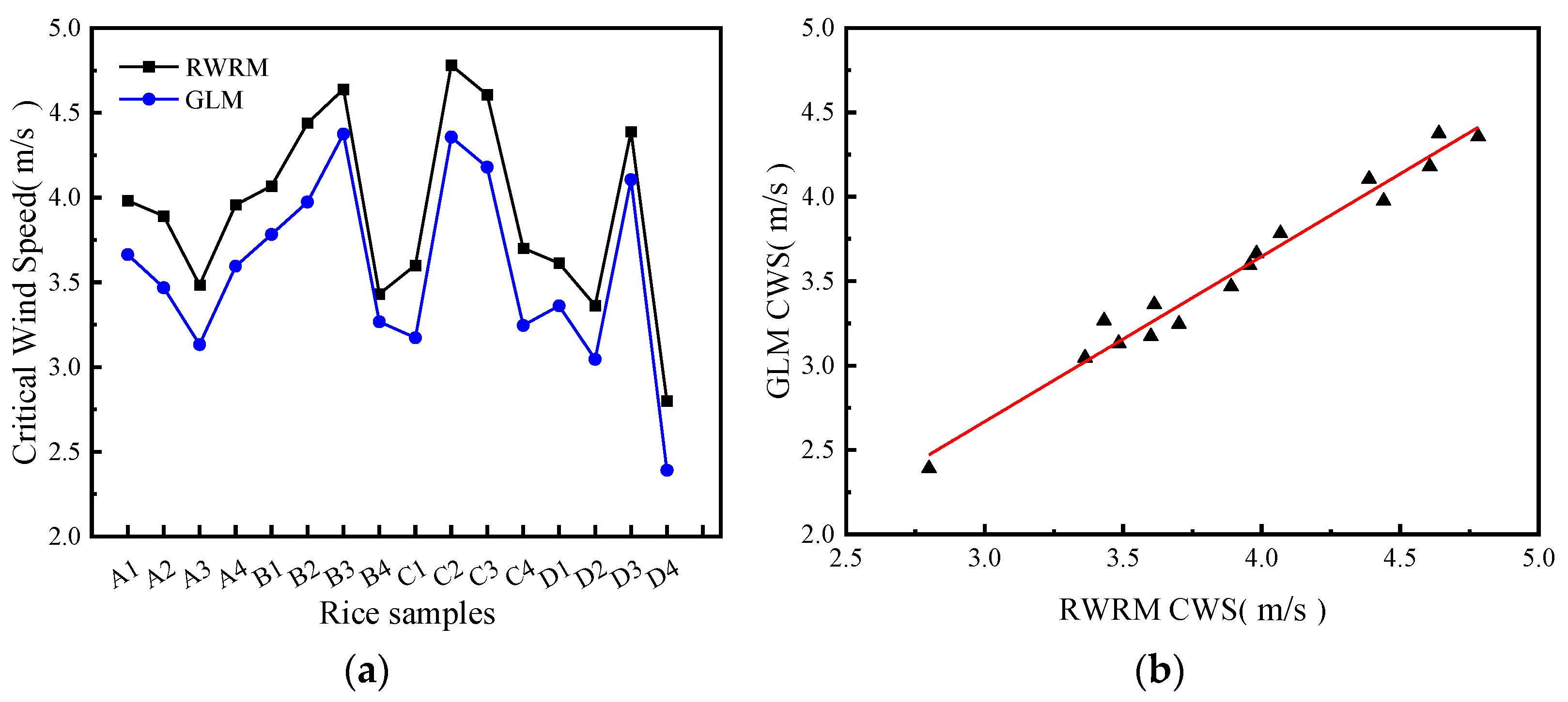
In Figure 7a, the simulated CWS is 3.938 ± 0.525 m/s and the theoretical CWS is 3.570 ± 0.542 m/s. The fold lines show that the CWS values of the RWRM differ from those of the GLM by 0.368 on average, and the RWRM achieved a wider CWS prediction range. This was mainly caused by the difference in the way the eigenfrequencies were calculated. The calculation results of the two models corresponded accordingly and could be linearly fitted (Figure 7b). The closer the slope of the straight line to 1, the more compatible the two models. The fit indicated a slope of 0.979 and a fitted R-squared value of 0.973. The RWRM results were highly similar to the GLM results, and the model obtained satisfactory accuracy in simulating the structural stress in the rice and predicting the CWS.
4. Discussion
The morphological and physical properties affect the rice response as well as the rice yield (the estimated thousand grain weight and final yield values first mentioned in Section 2.2.1 are listed in Table 6). The morphological indicators include the culm length , culm wall thickness , leaf area , and leaf angle (please refer to Table 2), and the physical properties include the Young’s modulus (please refer to Table 4), bending energy , culm moisture content , and leaf moisture content (please refer to Table 6), where the bending energy is the capacity of the rice culm to withstand bending deformation.
In this study, we used a grey correlation analysis to evaluate the degree of association between the above indicators and rice performance. The grey correlation analysis is a method used to quantitatively describe and compare the developmental changes in a system [29]. The concerned morphological and physical indicators were input as evaluation items, and the specific response indicators or yields were selected as correlation objects. In the analysis process, the degree of correlation between the evaluation items and correlation objects was obtained, and each evaluation item was ranked according to the magnitude of the correlation. The results are listed in Table 7. The correlation values ranged from 0 to 1. The correlation value approaches 1 when the correlation between the evaluation items and correlated objects is high.
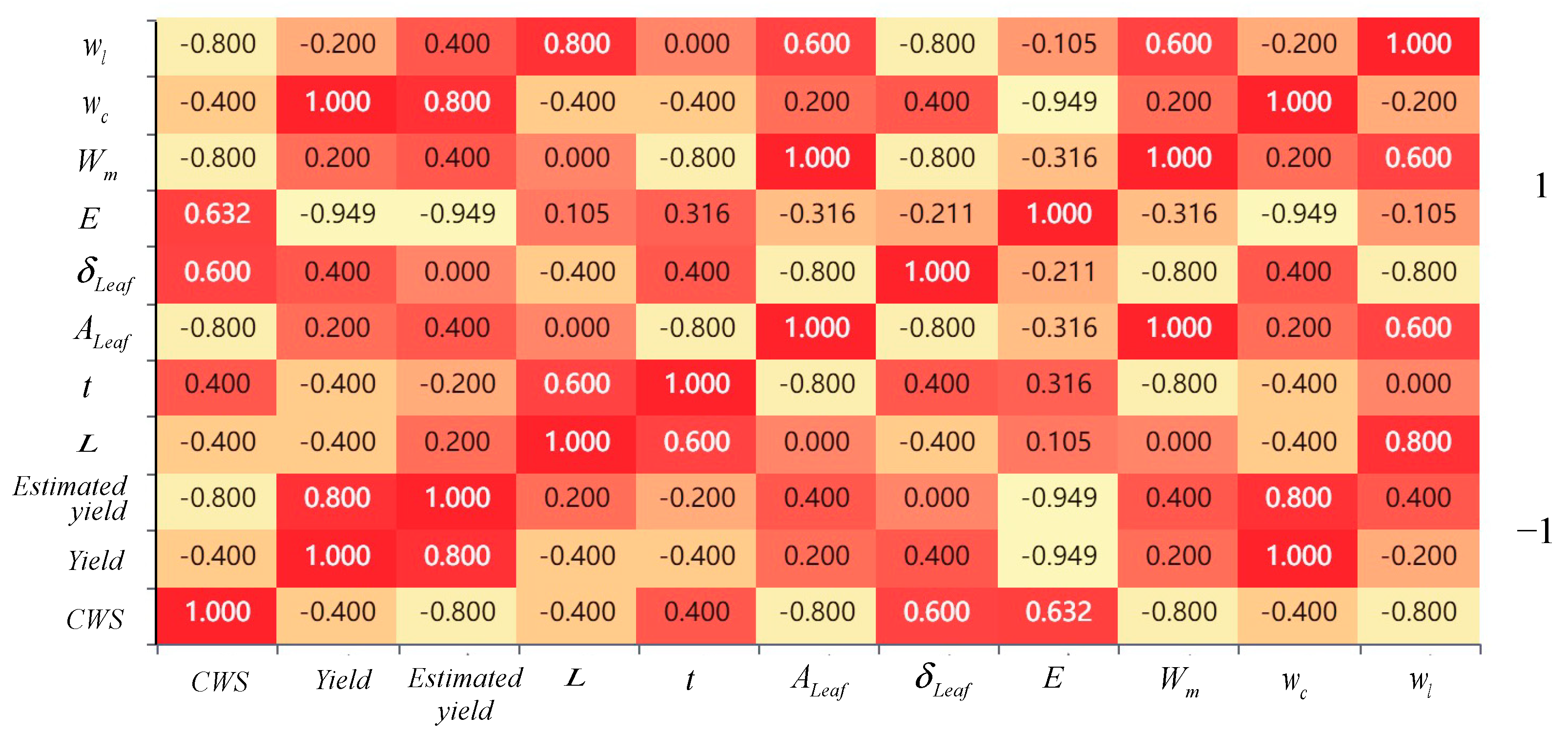
According to Table 7, the strength of the rice response was mainly determined by the Young’s modulus, culm wall thickness and size, moisture content, and culm length. The correlations between these variables were all higher than 0.8. The wind response of the rice was more notably influenced by its physical properties and culm size but depended less on the leaf characteristics. Conversely, the final yield was closely related to the leaf area and moisture content. The main correlations of the estimated yield did not follow the same trend as that of the final yield. In particular, the final yield exhibited a correlation of 0.919 with the estimated yield and 0.721 with the CWS. Pearson’s correlation analysis was conducted on the above indicators, and the heatmap is shown in Figure 8, with the results including correlation coefficients and significant p values.
The CWS was significantly negatively correlated with the leaf area and bending energy at the 5% level. The greater the leaf area and bending energy were, the lower the CWS. In addition, the longer the stalk and the higher the plant water content, the lower the CWS was, which increased the CWS that could reduce the rice yield to a certain extent, as an increase in the wind-induced response intensity requires a reduction in the leaf area, plant water content, or stalk length, while the leaf area was highly correlated with the yield, so the choice of reducing the plant height to increase the wind response intensity is preferred.
The rice yield was negatively correlated with the CWS, and there existed a strong correlation with the CWS. A relatively low CWS and high overall stability of rice were conducive to higher yields, while a decrease in Young’s modulus suggests an increase in the elasticity of the rice tissue structure. This occurs because dense rice leaves increase the strength of the wind-induced response of the rice and reduce the CWS of the rice, but due to favorable photosynthesis conditions, this situation promotes increased rice yields.
5. Conclusions
In this study, a finite element model for simulating the wind-induced motion response of rice was proposed. We calculated the wind-induced displacement and strength of rice stalks to obtain two important indicators of wind resistance in rice, namely the offset angle and critical wind speed, based on four rice species, i.e., 19X, NJ, T1002, and J1002. Furthermore, we discussed the impact of the rice’s wind resistance on the yield. The specific conclusions are summarized as follows:
- (1)
- The model could suitably predict the displacement range of rice in response to a horizontal wind field, with an average paired difference of 13.48 mm and an error value 42.46 mm, which means the model can predict the windward tilt angle of rice, with an average error of 5 degrees. This is beneficial for visually understanding the wind resistance of rice. A significant correlation at the 1% level between the simulated and measured displacements in the same time step helps to underpin the validity of the model;
- (2)
- The model could suitably predict the stress of rice, as evaluated via the CWS. The CWS of the four rice species was 3.57 m/s and its pairwise difference between this model and another existing high-impact model was 0.368 m/s on average. We found that the CWS is primarily affected by the condition of the rice culm, especially the Young’s modulus of the culm. The more robust the culm, the higher the CWS. The CWS is secondarily affected by rice leaves. The larger and heavier the rice leaves, the lower the CWS;
- (3)
- The rice’s yield has a negative correlation with its wind resistance. Larger and heavier rice leaves along with a lower Young’s modulus are instead conducive to increased rice yields. Both the displacement and CWS were mainly influenced by the physical properties, such as the Young’s modulus. A bigger displacement and lower CWS could result in a higher rice yield.
From a practical perspective, it is advisable to prevent rice plants from experiencing prolonged angular deviation and prolonged exposure to wind speeds that exceed the CWS limit of the species, while ensuring good crop yields. This is exactly what the data in this model support.
Author Contributions
Conceptualization, J.L. and X.H.; methodology, J.L., X.H. and H.L.; software, X.H.; validation, J.L., X.H. and H.L.; formal analysis, X.H.; investigation, X.H., H.L., H.W., B.L. and Z.L.; resources, X.H., H.L., H.W., B.L. and X.W.; data curation, J.L., X.H. and H.L.; writing—original draft preparation, X.H.; writing—review and editing, J.L. and X.H.; visualization, X.H.; supervision, J.L.; project administration, X.H.; funding acquisition, J.L. All authors have read and agreed to the published version of the manuscript.
Funding
This research was funded by Guangzhou Municipal Science and Technology Project, grant number 202206010164; and the Basic and Applied Basic Research Foundation of Guangdong Province, grant number 2023A1515011932.
Data Availability Statement
The data presented in this study are available on request from the corresponding author. The data are not publicly available due to the model will be further iterated, involved in the calculation of other parameters.
Conflicts of Interest
The authors declare no conflict of interest.
References
- Crops and Livestock Products. Available online: https://www.fao.org/faostat/en/#data/QCL/visualize (accessed on 26 February 2022).
- Muthayya, S.; Sugimoto, J.D.; Montgomery, S.; Maberly, G.F. An Overview of Global Rice Production, Supply, Trade, and Consumption. Ann. N. Y. Acad. Sci. 2014, 1324, 7–14. [Google Scholar] [CrossRef] [PubMed]
- Langre, E. Effects of Wind on Plants. Annu. Rev. Fluid Mech. 2008, 40, 141–168. [Google Scholar] [CrossRef]
- Gardiner, B.; Berry, P.; Moulia, B. Review: Wind Impacts on Plant Growth, Mechanics and Damage. Plant Sci. 2016, 245, 94–118. [Google Scholar] [CrossRef] [PubMed]
- Luo, X.; Wu, Z.; Fu, L.; Dan, Z.; Yuan, Z.; Liang, T.; Zhu, R.; Hu, Z.; Wu, X. Evaluation of Lodging Resistance in Rice Based on an Optimized Parameter from Lodging Index. Crop Sci. 2022, 62, 1318–1332. [Google Scholar] [CrossRef]
- Shah, L.; Yahya, M.; Shah, S.M.A.; Nadeem, M.; Ali, A.; Ali, A.; Wang, J.; Riaz, M.W.; Rehman, S.; Wu, W.; et al. Improving Lodging Resistance: Using Wheat and Rice as Classical Examples. Int. J. Mol. Sci. 2019, 20, 4211. [Google Scholar] [CrossRef]
- Klerkx, L.; Jakku, E.; Labarthe, P. A Review of Social Science on Digital Agriculture, Smart Farming and Agriculture 4.0: New Contributions and a Future Research Agenda. NJAS-Wagening. J. Life Sci. 2019, 90, 100315. [Google Scholar] [CrossRef]
- Radoglou-Grammatikis, P.; Sarigiannidis, P.; Lagkas, T.; Moscholios, I. A Compilation of UAV Applications for Precision Agriculture. Comput. Netw. 2020, 172, 107148. [Google Scholar] [CrossRef]
- Guo, S.; Li, J.; Yao, W.; Zhan, Y.; Li, Y.; Shi, Y. Distribution Characteristics on Droplet Deposition of Wind Field Vortex Formed by Multi-Rotor UAV. PLoS ONE 2019, 14, e0220024. [Google Scholar] [CrossRef]
- Finnigan, J. Turbulence in Waving Wheat: I. Mean Statistics and Honami. Bound. -Layer Meteorol. 1979, 16, 181–211. [Google Scholar] [CrossRef]
- Doaré, O.; Moulia, B.; Langre, E. Effect of Plant Interaction on Wind-Induced Crop Motion. J. Biomech. Eng. 2004, 126, 146–151. [Google Scholar] [CrossRef]
- Py, C.; Langre, E.; Moulia, B.; Hémon, P. Measurement of Wind-Induced Motion of Crop Canopies from Digital Video Images. Agric. For. Meteorol. 2005, 130, 223–236. [Google Scholar] [CrossRef]
- Joseph, G.; Mohammadi, M.; Sterling, M.; Baker, C.; Gillmeier, S.; Soper, D.; Jesson, M.; Blackburn, G.A.; Whyatt, J.D.; Gullick, D.; et al. Determination of Crop Dynamic and Aerodynamic Parameters for Lodging Prediction. J. Wind Eng. Ind. Aerodyn. 2020, 202, 104169. [Google Scholar] [CrossRef]
- Dupont, S.; Gosselin, F.; Py, C.; Langre, E.; Hemon, P.; Brunet, Y. Modelling Waving Crops Using Large-Eddy Simulation: Comparison with Experiments and a Linear Stability Analysis. J. Fluid Mech. 2010, 652, 5–44. [Google Scholar] [CrossRef]
- Yang, X.-S. Introduction to Computational Mathematics, 2nd ed.; World Scientific: Singapore, 2015; ISBN 978-981-4635-77-6. [Google Scholar]
- Yang, M.; Défossez, P.; Danjon, F.; Fourcaud, T. Tree Stability under Wind: Simulating Uprooting with Root Breakage Using a Finite Element Method. Ann. Bot. 2014, 114, 695–709. [Google Scholar] [CrossRef] [PubMed]
- Baker, C. The Development of a Theoretical Model for the Windthrow of Plants. J. Theor. Biol. 1995, 175, 355–372. [Google Scholar] [CrossRef]
- Berry, P.; Sterling, M.; Baker, C.; Spink, J.; Sparkes, D. A Calibrated Model of Wheat Lodging Compared with Field Measurements. Agric. For. Meteorol. 2003, 119, 167–180. [Google Scholar] [CrossRef]
- Baker, C.; Sterling, M.; Berry, P. A Generalised Model of Crop Lodging. J. Theor. Biol. 2014, 363, 1–12. [Google Scholar] [CrossRef]
- Wang, N.; Wang, F.; Shock, C.; Meng, C.; Huang, Z.; Gao, L.; Zhao, J. Evaluating Quinoa Stem Lodging Susceptibility by a Mathematical Model and the Finite Element Method under Different Agronomic Practices. Field Crop. Res. 2021, 271, 108241. [Google Scholar] [CrossRef]
- Fariñas, M.D.; Sancho-Knapik, D.; Peguero-Pina, J.; Gil-Pelegrín, E.; Gómez Álvarez-Arenas, T. Shear Waves in Vegetal Tissues at Ultrasonic Frequencies. Appl. Phys. Lett. 2013, 102, 103702. [Google Scholar] [CrossRef]
- Liu, G.; Ghosh, R.; Vaziri, A.; Hossieni, A.; Mousanezhad, D.; Nayeb-Hashemi, H. Biomimetic Composites Inspired by Venous Leaf. J. Compos. Mater. 2018, 52, 361–372. [Google Scholar] [CrossRef]
- Stubbs, C.J.; Oduntan, Y.A.; Keep, T.R.; Noble, S.D.; Robertson, D.J. The Effect of Plant Weight on Estimations of Stalk Lodging Resistance. Plant Methods 2020, 16, 128. [Google Scholar] [CrossRef] [PubMed]
- Zhou, F.; Huang, J.; Liu, W.; Deng, T.; Jia, Z. Multiscale Simulation of Elastic Modulus of Rice Stem. Biosyst. Eng. 2019, 187, 96–113. [Google Scholar] [CrossRef]
- Cheynet, E. Influence of the Measurement Height on the Vertical Coherence of Natural Wind. In Proceedings of the XV Conference of the Italian Association for Wind Engineering; Ricciardelli, F., Avossa, A.M., Eds.; Lecture Notes in Civil Engineering; Springer International Publishing: Cham, Switzerland, 2019; Volume 27, pp. 207–221. ISBN 978-3-030-12814-2. [Google Scholar]
- Liu, M.; Liao, H.; Li, M.; Ma, C.; Yu, M. Long-Term Field Measurement and Analysis of the Natural Wind Characteristics at the Site of Xi-Hou-Men Bridge. J. Zhejiang Univ. Sci. A 2012, 13, 197–207. [Google Scholar] [CrossRef]
- Hartigan, J.; Wong, M. Algorithm AS 136: A K-Means Clustering Algorithm. J. R. Stat. Soc. Ser. C Appl. Stat. 1979, 28, 100–108. [Google Scholar] [CrossRef]
- Finnigan, J. Turbulence in Plant Canopies. Annu. Rev. Fluid Mech. 2000, 32, 519–571. [Google Scholar] [CrossRef]
- Xu, J.; Liu, Z.; Yin, L.; Liu, Y.; Tian, J.; Gu, Y.; Zheng, W.; Yang, B.; Liu, S. Grey Correlation Analysis of Haze Impact Factor PM2.5. Atmosphere 2021, 12, 1513. [Google Scholar] [CrossRef]
Figure 1.
Types of rice lodging: (a) caused by natural wind; (b) caused by an agricultural drone.

Figure 2.
(a) Rice sample one week after tassel (the red marks ①②③ are the intercepted parts of the mechanical test specimens corresponding in Table 3). (b) WE-D series precision micro-controlled electronic universal testing machine, for conducting tensile and bending tests.
Figure 2.
(a) Rice sample one week after tassel (the red marks ①②③ are the intercepted parts of the mechanical test specimens corresponding in Table 3). (b) WE-D series precision micro-controlled electronic universal testing machine, for conducting tensile and bending tests.

Figure 3.
Model setup and calculation process: (a) geometric model of single rice plant; (b) fluid domains in the rice plant’s periphery; (c) mesh; (d) wind speed at the near point of the rice surface when the inlet wind speed was set as 4 m/s; (e) boundary loads on rice under this wind field; (f) von Mises equivalent stress of rice; (g) a change in the posture of the rice.

Figure 4.
Test layout. The number 1, 2 and 3 are used to indicate specific positions of tested rice.
Figure 4.
Test layout. The number 1, 2 and 3 are used to indicate specific positions of tested rice.

Figure 5.
The simulated and measured displacements (x-component) of rice culm at the height of 0.5 m at different inlet wind speeds in Figure 6. (a) mean inlet wind speeds of 3.2 m/s; (b) mean inlet wind speeds of 3.9 m/s; (c) mean inlet wind speeds of 3.6 m/s.
Figure 5.
The simulated and measured displacements (x-component) of rice culm at the height of 0.5 m at different inlet wind speeds in Figure 6. (a) mean inlet wind speeds of 3.2 m/s; (b) mean inlet wind speeds of 3.9 m/s; (c) mean inlet wind speeds of 3.6 m/s.

Figure 6.
Wind speed measured by the hot wire anemometer during three repeated tests.

Figure 7.
(a) Critical wind speeds for the main stems of each species under both models. The letter A stands for 19X, B for NJ, C for T1002, and D for J1002. (b) FEM with GLM linear fit, where the equation is y = −0.268 (±0.166) + 0.979 (±0.042)x, with a Pearson’s r value of 0.987, R square of 0.975, and adjusted R square of 0.973.

Figure 8.
Heat map of correlation coefficients for Pearson’s correlation analysis of rice indicators.
Figure 8.
Heat map of correlation coefficients for Pearson’s correlation analysis of rice indicators.


Table 1.
Varieties of rice tested and the growth period.
| Species Name * | Abbr. | Rice Type | Rice Growth Period (Date of 2021) | |||
|---|---|---|---|---|---|---|
| Sowing | Tassel | Spike | Harvest | |||
| 19 Xiang | 19X | Conventional indica | 16 July | 28 September | 1 October | 3 November |
| Nan Jing Xiang Zhan | NJ | 16 July | 26 September | 29 September | 3 November | |
| Taiyou 1002 | T1002 | Triple hybrid indica | 11 July | 25 September | 28 September | 3 November |
| Jifengyou 1002 | J1002 | 11 July | 30 September | 4 October | 3 November | |
* All four rice species are late-season rice and the breeding information is detailed in the China Rice Data Center: https://www.ricedata.cn/ (accessed on 20 March 2023).
Table 2.
Rice agronomic characteristics.
| Species * | /mm | /mm | /mm | /mm | /mm | /mm | /deg |
|---|---|---|---|---|---|---|---|
| 19X | 1155.0 | 896.3 | 9.68 | 2.07 | 520.7 | 15.8 | 10.00 |
| NJ | 1063.8 | 790.0 | 8.69 | 1.92 | 523.6 | 13.1 | 23.25 |
| T1002 | 1135.0 | 851.3 | 9.81 | 1.81 | 504.2 | 13.6 | 31.08 |
| J1002 | 1057.5 | 825.5 | 8.39 | 1.35 | 530.1 | 16.7 | 11.50 |
* The average spike weight and length for this period were 3.66 g and 26.46 cm, respectively. Due to the lighter spike weight, rice spike characteristics were not considered in the finite element model.
Table 3.
Mechanical test settings.
| Test Type | Rice Part * | Four Species’ Average Specimen Cross-Sectional Areas (mm2) | Gauge Length (mm) | Loading Speed (mm/min) |
|---|---|---|---|---|
| Uniaxial tensile | The 1st leaf | 4.98/3.65/3.77/5.28 | 60 | 2 |
| The 2nd leaf | 3.99/2.87/3.05/4.25 | 60 | 2 | |
| Culm | 8.00/9.34/10.38/14.67 | 30 | 20 | |
| Three-point bending | Culm | 30.06/31.93/25.98/39.97 | 70 | 20 |
* The exact rice parts of the interception can be referred in Figure 2a (marked in red), which the 1st leaf was the part ①, the 2nd leaf was the part ② and the culm was the part ③).
Table 4.
Main material properties of RWRM.
| Properties * | Variables | Species | Parts | Value | Source |
|---|---|---|---|---|---|
| Young’s modulus | (GPa) | 19X | culm | 0.63 | Measured/calculated |
| leaf | 0.72/0.60 | Measured/calculated | |||
| NJ | culm | 0.63 | Measured/calculated | ||
| leaf | 0.31/0.38 | Measured/calculated | |||
| T1002 | culm | 0.59 | Measured/calculated | ||
| leaf | 0.66/0.72 | Measured/calculated | |||
| J1002 | culm | 0.56 | Measured/calculated | ||
| leaf | 0.54/0.61 | Measured/calculated | |||
| Density | (kg/m3) | All | culm | 1046 | Measured/calculated |
| leaf | 1026 | Measured/calculated | |||
| Poisson’s ratio | (dimensionless) | All | culm | 0.30 | Referred [21,22] |
| leaf | 0.28 | Referred [23,24] | |||
| Air density | (kg/m3) | / | / | 1.18 | COMSOL built-in material library |
| Aerodynamic viscosity | (Pa·s) | / | / | 1.84 × 10⁻⁵ | COMSOL built-in material library |
| Gravity acceleration | (m/s2) | / | / | 9.78 | Constant |
* The same set of material parameters is used for culms and leaf veins and the 2nd and 3rd leaves. The air density and dynamic viscosity are taken as the corresponding values at 1 atm and 298.15 K, respectively.
Table 5.
Statistical description of rice wind response results of three repeated experiments.
| Parameter | 1 | 2 | 3 | |||
|---|---|---|---|---|---|---|
| RWRM | Measured | RWRM | Measured | RWRM | Measured | |
| Quantity | 87 | 87 | 87 | 87 | 87 | 87 |
| Maximum(mm) | 179.51 | 190.75 | 181.10 | 199.29 | 122.41 | 227.76 |
| Minimum(mm) | 0.06 | −2.85 | 0 | −5.69 | 0.07 | −2.85 |
| Average(mm) | 76.80 | 74.19 | 75.71 | 56.05 | 52.37 | 70.55 |
| Paired Difference(mm) | 2.61 | 19.66 | −18.17 | |||
| Paired t-tests p 1 | 0.595 | 0.003 *** | 0.006 *** | |||
| Cohen’s d | 0.058 | 0.330 | 0.303 | |||
| Pearson’s p 1 | 0.480 *** | 0.560 *** | 0.321 *** | |||
1 p is the correlation coefficient, and *** means the concerning values were significant at the 1% level.
Table 6.
Potential factors influencing wind resistance performance in rice.
| Species | Estimated Thousand Grain Weight (g) | Final Yield (g/50 Plants) | Bending Energy (mJ) | Culm Moisture Content (%) | Leaf Moisture Content (%) |
|---|---|---|---|---|---|
| 19X | 21.4 | 1586.37 | 178.86 | 85.90 | 73.07 |
| NJ | 21.7 | 1547.70 | 146.27 | 86.39 | 67.16 |
| T1002 | 23.5 | 1648.43 | 132.45 | 87.02 | 70.12 |
| J1002 | 26.5 | 2070.93 | 247.04 | 87.31 | 71.11 |
Table 7.
Results of the grey correlation analysis.
| Indicators | CWS | Final Yield | Estimated Yield | |
|---|---|---|---|---|
| Morphology | 0.800 (4) | 0.798 (4) | 0.873 (3) | |
| 0.871 (2) | 0.748 (6) | 0.772 (5) | ||
| 0.660 (6) | 0.867 (1) | 0.821 (4) | ||
| 0.502 (8) | 0.431 (8) | 0.421 (8) | ||
| Physical properties | 0.879 (1) | 0.763 (5) | 0.747 (6) | |
| 0.591 (7) | 0.743 (7) | 0.660 (7) | ||
| 0.856 (3) | 0.813 (3) | 0.841 (1) | ||
| 0.797 (5) | 0.818 (2) | 0.840 (2) | ||
Note: The data format is “correlation value (rank order by value size)”. The resolution factor is 0.5.
Disclaimer/Publisher’s Note: The statements, opinions and data contained in all publications are solely those of the individual author(s) and contributor(s) and not of MDPI and/or the editor(s). MDPI and/or the editor(s) disclaim responsibility for any injury to people or property resulting from any ideas, methods, instructions or products referred to in the content. |
© 2023 by the authors. Licensee MDPI, Basel, Switzerland. This article is an open access article distributed under the terms and conditions of the Creative Commons Attribution (CC BY) license (https://creativecommons.org/licenses/by/4.0/).
Share and Cite
MDPI and ACS Style
Hu, X.; Li, H.; Wu, H.; Long, B.; Liu, Z.; Wei, X.; Li, J. Modeling the Kinematic Response of Rice under Near-Ground Wind Fields Using the Finite Element Method. Agronomy 2023, 13, 1178. https://doi.org/10.3390/agronomy13041178
AMA Style
Hu X, Li H, Wu H, Long B, Liu Z, Wei X, Li J. Modeling the Kinematic Response of Rice under Near-Ground Wind Fields Using the Finite Element Method. Agronomy. 2023; 13(4):1178. https://doi.org/10.3390/agronomy13041178
Chicago/Turabian StyleHu, Xiaodan, Huifen Li, Han Wu, Bo Long, Zhijie Liu, Xu Wei, and Jiyu Li. 2023. "Modeling the Kinematic Response of Rice under Near-Ground Wind Fields Using the Finite Element Method" Agronomy 13, no. 4: 1178. https://doi.org/10.3390/agronomy13041178
Note that from the first issue of 2016, this journal uses article numbers instead of page numbers. See further details here.