Selection of a Navigation Strategy According to Agricultural Scenarios and Sensor Data Integrity

Abstract

In digital farming, the use of technology to increase agricultural production through automated tasks has recently integrated the development of AgBots for more reliable data collection using autonomous navigation. These AgBots are equipped with various sensors such as GNSS, cameras, and LiDAR, but these sensors can be prone to limitations such as low accuracy for under-canopy navigation with GNSS, sensitivity to outdoor lighting and platform vibration with cameras, and LiDAR occlusion issues. In order to address these limitations and ensure robust autonomous navigation, this paper presents a sensor selection methodology based on the identification of environmental conditions using sensor data. Through the extraction of features from GNSS, images, and point clouds, we are able to determine the feasibility of using each sensor and create a selection vector indicating its viability. Our results demonstrate that the proposed methodology effectively selects between the use of cameras or LiDAR within crops and GNSS outside of crops, at least 87% of the time. The main problem found is that, in the transition from inside to outside and from outside to inside the crop, GNSS features take 20 s to adapt. We compare a variety of classification algorithms in terms of performance and computational cost and the results show that our method has higher performance and lower computational cost. Overall, this methodology allows for the low-cost selection of the most suitable sensor for a given agricultural environment.

1. Introduction

With the increase in market competitiveness and food demand due to population growth and more demanding consumers with respect to product quality, farmers have been betting on the data-based decision-making processes to reduce operational failures [1]. In this way, data are required to be accurate and reliable, which is why numerous studies have been carried out whose objective is to use AgBots in agriculture [2].

There are several applications in which AgBots can be beneficial for agriculture, enabling the development of methods to optimize processes and generate fewer losses, such as irrigation [3,4] (optimizing water use) and weed identification [5,6] (reduction in plant losses due to diseases).

For the application of AgBots in the agricultural environment to be possible, navigation strategies are needed to allow them to move safely around the plantation [7]. According to [8,9], a robot can navigate in environments: (i) structured (when it is well defined) and (ii) unstructured (when it is not well defined). In the agricultural context, the environment is mostly unstructured and contains several types of obstacles. Due to these circumstances, it can be inferred that navigation for an AgBot, as well as for several mobile robots, is one of the main challenges in this field [10].

These challenges make many navigation strategies limit their solutions based on specific situations that AgBots may face. In general, navigation strategies for AgBots can be simplified into two types with respect to field crops: (i) outside crop, when the AgBot is out the crop and movement control methods are sufficient to ensure navigation; and (ii) inside crop, when the AgBot is inside the crop and it becomes necessary to identify patterns of crop behaviour to navigate [11,12,13].

In this context, the present work proposes the development of a methodology for selecting navigation strategies, relating data from different sensors (GNSS, LiDAR and camera) and the environment in which the robot navigates.

1.1. Related Works

According to [14,15], the main sensors used in AgBots are RGB cameras, GNSS, and LiDAR. Therefore, this work will address methods that carry out or propose navigation strategies using these sensors. It is important to note that such sensors may suffer from problems such as low accuracy in the GNSS data when there is a signal obstruction, LiDAR suffers from occlusions, and cameras have low tolerance to lighting changes.

In this context, Sigrist et al. [16] presented a study on the impact the plant canopy has on the quality of the GNSS signal. The authors showed that foliage is one of the biggest sources of error in signal reception, decreasing the efficiency of data acquisition by up to 47%. Furthermore, other studies have been conducted to analyse the impact that forests [17], plantations [18] and buildings [19] have on the GNSS signal. For this reason, the application of navigation strategies using GNSS in the agricultural scenario is carried out mainly outside of the cultivation or in low-lying crops. As an example, the work proposed by [20] used RTK-GNSS to navigate in a potato crop, which did not obstruct the sensor signal.

In agricultural environments, LiDAR sensors are widely used to identify crop phenotypes [21] and for under-canopy navigation [22]. In such scenarios, there are a few problematic situations that can compromise sensor data. Higuti et al. [23] identified the main types of interference based on the point cloud obtained by a LiDAR as (i) collisions, (ii) end of cropping, and (iii) cropping gaps. In [24], the authors proposed a semantic classification algorithm for LiDAR data based on the condition of the crop as a navigation aid strategy when building a topological map. In [25], a method was proposed to identify anomalies such as obstacles and collisions based on a LiDAR point cloud.

Cameras are also widely used for various applications in agriculture, including plantation segmentation [26], classification of crop species [27], and the development of AgBots navigation strategies [28]. However, the application of cameras in the agricultural environment suffers from occlusions and variations in luminosity [29,30]. Due to this, many studies have proposed lighting control for cameras in applications in this environment [31,32].

Different navigation strategies can be applied to AgBots; however, these systems, individually, do not guarantee complete autonomous navigation. In general, many studies have focused on navigation strategies for specific situations, which do not allow fully autonomous navigation in an agricultural environment.

In [33], there was a proposal for the fusion of information from different navigation strategies, using stereo vision, omnidirectional vision and GNSS. To achieve this objective, the author proposed the identification of navigable areas, obstacles, and faults. The proposed methodology works in layers: (i) data fusion to estimate AgBot attitude using GNSS, IMU and encoders; (ii) suggested control that indicates locations to which the platform can navigate based on the response of the vision systems; and (iii) list failures that indicate AgBot kinematic limitations.

In [34], the authors proposed a methodology in ROS for the autonomous navigation of a mobile robot. The methodology is composed of layers: sensors, pre-processing, and localization and mapping. From this information, a task manager makes a selection of the appropriate robot behaviour and sends the decision to the trajectory-planning system.

The work in [35] used GNSS, IMU, LiDAR, and a camera in a methodology for autonomous navigation in agricultural environments in order to avoid dynamic obstacles. When defining the waypoints, the system plans the AgBot trajectory and executes the movement control. At the same time, the local dynamic planner locates agents (obstacles) and estimates their movements using RNN. The exit condition is made by the high-level controller, which switches the systems based on the proximity of dynamic and static agents and waypoints.

1.2. Contributions

Few studies have focused on the development of methodologies that combine or select navigation strategies for agricultural environments. In general, previous work in this field may be limited to a proposal [34], or do not present experimental results [33] or use techniques that require high computational processing [35]. In this context, the main contribution of this research is the development of a methodology for selecting navigation strategies based on data from different sensors (GNSS, LiDAR and camera) and the environment in which the AgBot navigates. For this, we used different classification models and analysed the response time of the methodology. The results show that the methodology has an accuracy of at least 87% for selecting navigation strategies using GNSS outside the crop and navigation strategies using LiDAR or camera inside the crop or under-canopy, based on extensive data collected in a sugarcane crop.

2. Materials and Methods

An overview of the methodology proposed in this work is presented in Figure 1.

In this section, we describe the characteristics of the AgBot and present the experimental setup used for data collection in a sugarcane plantation, showing details of the cultivation and its importance for Brazil. Next, the predictor and predicted variables that are used in the classification techniques are discussed. Subsequently, how the fusion of information from the classifiers is carried out is presented.

2.1. AgBot

The AgBot used for data acquisition was the TerraSentia 2020 (TS2020) developed by EarthSense Inc. This robot has dimensions of 0.32 × 0.54 × 0.4 m${}^3$ (width, length, and height), it has a differential direction, and the main components of this platform can be seen in

Table 1. Components of AgBot TS2020.

AgBot *	Components	Characteristics
	Battery	14.8 V 10,000 mAh
	Motor	Maytech Brushless Outrunner Hub
	Computer	NUC-I7 Processor
	Operational System	Ubuntu 18.04
	LiDAR	UST-10LX
	IMU	Bosch BNO0555
	GNSS	Ublox Zed-F9P
	Camera	RGB cameras with LED Illumination

* Courtesy of EarthSense Inc.

.

2.2. Experimental Setup

The experiments were carried out in a sugarcane (Saccharum officinarium L.) field at the regrowth stage in a farm in Água Vermelha (Latitude: 21${}^{\circ }$53${}^{\prime }$48${}^{″}$ S, Longitude: 47${}^{\circ }$53${}^{\prime }$35${}^{″}$ W), district of São Carlos, located in São Paulo, Brazil.

This crop was selected because Brazil is the largest sugarcane producer in the world. According to data from [36], in 2020, Brazil produced approximately 45% of the world’s sugarcane. Furthermore, Brazil processes several by-products of sugarcane, such as biofuels and sugar, which have a strong impact on its economy [37].

2.3. Predicted and Predictors Variables

The predictor and predicted variables used for agricultural scenario classification were defined based on the sensor data used.

2.3.1. GNSS

We proposed investigating the behaviour of the GNSS sensor data in the three scenarios presented in

Table 2. Predicted environment using GNSS.

Representation	Class	Distance between Crops (m)
	GNSSOutsideCrop	≥3.00
	GNSSInsideCrop	≥1.00
	UnderCanopy	<1.00

. The first scenario was GNSSOutsideCrop which represents the ideal situation for navigation using GNSS, where the distance between the crops is greater or equal to 3.00 m. The second scenario was GNSSInsideCrop, which indicates that the platform is inside the crop, but there is no superior obstruction in the GNSS signal, only lateral obstruction, where the distance between the crops is greater or equal to 1.00 m. Finally, the third scenario was UnderCanopy, which indicates that the robot is inside the crop in a situation where there is lateral and superior obstruction for the GNSS signal, where the distance between the crops is less than 1.00 m.

The predictor variables selected for the analysis using GNSS are presented in

Table 3. Predictor variables using GNSS.

Feature	Variable Name	Unit
Heading Accuracy	HeadAcc	${}^{\circ }$
Horizontal Accuracy	HorAcc	m
Speed Accuracy	SpeedAcc	m/s

. As presented in the literature, obstruction of the GNSS signal causes a decrease in the accuracy presented by the GNSS measurements. Therefore, it was proposed to investigate the data provided by the AgBot TerraSentia in relation to heading, horizontal, and speed accuracy.

2.3.2. LiDAR

The variable classes based on the LiDAR point cloud are also related to the scenario in which the AgBot navigates and are presented in

Table 4. Predicted environment using LiDAR.

Representation	Class	Description
	LiDAROutsideCrop	There is no crop.
	LiDARInsideCrop	There is at least one row crop.
	LiDAROcclusion	Many points surrounding origin.

. The first class (LiDAROutsideCrop) represents the condition in which the robot is outside the crop. The second class (GNSSInsideCrop) represents the situation in which the platform is inside the crop, regardless of whether there are one or two crop lines. Furthermore, finally, the third class (LiDAROcclusion) indicates that the sensor is obstructed by some object, therefore it is unknown whether it is inside or outside the crop.

When analysing each of the classes in Table 4, different distributions of point cloud were noticed. For the LiDARInsideCrop condition, on the X-axis, when there were two crop lines, the distribution resembled a U-shape and when there was only one crop line, it resembled a J-shape. For the LiDAROutsideCrop the presence of high randomness was noted, both on the X- and Y-axis. Regarding the LiDAROcclusion class, a dense number of points close to the sensor was observed and they do not characterize a specific distribution. In addition, it was proposed to analyse whether the intensity of the return signal of the infrared beam can help in the identification of these classes, similarly to [38] that used laser intensity to identify defects in railway tunnel linings.

With this in mind, the X-, Y- and intensity-axes were characterized as random variables, as presented in [39]. To characterize the distribution of these variables, there are some parameters that can be used; in this work, the variables that were investigated are presented in

Table 5. Predictor variables using LiDAR.

Feature	Variable Name	Equation
Mean	${\mu }_{X,Y,I}$	$\frac{1}{k}{\sum }_{i=1}^k\left(x_i\right)$
Variance	${\sigma }_{X,Y,I}$	$\frac{1}{k}{\sum }_{i=1}^k{\left(x_i-\overline{x}\right)}^2$
Skewness	${\gamma }_{X,Y,I}$	$\frac{1}{k}{\sum }_{i=1}^k{\left(\frac{x_i-\overline{x}}{\sigma }\right)}^3$

.

2.3.3. RGB Camera

As discussed before, the camera suffers mainly from lighting problems and occlusions. Therefore, the classification algorithm for this sensor aimed to identify these limitations that make the use of data from this sensor unfeasible. Five classes that indicate the quality of the analysed image were classified, according to

Table 6. Predicted environment using Camera.

Representation	Class	Description
	Ideal	There is no problem in the image.
	HighBrightness	Image is too bright.
	LowBrightness	Image is too dark.
	Blur	Image loses details.
	CameraOcclusion	Camera is occluded.

.

The first class (Ideal) represents the condition in which the image does not have a problem. The second class (HighBrightness) indicates the situation in which there is a lot of incident light on the camera transducer. On the other hand, the third class (LowBrightness) symbolizes the opposite situation, in which there is not enough time to focus a lot of light on the camera transducer, resulting in a dark image. This scenario happens because inner-row distance changes can cause an increase or decrease in the amount of light that enters the environment and it takes time for the camera to adapt to the new light level. The fourth class (Blur) corresponds to the situation in which the camera does not have time to focus, resulting in a blurred image. Navigation through uneven soil can result in vibrations in the robot, which can affect the cameras leading to blurred images. Finally, the fifth class (CameraOcclusion) indicates that the camera is obstructed by leaves or branches.

Note that the classes differ with respect to the amount of light and sharpness or the presence of texture in the image; therefore, the selected characteristics must be sensitive to this. Based on this scenario, the image is converted from the RGB colourspace to the greyscale colourspace. In addition, to identify the lack of textures in the image, the Laplacian operator was used, which is an edge descriptor that can be particularly useful in identifying blurred images, where there are very few edges. The predictor variables for the camera are summarized in

Table 7. Predictor Variables using camera.

Feature	Variable Name	Equation
Mean	${\mu }_G$	$-\frac{1}{k}{\sum }_{i=1}^k\left(x_i\right)$
Variance	${\sigma }_G$	$\frac{1}{k}{\sum }_{i=1}^k{\left(x_i-\overline{x}\right)}^2$
Skewness	${\gamma }_G$	$\frac{1}{k}{\sum }_{i=1}^k{\left(\frac{x_i-\overline{x}}{\sigma }\right)}^3$
Laplacian Descriptor	${\sigma }_{lap}^2$	$\frac{{\partial }^{2}I(x,y)}{\partial x^2}+\frac{{\partial }^{2}I(x,y)}{\partial y^2}$

.

2.4. Classifiers Techniques

In this paper, we aimed to classify environmental and/or sensor conditions. Therefore, the classifier techniques are discussed below, and, for all techniques, the k-fold cross-validation method with five folds was used. All hyperparameters of the classification models are presented in order of increasing complexity of the generated model. In addition, the values were selected based on the AgBot hardware.

2.4.1. Multinomial Logistic Regression

The MLR is a GLM method, which indicates that a response variable is the linear combination of the predictor variables. In the case of MLR, the natural logarithm of the probability of a qualitative variable is equal to the linear combination of predictor variables. Thus, the probability of a response variable class is given by Equation (1).

$$P_{w,i}=\frac{e^{{\alpha }_w+\overrightarrow{{\beta }_w}·\overrightarrow{X_i}}}{{\displaystyle \sum _{j=1}^C}{e}^{{\alpha }_j+\overrightarrow{{\beta }_j}·\overrightarrow{X_i}}}$$

(1)

where $P_{w,i}$ is the probability of classw for the sample i, ${\alpha }_j$ is the linear coefficient of the class j, $\overrightarrow{{\beta }_j}$ is the vector containing the angular coefficients of the class j, $\overrightarrow{X_i}$ is the vector containing the predictor variables for the sample i and C is the number of classes of the response variable. To estimate the MLR coefficients, maximum likelihood logarithm (LL) was used, calculated by Equation (2).

$$LL=\sum _{i=1}^N\left\{\sum _{w=1}^C{Y}_{iw}\left[ln\left(\frac{e^{{\alpha }_w+\overrightarrow{{\beta }_w}·\overrightarrow{X_i}}}{{\displaystyle \sum _{j=1}^C}{e}^{{\alpha }_j+\overrightarrow{{\beta }_j}·\overrightarrow{X_i}}}\right)\right]\right\}$$

(2)

where $Y_{iw}$ is a binary number, which indicates the presence or absence of the class w for the observation i. After estimating the coefficients, it proposes the use of the stepwise procedure to select the predictor variables that maintain or increase the predictive capacity, avoiding multicollinearity. This procedure consists of creating models with different predictor variables and observing when there is a reduction in the AIC. Equation (3) can be used to calculate this indicator of improved predictive capacity.

$$AIC=2\left[LL+\left(C-1\right)v\right]$$

(3)

where AIC is the Akaike information criterion and v is the number of model coefficients, including the linear coefficient.

As the stepwise procedure may remove variables from the model, it is not possible to perform a direct comparison between them. For this, the LRT hypothesis test was used, given by Equation (4). The likelihood-ratio test (LRT) is a statistical test used to compare the fit of a full model (Total) to that of a constrained model (Stepwise). The null hypothesis states that the full model fits the data as well as the constrained model, while the alternative hypothesis suggests that the full model explains a significant amount of variation in the data beyond what is explained by the constrained model. The advantage of using this method is its low computational cost and its ability to compare models with different numbers of hyperparameters (predictor variables).

$$LRT=-2\left[L{L}_{mode{l}_1}+L{L}_{mode{l}_2}\right]$$

(4)

The value of LRT is compared with a distribution ${\chi }^2$ with DOF equal to the difference between the number of coefficients of the models under analysis. For this project, a confidence interval of 95% was adopted.

2.4.2. Decision Tree

The DT is a mapping method that iteratively partitions the predictor variables to define regions of the predicted variable. To perform the branching, an algorithm searches for an optimal partitioning that reduces the impurity of the model. In this paper, we employed the Gini index as the impurity criterion.

Because it is a highly flexible algorithm, it may easily generate models with overfitting; however, hyperparameters can be optimized to avoid this condition. In this paper, we used the complexity parameter ($cp$), which controls the size of the DT. The values of this hyperparameter were ${10}^{-1}$, ${10}^{-2}$, ${10}^{-3}$, ${10}^{-4}$, and ${10}^{-5}$.

2.4.3. Random Forest

The RF is a bagging method that consists of generating multiple simple models that act in parallel and vote among themselves to decide the condition of the response variable. In the FA technique, the simple models are DT, which are trained by subsets of data from the training samples. In this way, since it is a classification based on votes, the weaker a classifier is, the greater is the generalization capacity of the model.

Bagging methods are flexible but less prone to overfitting due to the large number of simple models. However, it is possible that there is overfitting; therefore, there are hyperparameters that may be optimized to avoid this type of condition. In this paper, we used:

• Minimum sample (min_n): Minimum amount of sample to perform a new partitioning. The values of this hyperparameter were 1, 11, 21, 30, and 40;
• Trees number (trees): Number of weak classifiers. The values of this hyperparameter were 2, 26, 51, 75, and 100.

2.4.4. Gradient Boosting

The GB is a boosting method that consists of generating multiple weak models that act sequentially to generate regions of the response variable. In GB, from a subset of the training sample, a primary model is determined, and the next weak model aims to learn the behaviour of the residuals of the previous model.

Boosting methods are flexible and highly prone to overfitting due to the sequence of simple models that are used in a chain to generate the model. To avoid this situation, there are hyperparameters that can be optimized. In this paper, we used the following.

• Depth of tree (tree_depth): Maximum depth of nodes that the tree can create. The values of this hyperparameter were 1, 4, 8, 11, and 15;
• Learning rate (learn_rate): Learning rate for each weak model. The values of this hyperparameter were ${10}^{-1}$, ${10}^{-3}$, ${10}^{-3}$, ${10}^{-4}$, and ${10}^{-5}$.

2.5. Classifiers Fusion

In this section, we discuss how the classification vector, the viability matrix, and the selection vector were defined.

2.5.1. Classification Vector

As each technique has a different performance, this can generate bias when associating the classes of each method. Therefore, it was proposed to use the classification performance vector, as presented in Equation (5).

$${\overrightarrow{W}}_{Sensor}=\eta \left[\begin{array}{cccc}{P}_1& P_2& \cdots & P_C\end{array}\right]$$

(5)

where, $\overrightarrow{W}$ is a classification performance vector for the sensor, $\eta$ is a scalar with the performance metric (used as the accuracy of the best model) and $\left[\begin{array}{cccc}{P}_1& P_2& \dots & P_n\end{array}\right]$ is the response vector of each classification model, where C is the number of classes predicted by the technique.

2.5.2. Sensors’ Feasibility Matrix

The sensors’ feasibility matrix ($\mathbf{B}$) indicates which classes favour the use of each sensor and is presented in Equation (6).

$$\mathbf{B}=\left[\begin{array}{cccc}{b}_{1,1}& b_{1,2}& \cdots & b_{1,n}\\ b_{2,1}& b_{2,2}& \cdots & b_{2,n}\\ ⋮& ⋮& \ddots & ⋮\\ b_{m,1}& b_{m,2}& \cdots & b_{m,n}\end{array}\right]$$

(6)

where the element $b_{m,n}$ is a binary value that indicates whether or not a class n enables the use of sensor m. For the sum of probabilities to remain unitary, we proposed that the sum in the column be unitary. For this work, the feasibility matrix has three lines, indicating the feasibility of the GNSS, LiDAR, and camera sensors, respectively.

The GNSS’s feasibility matrix is presented in Equation (7), where the columns represent the classes GNSSOutsideCrop, GNSSInsideCrop and UnderCanopy, respectively. The GNSSOutsideCrop class indicates the ideal condition for navigation using GNSS. On the other hand, the GNSSInsideCrop and UnderCanopy classes do not enable navigation using GNSS; therefore, navigation using LiDAR or a camera was chosen.

$${\mathbf{B}}_{\mathbf{GNSS}}=\left[\begin{array}{ccc}1& 0& 0\\ 0& 0.5& 0.5\\ 0& 0.5& 0.5\end{array}\right]$$

(7)

The LiDAR’s feasibility matrix is presented in Equation (8), where the columns represent the classes LiDAROutsideCrop, LiDARInsideCrop and LiDAROcclusion. The LiDARInsideCrop represents the ideal condition for navigation using LiDAR. On the other hand, the LiDAROcclusion and OutsideCrop classes do not enable navigation using LiDAR; therefore, for the LiDAROcclusion class, we chose navigation using a camera and for the LiDAROutsideCrop class, we chose the navigation system using GNSS.

$${\mathbf{B}}_{\mathbf{LiDAR}}=\left[\begin{array}{ccc}0& 0& 1\\ 1& 0& 0\\ 0& 1& 0\end{array}\right]$$

(8)

The camera feasibility matrix is presented in Equation (9), the columns represent the classes Ideal, HighBrightness and LowBrightness, Blur and CameraOcclusion. The Ideal class represents the ideal condition for navigation using the camera. On the other hand, the classes HighBrightness, LowBrightness and Blur indicate limitations of the camera sensor and, therefore, they make other sensors viable. As for the CameraOcclusion class, navigation using LiDAR was chosen.

$${\mathbf{B}}_{\mathbf{Camera}}=\left[\begin{array}{ccccc}0& 0.5& 0.5& 0.5& 0.5\\ 0& 0.5& 0.5& 0.5& 0.5\\ 1& 0& 0& 0& 0\end{array}\right]$$

(9)

2.5.3. Strategy Selection Vector

To consider the best strategies according to the sensor data, it was proposed to use the strategy selection vector to ensemble the classifiers according to Equation (10).

$$\overrightarrow{S}=\left[\begin{array}{ccc}{\overrightarrow{W}}_{GNSS}& {\overrightarrow{W}}_{LiDAR}& {\overrightarrow{W}}_{Camera}\end{array}\right]·{\left[\begin{array}{ccc}{\mathbf{B}}_{\mathbf{GNSS}}& {\mathbf{B}}_{\mathbf{LiDAR}}& {\mathbf{B}}_{\mathbf{Camera}}\end{array}\right]}^T$$

(10)

where the weight for each sensor’s class (${\overrightarrow{W}}_{sensor}$) is given by Equation (5), and feasibility that each class brings to the use of a specific sensor (${\mathbf{B}}_{\mathbf{sensor}}$) is given by Equation (6).

To indicate the percentage of choice for each navigation strategy, Equation (11) was used, where ${\overrightarrow{S}}_{\%}$ indicates the percentage of confidence in each navigation strategy based on the classifiers.

$${\overrightarrow{S}}_{\%}=\frac{\overrightarrow{S}}{{\mathrm{sum}}_{column}\left(\overrightarrow{S}\right)}$$

(11)

Finally, we must identify the highest value of the strategy selection vector, according to Equation (12), to choose the best navigation strategy based on the sensor used.

$$D_j=\arg {\max }_{column}\left(\overrightarrow{S}\right)$$

(12)

where $D_j$ is the position of the column j with the highest value in the selection vector $\overrightarrow{S}$.

3. Results

In this section, the performance of machine learning techniques is evaluated due to the change in hyperparameters and the selection of the best classifier by the sensor.

3.1. GNSS

For the MLR technique, there are two models: the Total Model (which has all predictor variables) and the Stepwise Model (which has only the variables that present the value of AIC). The characteristics of each of these models can be seen in

Table 8. Comparison between MLR models, using GNSS data.

Characteristics	Total Model	Stepwise Model
${\beta }_{\mathrm{HeadingAccuracy}}$	✔	✔
${\beta }_{\mathrm{HorizontalAccuracy}}$	✔	-
${\beta }_{\mathrm{SpeedAccuracy}}$	✔	-
Accuracy [%]	100.00	100.00
AIC	16.05	10.46
LL	−0.02	−1.23
DOF	8	4
LRT	2.41
p-value	0.66

.

The Total Model generated an LL of −0.02 and an AIC of 16.05. Performing the Stepwise Model, we obtained an LL of −1.23 and an AIC of 10.46. Therefore, there is a decrease in both parameters, and it can be inferred that the models present contradictory information since the simplest model (Model Stepwise) does not present the highest logarithm of likelihood. When performing the LRT test to determine whether the models differ for predictive purposes, a p-value of 0.66 was obtained, which is greater than 0.05; this implies that the null hypothesis cannot be rejected; therefore, we do not have evidence that the Total Model is better than the Stepwise Model at a significance level of 5%. As we may not accept the alternative hypothesis, the Stepwise Model was chosen because it has fewer predictor variables and, consequently, reduces the computational cost.

Table 9. MLR coefficients, using GNSS data.

	GNSSInsideCrop	UnderCanopy
$\alpha$	−49.75	59.76
${\beta }_{\mathrm{HorizontalAccuracy}}$	337.37	103.98
${\beta }_{\mathrm{HeadingAccuracy}}$	-	-
${\beta }_{\mathrm{SpeedAccuracy}}$	-	-

presents the linear coefficients ($\alpha$) and the angular coefficients ($\beta$), in each of the classes of the response variable, except for the reference class GNSSOutsideCrop, for the best model (Stepwise) to predict the response variable.

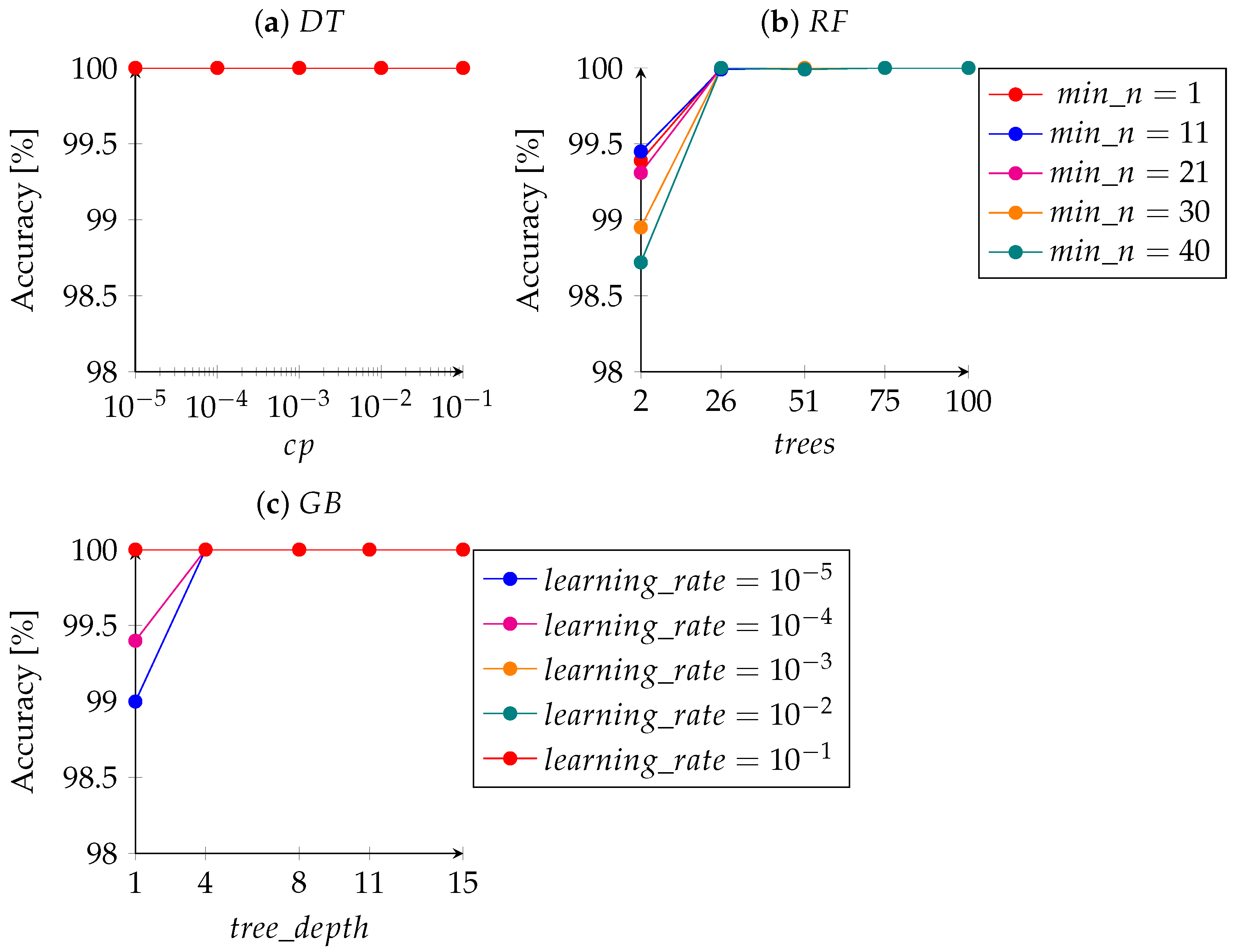
Figure 2a shows the complexity cost ($cp$) and the average accuracy for each model. It can be seen that the method has 100.00% accuracy in all models. Therefore, it can be inferred that a complex tree (with many branches) is not necessary to classify the crop condition with the parameters obtained from GNSS. Thus, the model with $cp$ equal to 10${}^{-1}$ was chosen.

The hyperparameter values, as well as the accuracy of the built models for the RF method are shown in Figure 2b. We can observe that there is less than a 1% difference in the accuracy when varying the number of samples needed to enable a new tree partition ($min\_n$). For the hyperparameter $trees$, there is less than 2% difference in accuracy between using two classifiers ($trees$ = 2) and using more classifiers ($trees$ > 2). Thus, the simplest model with the best accuracy has $trees$ equal to 26 and $min\_n$ equal to 40.

Figure 2c depicts the hyperparameter values as well as the accuracy of the GB models. Less than 1% difference in the predictive capacity of the models can be noted when the hyperparameters $tree\_depth$ and $learning\_rate$ were varied. Based on this, the model with the hyperparameters $learning\_rate$ equal to 10${}^{-5}$, and $tree\_depth$ equal to 4 were chosen.

To choose the best classification technique for external predictor variables of the GNSS sensor, we analysed the execution time and accuracy of the test data, as presented in Figure 3. The technique that has the best performance in terms of processing time is the MLR, with 7.62 $\mathsf{\mu }$s. When the accuracy of the test data was observed, the performance was equal to 100%. In this context, MLR was considered the best technique, as it had the shortest processing time.

3.2. LiDAR

For the MLR technique, there were two models: Total Model (which has all the predictor variables) and Stepwise Model (which has only the variables that present the value of AIC). The characteristics of each of these models can be seen in

Table 10. Comparison between MLR models, using LiDAR data.

Characteristics	Total Model	Stepwise Model
${\beta }_{{\mu }_X}$	✔	✔
${\beta }_{{\sigma }_X}$	✔	✔
${\beta }_{{\gamma }_X}$	✔	✔
${\beta }_{{\mu }_Y}$	✔	✔
${\beta }_{{\sigma }_Y}$	✔	-
${\beta }_{{\gamma }_Y}$	✔	✔
${\beta }_{{\mu }_I}$	✔	✔
${\beta }_{{\sigma }_I}$	✔	-
${\beta }_{{\gamma }_I}$	✔	✔
Accuracy [%]	70.22	70.84
AIC	1546.41	1541.36
LL	−753.21	−754.68
DOF	20	16
LRT	2.944
p-value	0.57

.

The Total Model generated an LL of −753.21 and an AIC of 1546.41. On the other hand, when running the stepwise procedure, an LL of −754.68 and an AIC of 1541.36 were obtained. Therefore, there is a decrease in both parameters, and it can be inferred that the models present contradictory information since the simplest model (Stepwise Model) does not present the highest logarithm of likelihood. When performing the LRT test to determine whether the models differ for predictive purposes, a p value of 0.66 was obtained, which is greater than 0.05; this implies that the null hypothesis cannot be rejected, thus we do not have evidence that the Total Model is better than the Stepwise Model at a significance level of 5%. As we may not accept the alternative hypothesis, the Stepwise Model was chosen because it has fewer predictor variables and, consequently, reduces the computational cost.

Table 11. MLR coefficients using LiDAR data.

	LiDAROcclusion	LiDARInsideCrop
$\alpha$	−1.32	0.73
${\beta }_{{\mu }_X}$	1.65	0.47
${\beta }_{{\sigma }_X}$	1.78	−0.07
${\beta }_{{\gamma }_X}$	−1.08	−0.09
${\beta }_{{\mu }_Y}$	−2.31	−0.44
${\beta }_{{\sigma }_Y}$	-	-
${\beta }_{{\gamma }_Y}$	0.74	0.33
${\beta }_{{\mu }_I}$	5.75	1.00
${\beta }_{{\sigma }_I}$	-	-
${\beta }_{{\gamma }_I}$	−0.53	−0.82

presents the linear ($\alpha$) and angular coefficients ($\beta$), in each of the classes of the response variable other than the reference class LiDAROutsideCrop, for the best model (Stepwise) to predict the response variable.

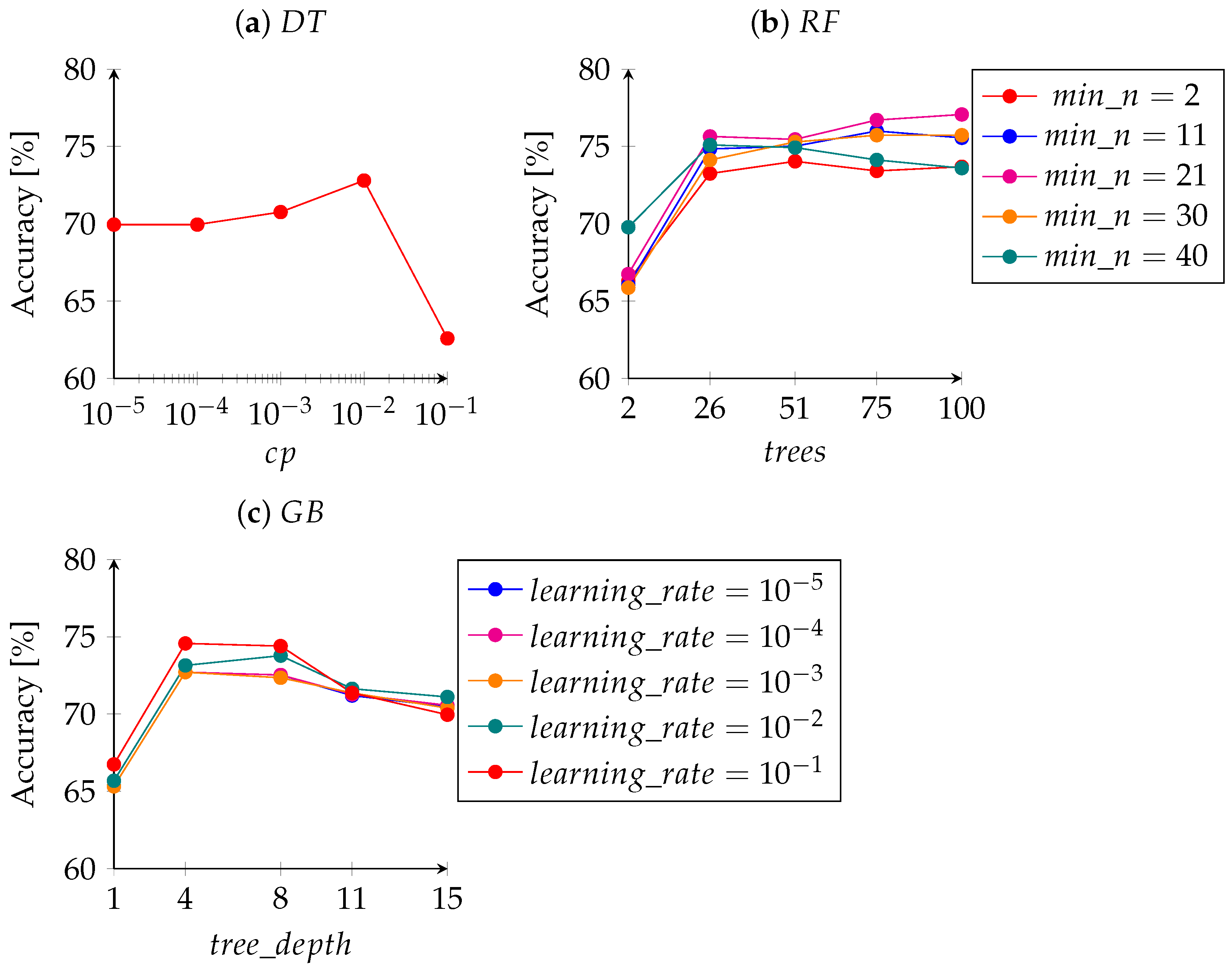
Figure 4a shows the complexity cost ($cp$) and average accuracy for each model. Note that the best accuracy is present when $cp$ is equal to 10${}^{-2}$. After this value, a reduction in the accuracy of the technique was observed, which is an indication of the occurrence of overfitting. Thus, the hyperparameter $cp$ equal to 10${}^{-2}$ was chosen.

The hyperparameter values and the accuracy for the RT models are shown in Figure 4b. For the hyperparameter $min\_n$, a less than 5% difference in the accuracy was observed when varying the number of samples needed to allow a new tree partitioning. However, when analysing the hyperparameter $trees$, it appears that there is an increase in model accuracy by almost 10% when changing this hyperparameter from 2 to 26. Thus, the simplest model with the best accuracy has $trees$ equal to 26 and $min\_n$ equal to 40.

Figure 4c depicts the hyperparameter values and the accuracy for the GB models. For the hyperparameter $tree\_depth$, up to depths 4 and 8, an increase in accuracy was observed followed by a decrease. In the predictive capacity of the models, there was less than 2% difference in the variation of the hyperparameter $learning\_rate$. Thus, the simplest model with the best accuracy has $learning\_rate$ equal to 10${}^{-1}$, and $tree\_depth$ equal to 4.

To choose the best classification technique for external predictor variables of the LiDAR sensor, we analysed the execution time and accuracy of the test data, as presented in Figure 5. The fastest technique in terms of processing time was MLR with 33.33 $\mathsf{\mu }$s. In terms of model accuracy, the best performance was the DT technique with 74.44%. However, to increase the accuracy by 4% with the DT, it was necessary to double the processing time compared to the MLR. In this context, the technique with the best performance in processing (MLR) time was chosen.

3.3. Camera

For the MLR technique, there were two models: Total Model (which has all the predictor variables) and Stepwise Model (which has only the variables that present the value of AIC). The characteristics of each of these models are presented in

Table 12. Comparison between MLR models using camera data.

Characteristics	Total Model	Stepwise Model
${\beta }_{{\mu }_G}$	✔	✔
${\beta }_{{\sigma }_G}$	✔	✔
${\beta }_{{\gamma }_G}$	✔	✔
${\beta }_{{\sigma }_{lap}^2}$	✔	✔
Accuracy [%]	93.76	93.76
AIC	1619.65	1619.65
LL	−789.83	−789.83
DOF	20	20
LRT	0
p-value	1.00

. As can be seen, it is not possible to remove a variable to maintain or increase the predictive capacity of the Total Model; therefore, the Total Model is equal to the Stepwise Model.

Table 13. MLR coefficients using camera data.

	Ideal	HighBrightness	CameraOcclusion	LowBrightness
$\alpha$	2.01	−4.53	1.56	−13.18
${\beta }_{{\mu }_G}$	−3.53	17.31	−2.98	−13.11
${\beta }_{{\sigma }_G}$	−8.72	2.65	−2.09	−2.22
${\beta }_{{\gamma }_G}$	−1.85	−1.25	11.00	10.78
${\beta }_{{\sigma }_{lap}^2}$	17.95	10.01	6.44	16.83

presents the linear ($\alpha$) and angular coefficients ($\beta$) in each of the classes of the response variable, except for the reference class Blur, for the best model (Total) to predict the response variable.

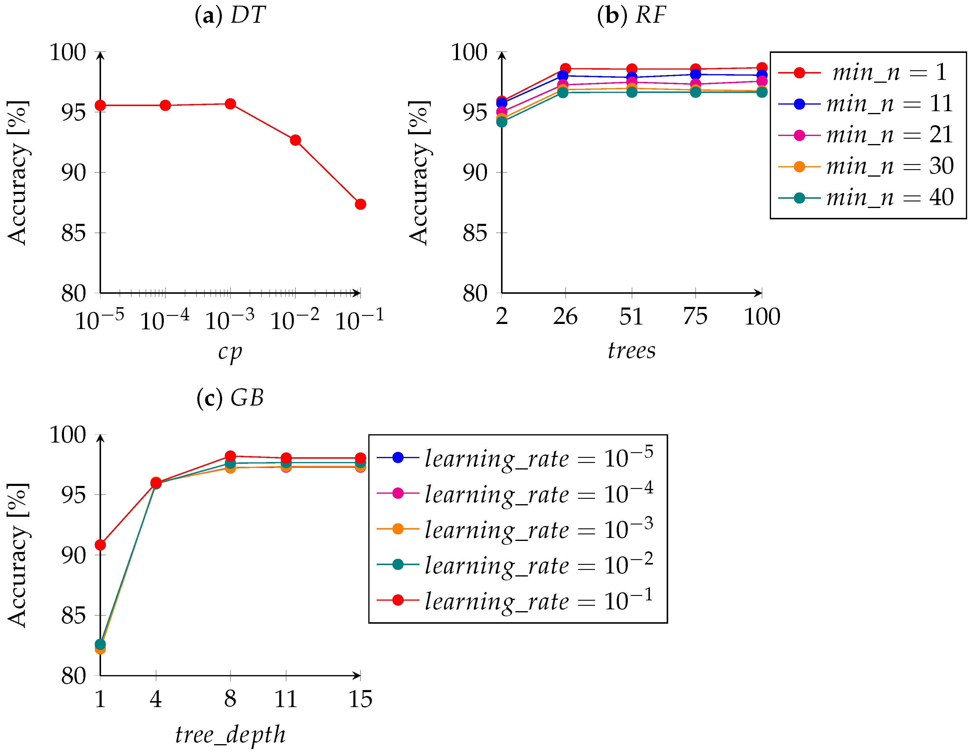
For the DT technique, there were five models chosen. Figure 6a shows the complexity cost ($cp$) and average accuracy for each model. It can be noted that model accuracy increases until a $cp$ value of 10${}^{-3}$, after this value, the accuracy of the model starts to decrease, which is an indication that the model is overfitting to the training data. Thus, the model with a $cp$ equal to 10${}^{-3}$ was chosen.

The hyperparameter values as well as the accuracy of the built models for the RF method are shown in Figure 6b. When analysing the hyperparameter $min\_n$, a 2% difference in accuracy can be seen for simple and complex trees. For the hyperparameter $trees$, there is an increase in the predictive capacity when using 26 classifiers. However, when increasing the number of trees, a constant accuracy was observed, indicating that the model is more complex but without gaining predictive capacity. Thus, the model with $trees$ equal to 26 and $min\_n$ equal to 1 was chosen as the best model.

Figure 6c shows the hyperparameter values and the accuracy of the built models for the GB method. Note that changing the hyperparameter $learning\_rate$ increased the accuracy of the model by about 8%. On the other hand, for the hyperparameter $tree\_depth$, a a higher predictive capacity was observed with a depth equal to 8. After this, the accuracy remained constant. Thus, the best model is the one with $learning\_rate$ equal to 10${}^{-5}$, and $tree\_depth$ equal to 8.

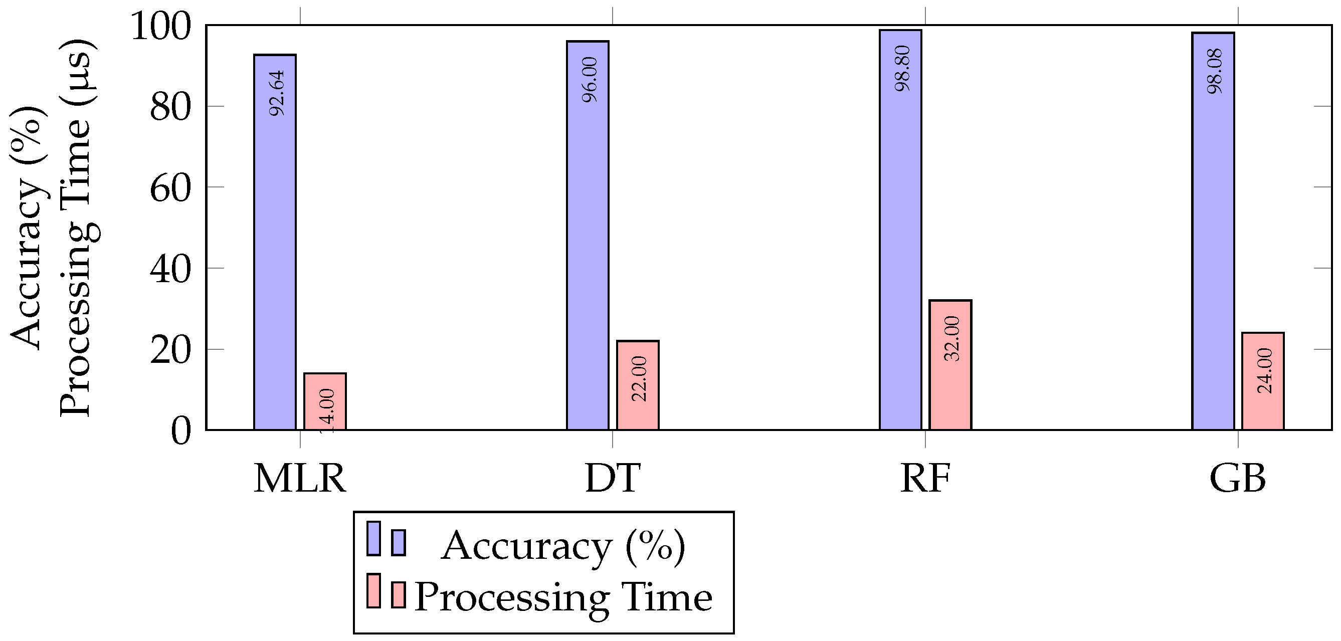
To choose the best classification technique for external predictor variables of camera data, we analysed the execution time and accuracy of the test data, as presented in Figure 7. The fastest technique in terms of processing time was MLR, with 14 $\mathsf{\mu }$s. Regarding the accuracy of the model, the best performance was for the RF technique, with an accuracy equal to 98.80%, and the worst processing time, 32 $\mathsf{\mu }$s. In this context, the GB was judged to be the best technique because it had the second-best accuracy (98.08%) and the third best processing time (24 $\mathsf{\mu }$s).

3.4. Navigation Selections or Navigation Methodologies

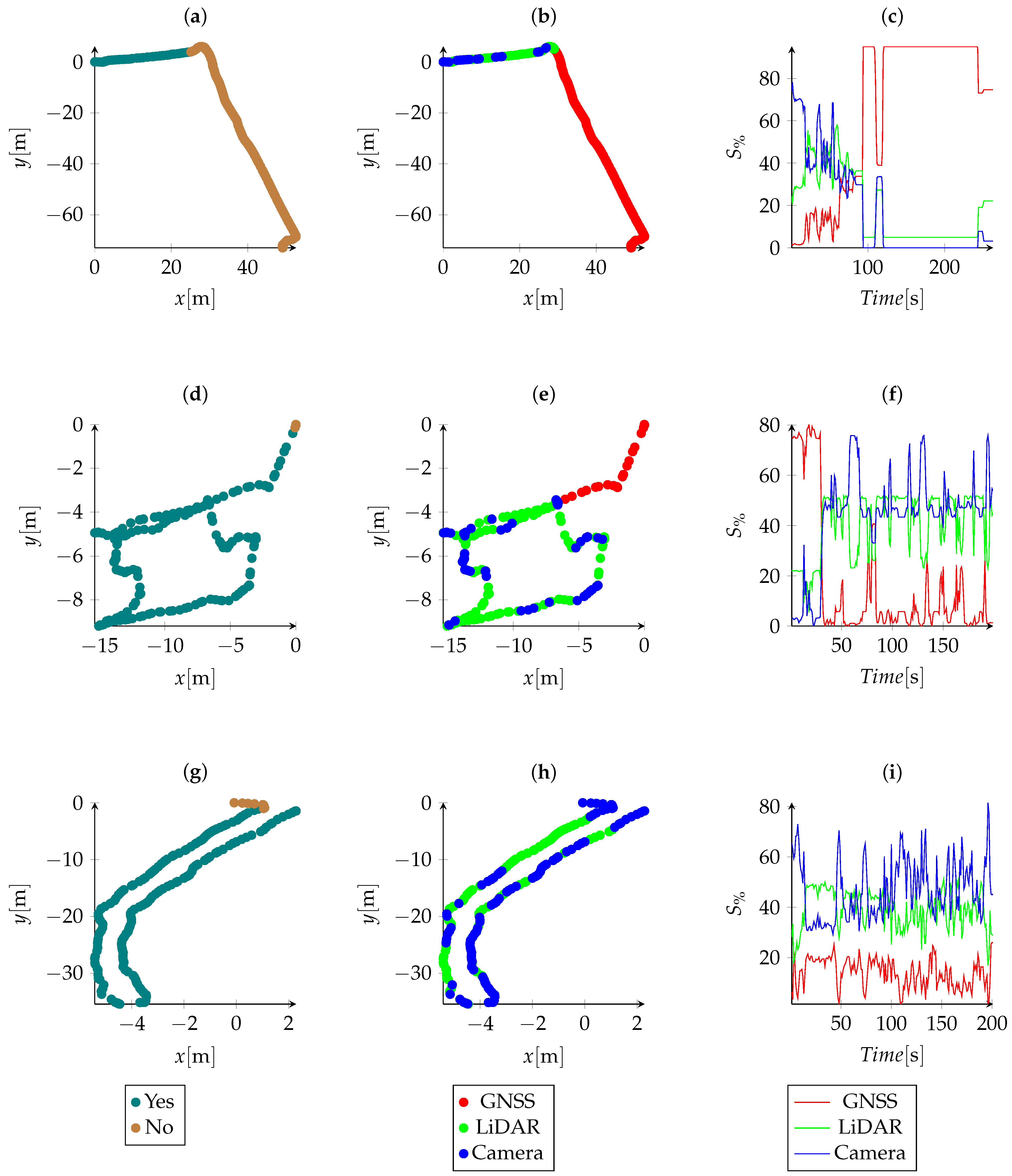
Finally, to validate the methodology for selecting navigation strategies, three runs were performed with the AgBot TS2020.

In Figure 8a, a route was adopted in which the TS2020 went from InsideCrop to OutsideCrop. In Figure 8d, a route was adopted in which the TS2020 went from OutsideCrop to InsideCrop. In Figure 8g, a route was adopted in which the TS2020 went from OutsideCrop to UnderCanopy.

When the platform was navigating within the crop, the robot used LiDAR and the camera to select navigation strategies, as shown in Figure 8b. When analysing the region where there was crops, as shown in

Table 14. Sensors’ selection using feasibility matrix.

Crop?	InsideCrop to OutsideCrop		OutsideCrop to InsideCrop		OutsideCrop to UnderCanopy
	GNSS	LiDAR or Camera	GNSS	LiDAR or Camera	GNSS	LiDAR or Camera
Yes	0	70	24	165	0	192
No	170	23	10	0	0	9

, a navigation strategy using LiDAR or the camera was always selected. However, when analysing the region where there was no crops, a navigation strategy using GNSS was selected 88.08% of the time. After leaving the crops, there was no immediate change in the selected strategy for a period of approximately 20 s (Figure 8b), which is the time it takes for the GNSS sensor to have more weight than the other sensors.

In Figure 8f it is observed, that, similarly to Figure 8c, the navigation strategy using GNSS took approximately 20 s to lose importance in relation to the other navigation strategies. When navigating within the crops, it was observed that, for this condition, there was a level of variation between the navigation strategies that used LiDAR and the camera. The difference in choice between the navigation strategies was, in general, due to sensor occlusions. In addition, it can be seen how much information from the GNSS sensor was omitted due to information from the other sensors. As shown in Table 14, for InsideCrop scenarios, a navigation strategy using LiDAR or the camera was selected in 87.30% of the time. On the other hand, for OutsideCrop scenarios, the selected navigation strategy was GNSS every time.

In Figure 8h, after the period of 20 s, we saw that navigation strategies using GNSS lost importance in relation to the other navigation strategies. The AgBot proximity to the crop, about 1 m, was already enough to indicate that the GNSS sensor should be omitted due to the increase in the horizontal position error. On this route, only navigation strategies that used LiDAR and the camera were selected. In this scenario, it was observed that even within the crops, the strategy using GNSS obtained, on several occasions, an importance of almost 20%. This caused the importance of other strategies to lose magnitude.

4. Conclusions

This paper investigated how to develop a methodology that selects navigation strategies in an AgBot based on the identification of limitations in sensor data. Experimental results showed that the proposed methodology was able to select the optimal navigation strategy for several different scenarios at least 87% of the time.

First, several sensor characteristics were analysed and the best classifier was selected among MLR, DT, RF, and GB to identify how sensor variables can indicate their limitations. Next, a logic of combining the responses of the classifiers was proposed to select the best navigation strategy.

For the GNSS sensor, the classifier with the best performance was MLR, obtaining an accuracy of 100% in all iterations using the repeated k-fold method. It was found that the GNSS signal was affected by trees in a sugarcane field, both from the side and from above, and because of this, all models have perfect accuracy. For GNSS navigation, it was also observed that the algorithm presented better horizontal accuracy in situations of lateral obstruction when compared to superior obstruction. As GNSS data are sensitive to the position of the satellites, it is indicated that future work could investigate the behaviour of horizontal accuracy using data collected throughout the year. The features obtained from the LiDAR point cloud produced a good classifier using MLR, with an accuracy of 70.93%. Furthermore, for variables using the camera sensor, GB was the best model, with an accuracy of 98.08%.

The fusion of data using the viability matrix generated consistent results, giving importance to different navigation strategies depending on the limitations indicated by the classifiers. The normalization of rows and columns allowed removing the bias of the sensor that had the highest number of favourable classes.

Furthermore, the methodology follows the line of a decision-making process based on data, so whenever it is applied to other cultures, new samples must be produced to adapt the classifiers. For this reason, one of the first steps of the methodology is to verify the need to generate a new model.

It was observed that the GNSS signal takes about 20 s to decrease or increase the horizontal accuracy. This can generate a navigation problem; therefore, as future work, the behaviour of the system should be investigated using the Saaty’s scale, as is performed in the analytical hierarchical process to weigh the classes of each classifier with the sensor being analysed.

References

- Tantalaki, N.; Souravlas, S.; Roumeliotis, M. Data-Driven Decision Making in Precision Agriculture: The Rise of Big Data in Agricultural Systems. J. Agric. Food Inf. 2019, 20, 344–380. [Google Scholar] [CrossRef]
- Sparrow, R.; Howard, M. Robots in agriculture: Prospects, impacts, ethics, and policy. Precis. Agric. 2021, 22, 818–833. [Google Scholar] [CrossRef]
- Thayer, T.C.; Vougioukas, S.; Goldberg, K.; Carpin, S. Routing Algorithms for Robot Assisted Precision Irrigation. In Proceedings of the 2018 IEEE International Conference on Robotics and Automation (ICRA), Brisbane, Australia, 21–25 May 2018; pp. 2221–2228. [Google Scholar] [CrossRef]
- Hoppe, A.; Jefferson, E.; Woodruff, J.; McManus, L.; Phaklides, N.; McKenzie, T. Novel Robotic Approach to Irrigation and Agricultural Land Use Efficiency. In Proceedings of the 2022 IEEE Conference on Technologies for Sustainability (SusTech), Sunny Riverside, CA, USA, 21–23 April 2022; pp. 181–186. [Google Scholar] [CrossRef]
- Quan, L.; Jiang, W.; Li, H.; Li, H.; Wang, Q.; Chen, L. Intelligent intra-row robotic weeding system combining deep learning technology with a targeted weeding mode. Biosyst. Eng. 2022, 216, 13–31. [Google Scholar] [CrossRef]
- Alam, M.S.; Alam, M.; Tufail, M.; Khan, M.U.; Güneş, A.; Salah, B.; Nasir, F.E.; Saleem, W.; Khan, M.T. TobSet: A New Tobacco Crop and Weeds Image Dataset and Its Utilization for Vision-Based Spraying by Agricultural Robots. Appl. Sci. 2022, 12, 1308. [Google Scholar] [CrossRef]
- Gao, X.; Li, J.; Fan, L.; Zhou, Q.; Yin, K.; Wang, J.; Song, C.; Huang, L.; Wang, Z. Review of wheeled mobile robots’ navigation problems and application prospects in agriculture. IEEE Access 2018, 6, 49248–49268. [Google Scholar] [CrossRef]
- Bechar, A.; Vigneault, C. Agricultural robots for field operations: Concepts and components. Biosyst. Eng. 2016, 149, 94–111. [Google Scholar] [CrossRef]
- Vougioukas, S.G. Agricultural Robotics. Annu. Rev. Control. Robot. Auton. Syst. 2019, 2, 365–392. [Google Scholar] [CrossRef]
- Siegwart, R.; Nourbakhsh, I.R.; Scaramuzza, D. Introduction to Autonomous Mobile Robots; MIT Press: Cambridge, MA, USA, 2011. [Google Scholar]
- Reitbauer, E.; Schmied, C. Bridging GNSS Outages with IMU and Odometry: A Case Study for Agricultural Vehicles. Sensors 2021, 21, 4467. [Google Scholar] [CrossRef] [PubMed]
- Kaswan, K.S.; Dhatterwal, J.S.; Baliyan, A.; Jain, V. Special Sensors for Autonomous Navigation Systems in Crops Investigation System. In Virtual and Augmented Reality for Automobile Industry: Innovation Vision and Applications; Hassanien, A.E., Gupta, D., Khanna, A., Slowik, A., Eds.; Springer International Publishing: Cham, Switzerland, 2022; pp. 65–86. [Google Scholar] [CrossRef]
- Winterhalter, W.; Fleckenstein, F.; Dornhege, C.; Burgard, W. Localization for precision navigation in agricultural fields—Beyond crop row following. J. Field Robot. 2021, 38, 429–451. [Google Scholar] [CrossRef]
- Fountas, S.; Mylonas, N.; Malounas, I.; Rodias, E.; Hellmann Santos, C.; Pekkeriet, E. Agricultural Robotics for Field Operations. Sensors 2020, 20, 2672. [Google Scholar] [CrossRef]
- Oliveira, L.F.P.; Moreira, A.P.; Silva, M.F. Advances in Agriculture Robotics: A State-of-the-Art Review and Challenges Ahead. Robotics 2021, 10, 52. [Google Scholar] [CrossRef]
- Sigrist, P.; Coppin, P.; Hermy, M. Impact of forest canopy on quality and accuracy of GPS measurements. Int. J. Remote Sens. 1999, 20, 3595–3610. [Google Scholar] [CrossRef]
- Yoshimura, T.; Hasegawa, H. Comparing the precision and accuracy of GPS positioning in forested areas. J. For. Res. 2003, 8, 147–152. [Google Scholar] [CrossRef]
- Chan, C.W.; Schueller, J.K.; Miller, W.M.; Whitney, J.D.; Cornell, J.A. Error Sources Affecting Variable Rate Application of Nitrogen Fertilizer. Precis. Agric. 2004, 5, 601–616. [Google Scholar] [CrossRef]
- Deng, Y.; Shan, Y.; Gong, Z.; Chen, L. Large-Scale Navigation Method for Autonomous Mobile Robot Based on Fusion of GPS and Lidar SLAM. In Proceedings of the 2018 Chinese Automation Congress (CAC), Xi’an, China, 30 November–2 December 2018; pp. 3145–3148. [Google Scholar] [CrossRef]
- Moeller, R.; Deemyad, T.; Sebastian, A. Autonomous Navigation of an Agricultural Robot Using RTK GPS and Pixhawk. In Proceedings of the 2020 Intermountain Engineering, Technology and Computing (IETC), Orem, UT, USA, 2–3 October 2020; pp. 1–6. [Google Scholar] [CrossRef]
- Manish, R.; Lin, Y.C.; Ravi, R.; Hasheminasab, S.M.; Zhou, T.; Habib, A. Development of a Miniaturized Mobile Mapping System for In-Row, Under-Canopy Phenotyping. Remote Sens. 2021, 13, 276. [Google Scholar] [CrossRef]
- Higuti, V.A.H.; Velasquez, A.E.B.; Magalhaes, D.V.; Becker, M.; Chowdhary, G. Under canopy light detection and ranging-based autonomous navigation. J. Field Robot. 2019, 36, 547–567. [Google Scholar] [CrossRef]
- Higuti, V.A.H. 2D LiDAR-Based Perception for under Canopy Autonomous Scouting of Small Ground Robots within Narrow Lanes of Agricultural Fields. Ph.D. Thesis, Universidade de São Paulo, São Paulo, Brazil, 2021. [Google Scholar]
- Weiss, U.; Biber, P. Semantic place classification and mapping for autonomous agricultural robots. In Proceedings of the 2010 IEEE/RSJ International Conference on Intelligent Robots and Systems (IROS) Workshop: Semantic Mapping and Autonomous Knowledge Acquisition, Taipei, Taiwan, 18–22 October 2010. [Google Scholar]
- Ji, T.; Vuppala, S.T.; Chowdhary, G.; Driggs-Campbell, K. Multi-modal anomaly detection for unstructured and uncertain environments. arXiv 2020, arXiv:2012.08637. [Google Scholar] [CrossRef]
- Suh, H.K.; Hofstee, J.W.; van Henten, E.J. Improved vegetation segmentation with ground shadow removal using an HDR camera. Precis. Agric. 2018, 19, 218–237. [Google Scholar] [CrossRef] [Green Version]
- Sunil, G.C.; Zhang, Y.; Koparan, C.; Ahmed, M.R.; Howatt, K.; Sun, X. Weed and crop species classification using computer vision and deep learning technologies in greenhouse conditions. J. Agric. Food Res. 2022, 9, 100325. [Google Scholar] [CrossRef]
- Gasparino, M.V.; Sivakumar, A.N.; Liu, Y.; Velasquez, A.E.B.; Higuti, V.A.H.; Rogers, J.; Tran, H.; Chowdhary, G. WayFAST: Navigation with Predictive Traversability in the Field. IEEE Robot. Autom. Lett. 2022, 7, 10651–10658. [Google Scholar] [CrossRef]
- Preti, M.; Verheggen, F.; Angeli, S. Insect pest monitoring with camera-equipped traps: Strengths and limitations. J. Pest Sci. 2021, 94, 203–217. [Google Scholar] [CrossRef]
- Barbedo, J.G.A. A review on the main challenges in automatic plant disease identification based on visible range images. Biosyst. Eng. 2016, 144, 52–60. [Google Scholar] [CrossRef]
- Mirbod, O.; Choi, D.; Thomas, R.; He, L. Overcurrent-driven LEDs for consistent image colour and brightness in agricultural machine vision applications. Comput. Electron. Agric. 2021, 187, 106266. [Google Scholar] [CrossRef]
- Silwal, A.; Parhar, T.; Yandun, F.; Baweja, H.; Kantor, G. A Robust Illumination-Invariant Camera System for Agricultural Applications. In Proceedings of the 2021 IEEE/RSJ International Conference on Intelligent Robots and Systems (IROS), Prague, Czech Republic, 27 September–1 October 2021; pp. 3292–3298. [Google Scholar] [CrossRef]
- Torres, C.J. Sistema de Controle e Supervisão para Robô Agrícola Móvel Baseado em Fusão de Dados Sensoriais. Ph.D. Thesis, Universidade de São Paulo, São Paulo, Brazil, 2018. [Google Scholar]
- Muñoz-Bañón, M.Á.; del Pino, I.; Candelas, F.A.; Torres, F. Framework for fast experimental testing of autonomous navigation algorithms. Appl. Sci. 2019, 9, 1997. [Google Scholar] [CrossRef] [Green Version]
- Eiffert, S.; Wallace, N.D.; Kong, H.; Pirmarzdashti, N.; Sukkarieh, S. Experimental evaluation of a hierarchical operating framework for ground robots in agriculture. In Proceedings of the International Symposium on Experimental Robotics, La Valletta, Malta, 9–12 November 2020; Springer: Berlin/Heidelberg, Germany; pp. 151–160. [Google Scholar] [CrossRef]
- FAOSTAT. FAOSTAT Statistics Database; FAOSTAT: Rome, Italy, 2022. [Google Scholar]
- Silva, D.L.G.; Batisti, D.L.S.; Ferreira, M.J.G.; Merlini, F.B.; Camargo, R.B.; Barros, B.C.B. Cana-de-açúcar: Aspectos econômicos, sociais, ambientais, subprodutos e sustentabilidade. Res. Soc. Dev. 2021, 10, e44410714163. [Google Scholar] [CrossRef]
- Zhou, M.; Cheng, W.; Huang, H.; Chen, J. A Novel Approach to Automated 3D Spalling Defects Inspection in Railway Tunnel Linings Using Laser Intensity and Depth Information. Sensors 2021, 21, 5725. [Google Scholar] [CrossRef] [PubMed]
- Papoulis, A.; Pillai, S.U. Probability, Random Variables, and Stochastic Processes; Tata McGraw-Hill Education: New York, NY, USA, 2002. [Google Scholar]
Figure 1.
Methodology adopted in the present work.
Figure 2.
Comparison among models using GNSS data: (a) Decision Tree; (b) Random Forest; and (c) Gradient Boosting.
Figure 3.
Comparison among techniques using GNSS data.
Figure 4.
Comparison among models using LiDAR data: (a) Decision Tree; (b) Random Forest; and (c) Gradient Boosting.
Figure 5.
Comparison among techniques using LiDAR data.
Figure 6.
Comparison among models using camera data: (a) Decision Tree; (b) Random Forest; and (c) Gradient Boosting.
Figure 7.
Comparison among techniques using camera data.
Figure 8.
Trajectory: (a) InsideCrop to OutsideCrop: Presence of crop; (b) InsideCrop to OutsideCrop: Selection of sensors for navigation; (c) InsideCrop to OutsideCrop: Probability indicated by the methodology of selecting each navigation strategy; (d) OutsideCrop to InsideCrop: Presence of crop; (e) OutsideCrop to InsideCrop: Selection of sensors for navigation; (f) OutsideCrop to InsideCrop: Probability indicated by the methodology of selecting each navigation strategy; (g) OutsideCrop to UnderCanopy: Presence of crop, (h) OutsideCrop to UnderCanopy: Selection of sensors for navigation and (i) OutsideCrop to UnderCanopy: Probability indicated by the methodology of selecting each navigation strategy.