BMAE-Net: A Data-Driven Weather Prediction Network for Smart Agriculture

Abstract

Weather is an essential component of natural resources that affects agricultural production and plays a decisive role in deciding the type of agricultural production, planting structure, crop quality, etc. In field agriculture, medium- and long-term predictions of temperature and humidity are vital for guiding agricultural activities and improving crop yield and quality. However, existing intelligent models still have difficulties dealing with big weather data in predicting applications, such as striking a balance between prediction accuracy and learning efficiency. Therefore, a multi-head attention encoder-decoder neural network optimized via Bayesian inference strategy (BMAE-Net) is proposed herein to predict weather time series changes accurately. Firstly, we incorporate Bayesian inference into the gated recurrent unit to construct a Bayesian-gated recurrent units (Bayesian-GRU) module. Then, a multi-head attention mechanism is introduced to design the network structure of each Bayesian layer, improving the prediction applicability to time-length changes. Subsequently, an encoder-decoder framework with Bayesian hyperparameter optimization is designed to infer intrinsic relationships among big time-series data for high prediction accuracy. For example, the R-evaluation metrics for temperature prediction in the three locations are 0.9, 0.804, and 0.892, respectively, while the RMSE is reduced to 2.899, 3.011, and 1.476, as seen in Case 1 of the temperature data. Extensive experiments subsequently demonstrated that the proposed BMAE-Net has overperformed on three location weather datasets, which provides an effective solution for prediction applications in the smart agriculture system.

1. Introduction

Agriculture is essential for people’s livelihoods and is vital for the world’s food supply. The yield of crops is directly dependent on natural resources and is closely related to changing weather patterns. Weather resources affect the agricultural production environment, crop-planting layouts, crop yield, and even food trade security. Especially in field agriculture, the land is exposed to the outdoor environment, and weather changes directly affect the crops’ growth.

Accurate agricultural environment prediction can guide farming operations and provide good crop-growing conditions. In an environment of global weather changes, the frequent occurrence of extreme weather causes crop damage and yield reduction. Weather prediction can also guide producers in coping with the greenhouse effect, natural disaster prevention, etc. [1]. While the performance of current weather time series prediction models cannot be accommodated using different time durations and locations, the ability to generalize data to other regional datasets needs to be improved. Meanwhile, as the model’s complexity increases, many hyperparameters need to be adjusted, significantly reducing its operational efficiency; therefore, it needs to be more lightweight because it is otherwise challenging to deploy in practical applications [2,3].

Traditionally, weather prediction is performed by establishing partial differential equations (PDEs) to simulate the physical processes of atmospheric changes and applying numerical means to solve differential equations and, thus, achieve predictions. In recent decades, the prediction performance of this method has gradually improved; now, not only temperature changes but also precipitation and hurricane tracks can be predicted [4]. As the demand for prediction accuracy has become higher, scientists have further improved accuracy by fine-tuning the physical parameters and improving the power core, but this elicits high computational costs [2].

The rapid development of IoT sensor technology and cloud storage technology has brought convenience to agricultural production. By collecting real-time information, agricultural IoT provides timely control of the agricultural production process and establishes a high-quality, high-yielding, and efficient agricultural production management model to ensure the quantity and quality of agricultural products [5]. Sensor devices can collect various environmental factors in farmland in real time, sort them in chronological order, and form specific time series data—for example, meteorological data, soil data, and environmental data—in modern intelligent agricultural greenhouses [6,7,8,9]. Time series forecasting uses data mining and data analysis methods to extract a correlation between data, predict changes in the future, and then provide production planning and designation decisions. For example, meteorological researchers predict temperature, humidity, and wind direction based on historical meteorological data, cloud images, and environmental monitoring equipment to provide information for production and people’s daily life [10]. In the modern smart agricultural greenhouse [11,12], the temperature, air humidity, soil humidity, and light intensity are monitored, and the environmental data are modeled and predicted. The greenhouse environment is regulated to provide a better crop-growth environment and improve crop quality and yield. Therefore, time series forecasting has important practical significance and research value, and more accurate forecasting is an essential research direction of time series forecasting.

With the advent of big data, time series data present nonlinear characteristics and randomness, which puts forward new requirements for time series forecasting [13]. An important and meaningful area of research is how to model time series and reliably predict the development trend accurately.

Traditional forecasting methods analyze time series data based on probability and statistics. However, they are limited by prior knowledge, and the model prediction accuracy and generalization are not good enough. When the data are nonlinear and contain noise, it is difficult for traditional time series forecasting methods to achieve good nonlinear fitting for such complex data. Meanwhile, data-driven machine learning is developing rapidly. Machine learning digs out hidden data rules from historical data to realize the prediction of time series data. However, machine learning is often insufficient when the data are limited and incomplete. Deep neural networks have recently been widely used, especially for multi-step prediction. Standard deep neural network (DNN) models, such as convolution neural networks (CNN), long short-term memory (LSTM), gated recurrent units (GRU), encoder-decoder, and transformer models, have been commonly used in computer vision [14], image classification [15], time series prediction [16], natural language processing [17], and other fields. Compared to methods for building PDEs, deep learning demonstrates powerful modeling capabilities with large datasets that can be deployed on modern computer systems. However, neural networks are prone to learning pseudo-relationships in the data because of the lack of consideration of physical constraints.

From the above survey, the following can be seen:

(1)

It is well known that time series data have the characteristics of solid volatility and randomness, and their complex features require the model to have strong feature extraction capabilities. At the same time, there are errors in the process of reading data by sensors because the noise in the environment may change the readings, which will significantly affect the prediction performance, requiring a deep neural network for in-depth mining.

(2)

Most traditional models are used for single-step prediction, and the encoded vector information will be lost when the input sequence is too long. Therefore, the existing models cannot achieve medium- and long-term forecasting and are limited in practical application and early warning.

In response to the above two problems, a multi-head attention encoder-decoder neural network, optimized via Bayesian inference strategy (BMAE-Net), has been designed to predict weather time series changes accurately. The overall contribution of this framework is threefold:

(1)

The existing prediction models cannot accommodate different prediction steps, and there are differences in the prediction performance of the models at extra prediction steps. Therefore, we integrated Bayesian variational inference into the GRU and multi-headed attention layers to effectively improve the causal inference capability to model weather time series. The model can adapt to different prediction steps and still maintain excellent performance, i.e., it maintains an advantage in the time dimension.

(2)

The existing models must be more robust across different datasets, especially in weather prediction. The temperature varies significantly from location to location; the same model has variable prediction accuracy on time series data from different areas. Therefore, this paper introduces a codec framework that uses Bayesian-GRU as the encoder and decoder and incorporates a Bayesian multi-head attention (BMA) layer in between to construct the BMAE-Net. This framework achieves better prediction performance on different regional datasets and exceeds the baseline model in terms of spatial dimensionality and generalizability.

(3)

It is time-consuming and laborious to tune the parameters by hand and the model needs self-adaptability. Relying on a Bayesian optimization strategy, the model can automatically search for the globally optimal hyperparameter results and adaptively adjust them. The model considers the learning efficiency, stability, and the total number of parameters, which renders it more suitable for IoT-based practical sensor deployment applications and offers broader application prospects [18].

Subsequent chapters of this paper are organized as follows: Section 2 summarizes related work on time series prediction and Bayesian theory. Section 3 expounds on the general architecture of the model and describes the process details. Then, Section 4 presents the experimental results and analysis. Finally, the conclusions of this study are summarized, and future research is discussed.

2. Related Works

2.1. Data-Driven Time Series Forecasting Models

Traditional time series forecasting methods include statistical methods, machine learning, and deep neural networks. Statistical methods mainly use mathematical analysis methods to describe time series data and establish mathematical models through statistical probability methods to collect historical event trends. Traditional time series forecasting methods include the autoregressive model, autoregressive moving average (ARMA) model, differential autoregressive moving average (ARIMA) model, etc. Zeng et al. [19] combined ARMA with a backpropagation (BP) neural network to design a combined optimization model for wind power prediction. Wang et al. [20] used ARIMA to predict short-term cloud coverage, while Chen [21] used a generalized autoregressive conditional heteroskedasticity model to predict power generation. However, these statistical models require the data to be a stationary time series. The model parameters must rely on human experience, so they are unsuitable for fitting nonlinear series.

Compared with statistical methods, machine learning continuously adjusts parameters through an internal iteration of the model, which is more suitable for nonlinear fitting problems, such as the backpropagation (BP) model. For example, Xiao [22] designed a rough set BP model for the premise prediction of short-term load to overcome the effect of noise on prediction accuracy. In addition, multilayer perceptron (MLP) [23], support vector machine (SVM) [24], and hidden Markov models [25] have all been used in time series forecasting.

With the development of computer technology, DNNs that can process complex information have been established. Many capabilities, such as fault detection, speech recognition, natural language processing (NLP), and disease diagnosis, have shown excellent performance [26]. Recurrent neural networks (RNN) structurally consider the timing of the data, establish connections in the hidden layer, and have a better nonlinear fitting ability. Nevertheless, traditional RNNs suffer from the problem of vanishing gradients, so it is challenging to capture long-term dependencies. Long short-term memory networks (LSTMs) and gated recurrent units (GRUs) have overcome this limitation in recent years [27]. An LSTM network has multiple gated structures to improve the gradient disappearance and long-term dependence problems of traditional RNNs. Li [28] fused multi-feature attention, temporal attention, and LSTM to propose an attention-aware LSTM model for soil temperature and humidity prediction. GRUs reduce the number of gated units based on LSTM, have a more straightforward network structure and fewer training parameters than LSTM, and improve the operation speed while achieving the same effect. Jin [29] integrated empirical model decomposition and gated recurrent units to design a combined model for premise prediction of temperature, humidity, and wind speed for decision-making in precision agricultural production. Although machine learning has achieved good results in nonlinear fitting, its noisy data prediction performance still needs improvement.

2.2. Attention-Based Encoder-Decoder Prediction Methods

The encoder-decoder framework was first applied to text processing and consisted of two parts, the encoder, and the decoder, also known as end-to-end or sequence-to-sequence systems. The encoder is responsible for mapping the input sequence data into a fixed-length encoding vector, while the decoder is responsible for decoding the encoding vector into an output sequence [30] that consists of multilayer CNN, RNN, LSTM, and GRU networks. Because of its unique structure and powerful feature extraction capabilities, the encoder-decoder model is widely used in machine translation, time series prediction, and other fields [31,32,33]. However, it also has a problem with information loss, and the model performance will gradually decrease with any increase in the input time series length.

Therefore, the researchers incorporated the attention mechanism into the neural network. The essence of the attention mechanism is to assign weights to sequences, selecting and assigning higher weights to important feature information and filtering out irrelevant feature information. The attention mechanism clarifies the relationship between input and output and enhances the interpretability of the model. It also reduces computational effort because the more information there is to be learned, the more complex the model becomes and the higher the computational power needed for the computer. Meanwhile, the attention mechanism alleviates the vanishing disappearance and gradient explosion. Recently, the attention mechanism has been widely used for time series prediction. Du [34] proposed a temporal attention encoder-decoder model for multivariate time series forecasting. Jin [35] combined wavelet decomposition and a bidirectional LSTM network and integrated the attention mechanism to predict the temperature and humidity of the smart greenhouse. Nandi [36] established a model based on the self-attention mechanism and an encoder-decoder framework to approach long-term air temperature forecasting tasks.

Transformer [37] is a model proposed by Vaswani et al. that is entirely based on the attention mechanism to capture global dependencies. It replaces the standard RNN network structure with a self-attention structure that allows parallel computation and was first applied to NLP. More recently, the transformer model has demonstrated powerful capabilities in temporal sequence prediction, especially in long sequence prediction. In recent years, the transformer model has demonstrated significant advantages in time series prediction. However, as the input sequence length increases, the computational complexity of the classical Transformer is too high. To reduce the computational cost, scholars have proposed a series of variants based on attention mechanisms, such as sparse attention [38], ProbSparse attention [39], and LogSparse attention [40].

2.3. Bayesian Optimization Theory for Time Series Prediction

The Bayesian theorem is intended to deal with uncertainty. Unlike traditional machine learning, the Bayesian theorem derives the posterior distribution, based on the prior distribution and the likelihood function. The Bayesian theorem can be viewed as an information processing system, where the input is the prior distribution and likelihood function, and the output is the posterior distribution of the model. This information theory-based interpretation allows the Bayesian theorem to be more widely applied to time series prediction methods, such as Bayesian neural networks and Bayesian optimizers.

The Bayesian neural network uses Bayesian theory and the variational inference method to introduce an a priori probability into the weight and bias of the neural network. It continuously adjusts the prior probability through backpropagation, thereby extracting the distribution features implicit in the data. It is an inference neural network with uncertainty [41,42]. In ordinary neural networks, fully connected networks are mainly used for data fitting, and the model’s internal parameters are determined values. Although this is convenient for model training, it is prone to overfitting [43]. Unlike a traditional neural network, a Bayesian neural network has a random number that obeys the posterior probability distribution. Thus, using the Bayesian inference method by introducing weights related to conditional probability distributions, Bayesian neural networks can solve the common problem of overfitting seen in classical neural networks [44]. Steinbrener [45] used a variational Bayesian approach to construct a Bayesian linear layer, using it to model the current information along the Pacific coastline to predict the maximum tsunami height. Jin [46] combined Bayesian variational inference with an autoencoder. The model used planar flow to transform the internal features of the variational autoencoder, to propose a temperature predictor that overcomes noise and improves the dynamic adaptability of the model. Park [47] proposed a Bayesian spatiotemporal model to deal with the missing data problem in agrometeorological data. The Bayesian theorem is also used to perform parametric optimization. In recent years, Bayesian optimization has become more and more widely used in solving black-box function problems and has become a mainstream method of hyperparametric optimization [48,49,50]. Dairy et al. [51] reviewed the literature on using Bayesian networks in agricultural research. They showed that Bayesian networks can reason regarding incomplete information and incorporate prior knowledge, so they are well-suited for agricultural research.

Based on the attention mechanism and encoder-decoder framework, we incorporated the Bayesian theorem to construct a BMAE-Net for predicting the weather.

3. Materials and Methods

For this work, we designed a multi-head attention encoder-decoder neural network, optimized via Bayesian inference strategy (BMAE-Net) to accurately predict weather time series changes. The proposed model innovated on the backbone network with an encoder-decoder framework. Then, a multi-head attention mechanism has been adopted to design a novel network structure among neuron layers, improving the network’s compatibility performance for different duration predictions. Subsequently, Bayesian inference theory was introduced into several essential processes of the proposed model, including neural unit designing, network layer connection, and hyperparameter optimization, to improve the learning efficiency and forecasting accuracy comprehensively. A depiction of the model can be seen in Figure 1.

3.1. Bayesian-GRU Module

In a traditional recurrent neural network, the GRU has both the feedback mechanism and the chain structure of hidden units of a traditional RNN and the gate control mechanism of LSTM. At the same time, the number of parameters is fewer, and the feature extraction capacity is more potent. The traditional GRU forward propagation process is as follows [52]:

$$z_t=\sigma (W_z[h_{t-1},x_t]+b_z)$$

(1)

$$r_t=\sigma (W_r[h_{t-1},x_t]+b_r)$$

(2)

$${\tilde{h}}_t=\tanh (W_h[r_t\odot h_{t-1},x_t]+b_h)$$

(3)

$$h_t=(1-z_t)\odot {\tilde{h}}_t+z_t\odot h_{t-1}$$

(4)

where $x_t$ is the input data and $z_t$ and $r_t$ are the output of the update gate and reset gate, respectively. $z_t$ is used to control the amount of data that the previous memory information can continue to retain until the current moment. $r_t$ is used to control how much of the past information is to be forgotten. $h_{t-1}$ indicates the state information of the previous moment, ${\tilde{h}}_t$ is the current candidate hidden state information, and $h_t$ is the current hidden state information; $W_r$, $W_z$, and $W_h$ are the weights of the reset gate, the update gate and hidden state; $b_r$, $b_z$, and $b_h$ are the biases.

Based on its uncertainty estimate, the problem of model overfitting is improved. The Bayesian gated recurrent unit (Bayesian-GRU) is used to sample the network weights through probability density distribution and then optimize the distribution parameters, instead of setting a certain weight in the traditional neural network. In the Bayesian-GRU, $W_r$ and $b_r$ no longer have a specific value, but instead have a sampling point that obeys a Gaussian distribution, with mean ${\mu }_z$ and standard deviation ${\sigma }_z$. The Bayesian-GRU network structure is shown in Figure 2.

We assume that $W_{(n)}^{}$ is the n-th sampling weight and $b_{(n)}^{}$ is the bias, both conforming to the Gaussian distribution. The Gaussian distribution meets the requirement that the mean is $\mu$ and standard deviation is $\sigma$ for the translation and scaling transformation.

$$W_{(n)}^{}=\mathcal{N}\left(0,1\right)\times \log \left(1+\sigma \right)+\mu$$

(5)

$$b_{(n)}^{}=\mathcal{N}\left(0,1\right)\times \log \left(1+\sigma \right)+\mu$$

(6)

The definition of the loss function is as follows:

$$Loss=\log \left(q(\omega |\theta )\right)-\log \left(p(\omega )\right)$$

(7)

where $p(\omega )$ is a priori distribution and $q(\omega |\theta )$ is posterior distribution; this allows the Bayesian-GRU to learn the distribution features. Since the target given during training is a series of fixed values, the loss function consists of a combination of deterministic and uncertainty errors. The loss function of the Bayesian-GRU is as follows:

$$Loss=\alpha \times mse(\widehat{y},y)+\frac{1}{\alpha }\times \left[\log \left(q(\omega |\theta )\right)-\log \left(p(\omega )\right)\right]$$

(8)

where $\widehat{y}$ is the predicted value of the output under the current weight sampling, and $\alpha$ is the weight coefficient, which is equal to the product of the number of training samples and the batch size.

3.2. Bayesian Multi-Head-Attention Module

As the input sequence length increases, the feature information extracted earlier will be overwritten, resulting in the loss of feature information and a decrease in the model’s predictive power. This work improves the existing encoder-decoder framework and proposes a Bayesian multi-head-attention module to solve the information loss problem. This module addresses the prediction of different prediction intervals and enhances the feature extraction ability of the model.

Multi-head attention is a variant of the additive attention-based mechanism. The attention mechanism can be described as a mapping of a query to a series of key-value pairs, with scaled dot product attention at its core, where query, key and value are vectors, and the output is a weighted sum of values, indicating the relevance of the query and the current key pair. We construct the structure of the Bayesian multi-head attention mechanism by transforming the linear layer of multi-head attention into a Bayesian linear layer, as shown in Figure 3.

The Bayesian attention layer consists of a multilayer multi-head attention mechanism. We defined $d=m/h$, $q=k=v=H$, where $h$ is the number of heads. First, the encoder output $H$ is first linear transformed, and then the input of the $i$-th head is $Q_i,K_i,V_i\in {ℝ}^{t\times d}$:

$$\begin{array}{l}{Q}_i={\omega }_{iq}q\\ {\omega }_{iq}^{}=\mathcal{N}\left(0,1\right)\times \log \left(1+{\rho }_q{}^{}\right)+{\mu }_q{}^{}\end{array}$$

(9)

$$\begin{array}{l}{K}_i={\omega }_{ik}k\\ {\omega }_{ik}^{}=\mathcal{N}\left(0,1\right)\times \log \left(1+{\rho }_k{}^{}\right)+{\mu }_k{}^{}\end{array}$$

(10)

$$\begin{array}{l}{V}_i={\omega }_{iv}v\\ {\omega }_{iv}^{}=\mathcal{N}\left(0,1\right)\times \log \left(1+{\rho }_v{}^{}\right)+{\mu }_v{}^{}\end{array}$$

(11)

where ${\mu }_i,{\rho }_i,{\mu }_k,{\rho }_k,{\mu }_v,{\rho }_v$ is the parameter to be learned. The attention weight calculation process is as follows:

$$AttentionWeight=softmax\left(\frac{Q{K}_{}^T}{\sqrt{d}}\right).$$

(12)

The output of the $i$-th head $hea{d}_i\in {ℝ}^{t\times d}$ is as follows:

$$hea{d}_i=Attention(Q,K,V)=softmax\left(\frac{Q_i{K}_i^T}{\sqrt{d}}\right)V_i$$

(13)

where $hea{d}_i$ is the weighted Bayesian encoder output. The output of the $h$ header is concatenated together and is then subjected to Bayesian-linear variation, to obtain the encoding vector, $C\in {ℝ}^{t\times m}$:

$$C={\omega }_c·concat[hea{d}_0;hea{d}_1;\dots ;hea{d}_q]$$

(14)

$${\omega }_c^{}=\mathcal{N}\left(0,1\right)\times \log \left(1+{\rho }_c{}^{}\right)+{\mu }_c{}^{}$$

(15)

where ${\mu }_c,{\rho }_c$ is the parameter to be learned. Bayesian multi-head-attention uses multiple queries to select features in the input information through parallel computing. The essence of Bayesian multi-head attention is to introduce several independent attention mechanisms in parallel, using different weight matrices to linearly transform the query to obtain multiple queries, which can extract the important features in the sequence and prevent overfitting.

The heads of each attention focus on different parts of the input information. The distributed multi-head attention mechanism saves computing resources, reduces computing costs, and improves the computing efficiency of the model.

3.3. Bayesian Encoder-Decoder Framework

Based on the encoder-decoder model, Bayesian-GRU and Bayesian multi-head-attention are integrated to form a sequence-to-sequence (seq-to-seq) Bayesian encoder and decoder framework.

• Data preprocessing. First, a sliding window is applied to the data, $X={[x_1,x_2,\cdots ,x_n]}^T$ is assumed to be time series data, with a feature length of $n$. The input length is $t$, the output length is $\tau$, and the step size is $s$.
• Encoder layer. The Bayesian-GRU is selected as the basic unit of the encoder. After the data are pre-processed, it is transmitted to the Bayesian-GRU for feature encoding. In the BMAE-Net, the Bayesian encoder layer outputs the hidden states at each time step to obtain $H={\left[h_1,h_2,\cdots ,h_t\right]}^T\in {ℝ}^{t\times m}$.
• Bayesian multi-head attention layer. The output obtained from the Bayesian encoder is input to the Bayesian multi-head attention layer, and the attention score is calculated and weighted by Bayesian multi-head attention to obtain Equation (12). Finally, the encoding vector $C={\omega }_c\times concat[hea{d}_0;hea{d}_1;\dots ;hea{d}_q]$ is obtained by splicing and linear transformation.
• Decoder layer. The Bayesian decoder is the same as a Bayesian encoder, which also consists of multiple layers of Bayesian-GRU. The encoding vector is input to the Bayesian decoder, and after passing through the layers, the hidden state of the last time step in the Bayesian decoder is output. A nonlinear transformation is performed to obtain the prediction sequence:

$$\tilde{Y}={\left[{\tilde{y}}_1,{\tilde{y}}_2,\dots {\tilde{y}}_{\tau }\right]}^T=\mathrm{Relu}({\omega }_y{h}^{·}+b_y)$$

(16)

$${\omega }_y^{}=\mathcal{N}\left(0,1\right)\times \log \left(1+{\rho }_y{}^{}\right)+{\mu }_y{}^{}$$

(17)

where ${\mu }_y,{\rho }_y$ is the parameter to be learned, and $\tau$ is the prediction length of the target sequence. $Relu$ is the activation function, with the following expression:

$$Relu(x)=\{\begin{array}{l}x,x>0\\ 0,x\le 0\end{array}.$$

(18)

During model training, the model optimizes the hyperparameters, based on the prediction results and expectations. When an optimal set of hyperparameters is obtained, the optimization process is stopped, and the parameters are applied to the prediction.

3.4. Bayesian-Based Hyperparameter Optimization

Many parameters in the encoder-decoder multi-head attention model directly impact the model’s performance. As the complexity of the model increases, hyperparameter selection becomes a challenging problem, while the correct choice of hyperparameters can ensure the model’s good performance. This paper introduces a Bayesian optimization algorithm (BOA) for hyperparameter optimization. The BOA is an efficient global optimization algorithm, where an objective optimization function is used during the optimization process to optimize the results continuously. The objective optimization function can be expressed as:

$$f(\omega )=\sqrt{\frac{{\displaystyle {\sum }_{i=1}^m{\left({\widehat{y}}_i(\omega )-y_i\right)}^2}}{m}}$$

(19)

where $y_i$ represents the true value, ${\widehat{y}}_i(\omega )$ represents the predicted value, and $m$ is the length of the input time series. The objective function is minimized as:

$${\omega }^{*}=\underset{\omega \in W}{\arg \min }f(\omega )$$

(20)

where $W$ is the set of all parameters, ${\omega }^{*}$ denotes the best parameter obtained, and $\omega$ is a set of hyperparameter combinations.

In the parameter tuning process, a Gaussian function is chosen as the distribution assumption for the prior function. Then, the next point in the posterior process is chosen for evaluation, using the acquisition function. The Gaussian process is an extension of the multidimensional Gaussian distribution and can be defined using the mean and covariance:

$$f(\omega )\sim GP(\mu (\omega ),K(\omega ,{\omega }^{\prime }))$$

(21)

where $\mu (\omega )$ is the mean value of $f(\omega )$ and $K(\omega ,{\omega }^{\prime })$ is the covariance matrix of $f(\omega )$. Initially, it can be expressed as follows:

$$K=\left(\begin{array}{ccc}k({\omega }_1,{\omega }_1)& \dots & k({\omega }_1,{\omega }_i)\\ ⋮& \ddots & ⋮\\ k({\omega }_i,{\omega }_1)& \cdots & k({\omega }_i,{\omega }_i)\end{array}\right).$$

(22)

During the search for optimal parameters, the above covariance matrix changes continuously during the iterations. When new samples are added to the set, the covariance matrix is updated to:

$$K^{\prime }=\left(\begin{array}{cc}K& k^T\\ k& k({\omega }_{i+1},{\omega }_{i+1})\end{array}\right)$$

(23)

$$k=[k({\omega }_{i+1},{\omega }_1),k({\omega }_{i+1},{\omega }_2),\cdots ,k({\omega }_{i+1},{\omega }_i)].$$

(24)

The posterior probabilities can be obtained from the updated covariance matrix:

$$P(f_{i+1}|D_{i+1},{\omega }_{i+1})\sim N({\mu }_{i+1}(\omega ),{\sigma }_{i+1}^2(\omega ))$$

(25)

where $D$ is the observed data, ${\mu }_{i+1}(\omega )$ is the mean value of $f(\omega )$ at step $i+1$, and ${\sigma }_{i+1}^2(\omega )$ is the variance of $f(\omega )$ at step $i+1$.

By evaluating the mean and covariance matrices, the values of the sampled functions from the joint posterior distribution are found to be faster for the final parameters and reduce the wasting of resources. We choose the upper confidence bounds (UCB), as the sampling function:

$$UCB(\omega )=\mu (\omega )+\lambda \sigma (\omega )$$

(26)

$${\omega }_{i+1}=\arg \max UCB=\arg \max \mu (\omega )+{\lambda }_{i+1}{\sigma }_i(\omega )$$

(27)

where $\lambda$ is a constant, ${\omega }_{i+1}$ is the hyperparameter chosen at step $i+1$, and $\mu (\omega )$ and $\sigma (\omega )$ are the mean and covariance of the joint posterior distribution of the objective function obtained in the Gaussian process, respectively.

The algorithm-running process of BMAE-Net, based on Bayesian optimization, is shown in Algorithm 1.

Algorithm 1 Training of the BMAE-Net Model

Input: the weather data, hyperparameter space $W$, epochs

Output: the optimal hyperparameter, the prediction of temperature

1: for i = 1: n do

2:    Select a set of parameters $\omega$ from the hyperparameter space $W$

3:    Train the model with $\omega$

4:    Evaluate model performance with Equation (19)

5:    Update the covariance matrix and calculate the posterior probability

6:    parameters ${\omega }^{*}$ update by $UCB$ function

7: Obtain the best model parameters ${\omega }^{*}$ and predict

4. Experiments

4.1. Datasets and Evaluation Metrics

With economic development and people’s pursuit of a better life, accurate prediction of meteorological data is of practical importance to support agriculture. Temperature variation is closely related to agricultural production and is a major factor affecting the growth and development of crops. Temperature prediction helps in agricultural planning, disaster weather prevention, and the planning of agricultural output, thus improving crop yield and quality and increasing economic growth.

The temperature substantially affects the crop’s distribution and quality, so this experiment uses temperature data collected from meteorological stations in agricultural areas at three locations in China as the study object. The source code is available at https://github.com/btbuIntelliSense/Temperature-and-humidity-dataset (accessed on 29 November 2022). The three cities are located in the northeast, north, and south of China, Shenyang, Beijing, and Guangzhou, and the latest data showed that these three locations have 10.3 million, 1.77 million, and 0.44 million mu (a Chinese unit of area, where 1 mu = 666.7 m²) of grain sown in 2022. The different locations show different temperature variations, meaning that the distribution of crops varies from location to location, with wheat being the main grain crop in Shenyang, maize being grown more in Beijing, and indica rice being the main crop in Guangzhou.

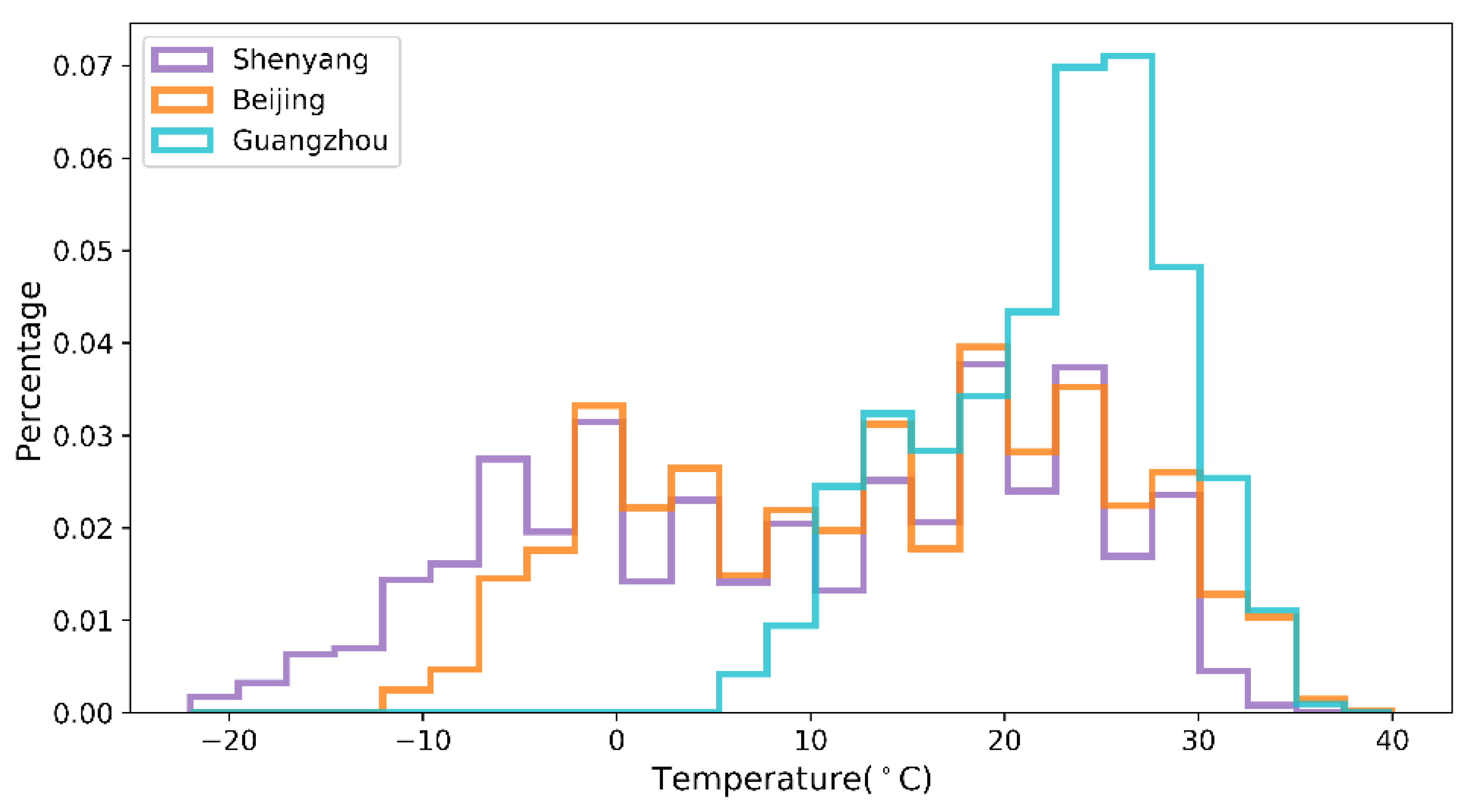
The temperature dataset records the temperature values for the three cities from 1 January 2015, at 00:00 h, to 31 December 2015, at 24:00 h, with a sampling frequency of 1 h for the sensors and a total of 24 datasets per day. The length of each dataset is 8760. The datasets are relatively complete, with only 1.3% of missing values (113 sets); the data are missing randomly, without continuous missing values. The missing values are filled and replaced using the average of two adjacent measurements. The temperature data of the three cities are shown in Figure 4. Shenyang and Beijing have four distinct seasons, while Guangzhou has more sunny and hotter weather. The lowest temperature in Shenyang in winter can reach −20 °C, while the lowest temperature in Guangzhou is only 5 °C. Moreover, the temperature fluctuation in Guangzhou is slight throughout the year, with a difference of 30 °C between the minimum and maximum temperatures, while the maximum temperature difference in Shenyang can reach 53 °C.

In December, most Chinese cities adopt greenhouse farming; 67% of these are plastic greenhouses. These plastic greenhouses do not have intelligent heating and ventilation equipment and rely entirely on physical methods, such as the laying out of insulation quilts, to control temperature. Temperature control in plastic greenhouses is heavily dependent on outdoor temperatures. Therefore, accurate prediction of the outdoor temperature is essential for greenhouse crop cultivation, and accurate temperature prediction can provide a basis for agricultural production planning to provide a suitable growing environment for crops in greenhouses. Therefore, we selected 8040 datasets from the first 11 months for model training and 720 datasets from December for testing.

The experiments in this paper use the root mean squared error (RMSE), mean absolute error (MAE), Pearson’s correlation coefficient (R), the symmetric mean absolute percentage error (SMAPE), the mean error (ME), and the standard deviation of errors (SDE) as evaluation model indicators. RMSE and MAE are standard error measures between the actual value and the forecast, while SMAPE is the deviation ratio, with smaller values indicating a closer match. The ME value is equal to or close to 0 for unbiased predictions. SDE measures the extent to which the error value deviates from the mean. R is used to measure the correlation between the predicted and actual values. The R value is close to 1, showing that the higher the correlation between the prediction and the ground truth, the better the model will fit. The formulas for these four metrics are shown below:

$$RMSE=\sqrt{\frac{1}{m}{\displaystyle \sum _{i=1}^m{\left(y_i-{\widehat{y}}_i\right)}^2}}$$

(28)

$$MAE=\frac{1}{m}{\displaystyle \sum _{i=1}^m\left|y_i-{\widehat{y}}_i\right|}$$

(29)

$$SMAPE=\frac{100\%}{m}{\displaystyle \sum _{i=1}^m\frac{\left|{\widehat{y}}_i-y_i\right|}{(\left|{\widehat{y}}_i\right|+\left|y_i\right|)/2}}$$

(30)

$$R=\frac{{\displaystyle {\sum }_{t=1}^T({\widehat{y}}_t-{\overline{\widehat{y}}}_t)(y_t-{\overline{y}}_t})}{\sqrt{{\displaystyle {\sum }_{t=1}^T(}{\widehat{y}}_t-{\overline{\widehat{y}}}_t{)}^2{\displaystyle {\sum }_{t=1}^T(y_t-}{\overline{y}}_t{)}^2}}$$

(31)

$$ME=\frac{1}{m}{\displaystyle \sum _{i=1}^m{\left({\widehat{y}}_i-y_i\right)}^{}}$$

(32)

$$SDE=\sqrt{\frac{1}{m-1}{\displaystyle \sum _{i=1}^m{\left(y_i-{\widehat{y}}_i\right)}^2}}$$

(33)

where $y_i$ is the ground truth value, ${\widehat{y}}_i$ is the prediction, $m$ represents the number of samples, $\overline{y_i}$ is the average of the ground truth value, and ${\overline{\widehat{y}}}_i$ is the average of the prediction.

4.2. Comparative Experiments

To verify the effectiveness of our proposed model, we selected nine deep-learning models for comparative experiments. The baseline models we used were the Linear, RNN, GRU, LSTM, Bi-LSTM, ESN, Encoder-Decoder, attention, and informer models.

Three cases were considered:

Case 1: 24 h of the past day was used to predict 24 h in the next day.

Case 2: 48 h of the past two days were used to predict 24 h in the next day.

Case 3: 48 h of the past two days were used to predict 48 h in the next two days.

The training parameters of the model were set as follows: the epoch was 200, the learning rate was 0.0001, and the optimizer was Adam. Other parameters are shown in

Table 1. Model parameters.

Parameters	Case 1	Case 2	Case 3
Batch size	12	24	48
Network layers	2	2	4
Hidden units	64	64	128
Encoder-decoder layers	1	1	2
Multi-head	2	2	2
ESN neuronal reservoir	400	800	1200

.

The BMAE-Net has many hyperparameters, among which the number of hidden layer units and batch size are the most sensitive hyperparameters and significantly impact the model performance. Other adjustable hyperparameters include epoch, dropout, the number of encoder/decoder layers, heads of multi-head attention, and optimizer. The detailed hyperparameter settings are shown in

Table 2. Bayesian optimization hyperparameter space and search results.

Parameters	Range	Case 1	Case 2	Case 3
Batch size	[6,50]	16	24	48
Network layers	[1,6]	1	2	3
Hidden units	[24,256]	36	72	120
Encoder/Decoder layers	[1,4]	1	2	2
Heads of multi-head attention	[1,3]	1	2	2
Epoch	[50,200]	65	110	135
Optimizer	[Adam, SGD, AdaGrad]	Adam	Adam	Adam

.

All models were written in a Python 3.8 environment, based on the PyTorch deep learning framework. All experiments were performed on a server with the following parameters: Ubuntu 20.04 64-bit operating system; Intel Core i7-6800K 3.4 GHz CPU; NVIDIA GTX 1080Ti 11G. The evaluation of model prediction performance is conducted using the evaluation metrics mentioned in Section 4.1.

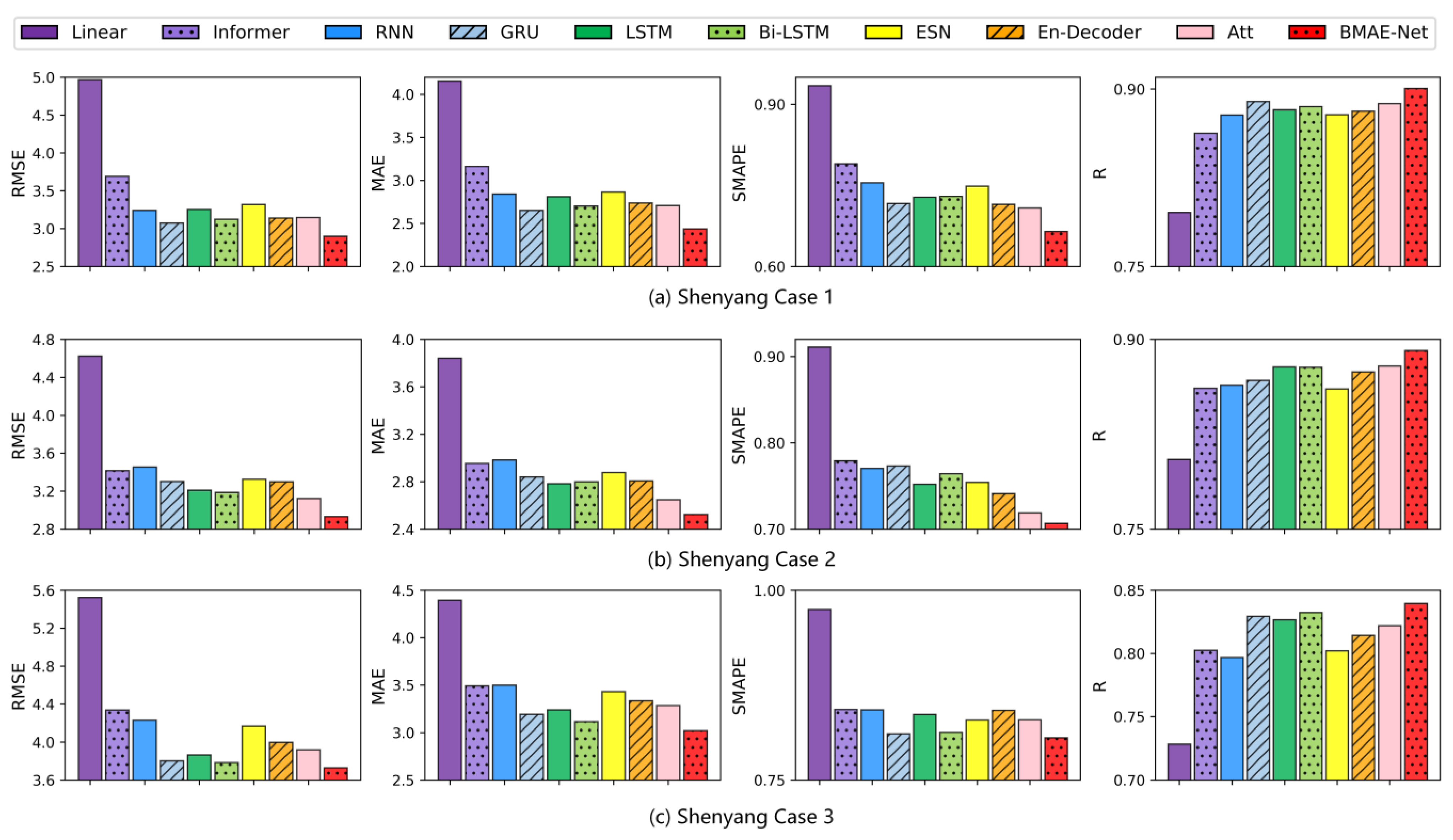
The results of temperature experiments in the Shenyang area are shown in

Table 3. Experimental results for temperature from the Shenyang station.

Step	Case 1				Case 2				Case 3
Metric	RMSE	MAE	SMAPE	R	RMSE	MAE	SMAPE	R	RMSE	MAE	SMAPE	R
Linear	4.966	4.153	0.934	0.796	4.623	3.840	0.911	0.805	5.523	4.395	0.975	0.728
Informer	3.692	3.161	0.790	0.863	3.416	2.953	0.779	0.861	4.336	3.491	0.843	0.802
RNN	3.240	2.842	0.755	0.878	3.454	2.982	0.770	0.864	4.228	3.498	0.842	0.797
GRU	3.073	2.652	0.716	0.889	3.302	2.840	0.773	0.868	3.803	3.190	0.811	0.829
LSTM	3.254	2.811	0.728	0.883	3.210	2.783	0.752	0.878	3.865	3.237	0.836	0.827
Bi-LSTM	3.122	2.701	0.730	0.885	3.186	2.798	0.764	0.878	3.784	3.113	0.813	0.832
ESN	3.318	2.864	0.748	0.878	3.326	2.876	0.754	0.861	4.167	3.429	0.829	0.802
Encoder-Decoder	3.138	2.738	0.715	0.881	3.298	2.805	0.741	0.874	3.996	3.333	0.841	0.814
Attention	3.146	2.707	0.708	0.888	3.122	2.648	0.719	0.879	3.919	3.283	0.829	0.822
BMAE-Net	2.899	2.437	0.665	0.900	2.933	2.523	0.707	0.891	3.728	3.022	0.806	0.840

. As seen from Table 3 and Figure 5, the RMSE, MAE, and SMAPE indicators of the model proposed in this paper are lower than those of the other baseline models, which indicates that the model has the smallest difference between the prediction and the ground truth. The R indicators are greater than the other models, meaning that the BMAE-Net model has the highest goodness of fit. In Case 1, the RMSE, MAE, and SMAPE of the BMAE-Net model were 5.7%, 8.1%, and 7.2% lower than the GRU model, which was the best-performing model on this dataset, and the R indicator was 1.2% higher. In Case 2, compared to the attention model, which was the best-performing model on this dataset, the BMAE-Net model’s RMSE, MAE, and SMAPE were 6.1%, 4.7%, and 1.7% lower than the attention model, and the R metric improved by 1.4%. In Case 3, compared to the best-performing Bi-LSTM model on this dataset, the BMAE-Net model’s RMSE, MAE, and SMAPE were 1.5%, 2.9%, and 0.9%, and the R metric improved by 0.9%.

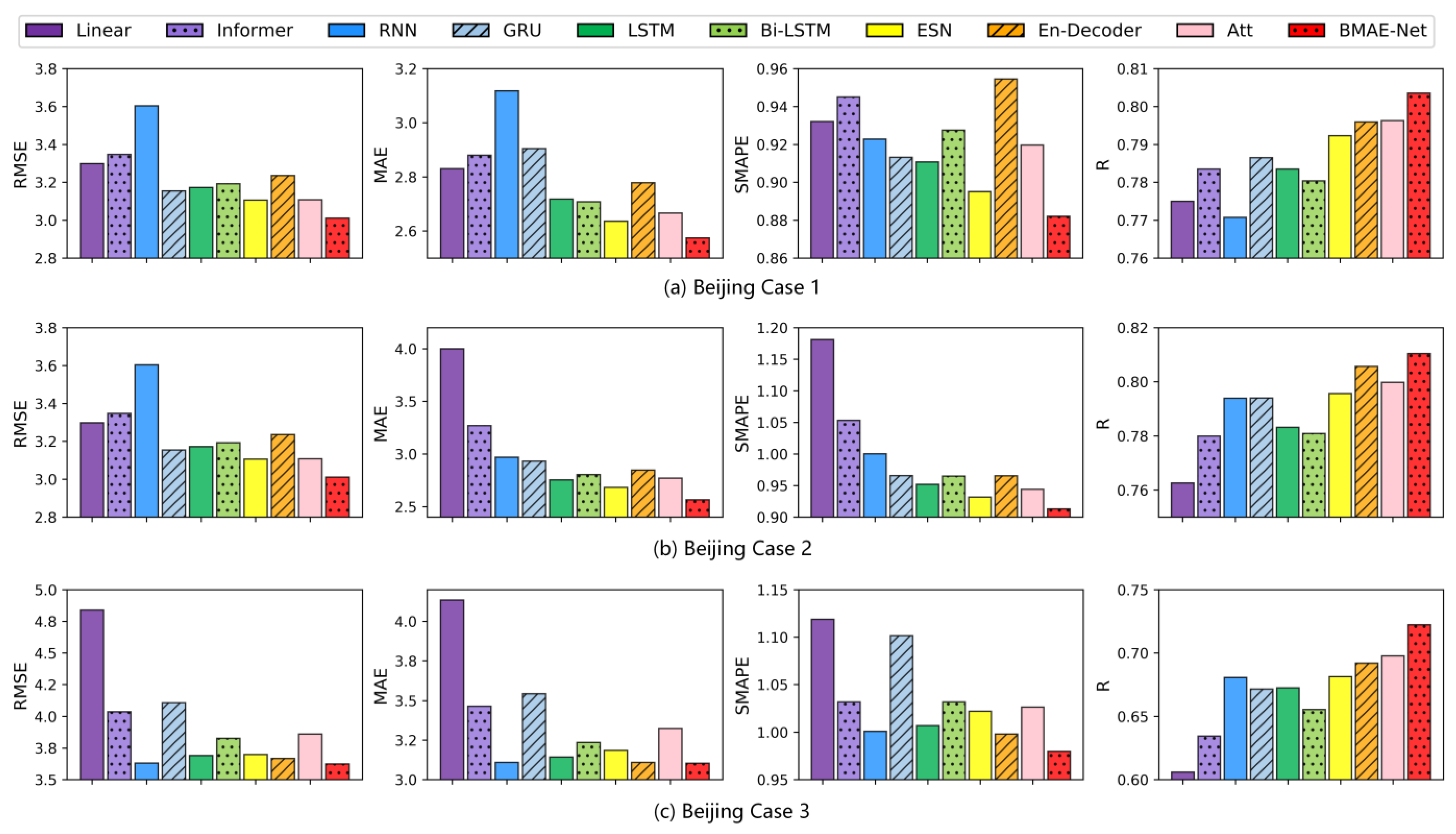
The results of the temperature experiments in the Beijing area are shown in

Table 4. Experimental results for temperature from the Beijing station.

Step	Case 1				Case 2				Case 3
Metric	RMSE	MAE	SMAPE	R	RMSE	MAE	SMAPE	R	RMSE	MAE	SMAPE	R
Linear	3.299	2.830	0.932	0.775	4.404	4.000	1.181	0.763	4.840	4.134	1.119	0.606
Informer	3.347	2.880	0.945	0.784	3.691	3.269	1.053	0.780	4.037	3.464	1.032	0.634
RNN	3.604	3.118	0.923	0.771	3.415	2.968	1.000	0.794	3.630	3.108	1.001	0.681
GRU	3.154	2.905	0.913	0.786	3.394	2.931	0.966	0.794	4.109	3.542	1.101	0.671
LSTM	3.172	2.718	0.911	0.783	3.189	2.753	0.952	0.783	3.690	3.142	1.007	0.672
Bi-LSTM	3.193	2.708	0.928	0.780	3.257	2.805	0.965	0.781	3.826	3.235	1.032	0.655
ESN	3.106	2.636	0.895	0.792	3.110	2.683	0.932	0.796	3.699	3.186	1.022	0.681
Encoder-Decoder	3.235	2.778	0.954	0.796	3.276	2.847	0.966	0.806	3.667	3.108	0.998	0.692
Attention	3.108	2.666	0.920	0.796	3.204	2.771	0.944	0.800	3.860	3.324	1.026	0.698
BMAE-Net	3.011	2.574	0.882	0.804	3.000	2.576	0.926	0.810	3.624	3.104	0.980	0.722

. As can be seen from Table 4 and Figure 6, the RMSE, MAE, and SMAPE indicators of the model proposed are lower than the other baseline models, which indicates that the model exhibits the smallest difference between the prediction and the ground truth. The R indicators are greater than in the other models, indicating that the model has the highest goodness of fit.

In Case 1, the BMAE-Net model had 3.1%, 2.4%, and 1.5% lower RMSE, MAE, and SMAPE values and a 1.4% higher R-indicator compared to the ESN model that performed best on this dataset. In Case 2, the BMAE-Net model had lower RMSE, MAE, and SMAPE values, which decreased by 4.1%, 4.4%, and 2% compared to the ESN model, and the R metric improved by 1.9%. In Case 3, the RMSE, MAE, and SMAPE of the BMAE-Net model decreased by 1%, 0.2%, and 1.8% compared to the encoder-decoder model, which was the best-performing model on this dataset, and the R indicators improved by 4.4%.

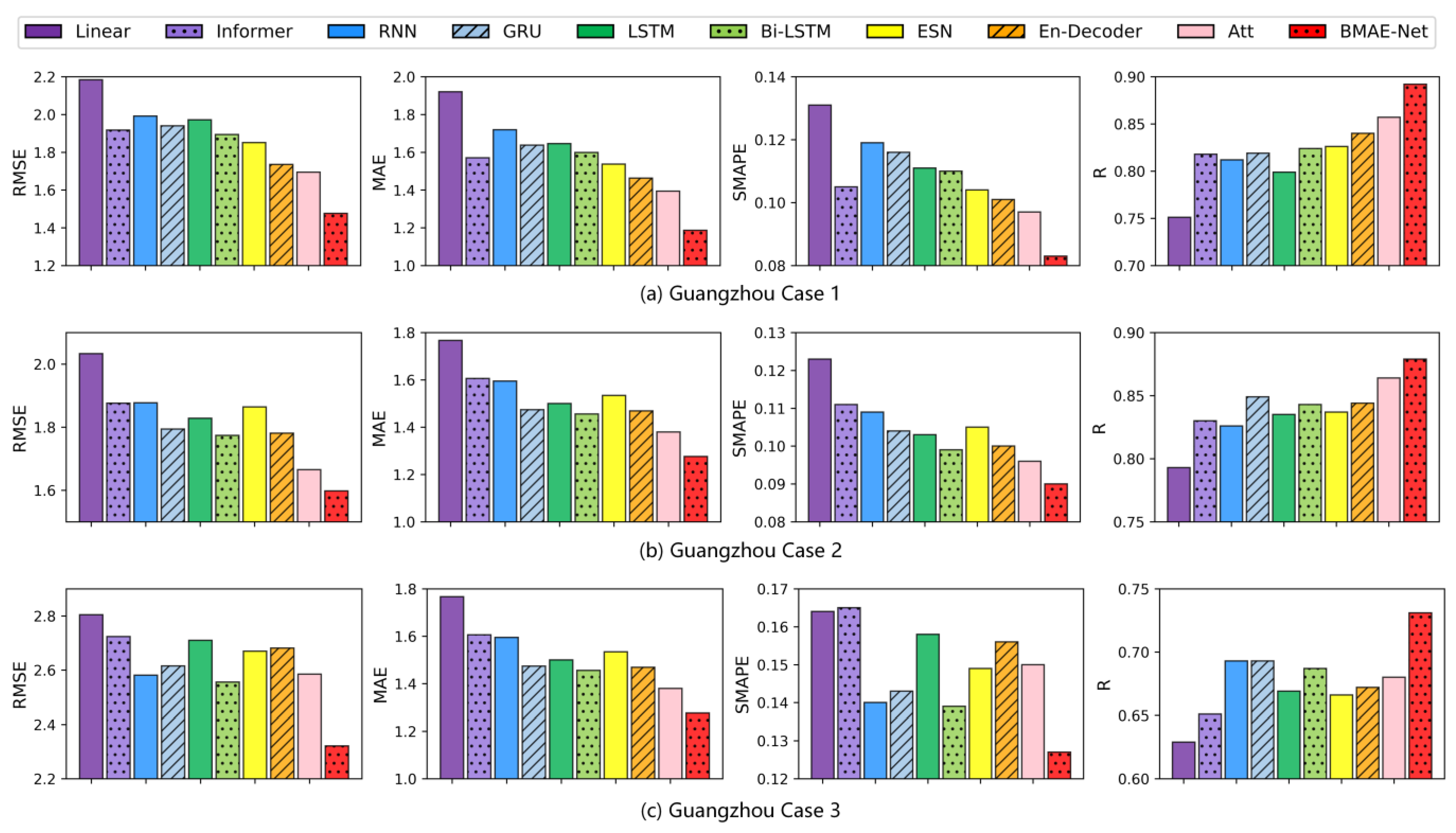
The results of the temperature experiments in the Guangzhou area are shown in

Table 5. Experimental results for temperature from the Guangzhou station.

Step	Case 1				Case 2				Case 3
Metric	RMSE	MAE	SMAPE	R	RMSE	MAE	SMAPE	R	RMSE	MAE	SMAPE	R
Linear	2.184	1.920	0.131	0.751	2.033	1.767	0.123	0.793	2.804	2.414	0.164	0.629
Informer	1.917	1.571	0.105	0.818	1.876	1.606	0.111	0.830	2.724	2.392	0.165	0.651
RNN	1.992	1.719	0.119	0.812	1.877	1.595	0.109	0.826	2.581	2.121	0.140	0.693
GRU	1.940	1.638	0.116	0.819	1.794	1.474	0.104	0.849	2.615	2.163	0.143	0.693
LSTM	1.972	1.646	0.111	0.799	1.828	1.500	0.103	0.835	2.710	2.335	0.158	0.669
Bi-LSTM	1.894	1.599	0.110	0.824	1.774	1.456	0.099	0.843	2.556	2.113	0.139	0.687
ESN	1.851	1.537	0.104	0.826	1.864	1.534	0.105	0.837	2.670	2.232	0.149	0.666
Encoder-Decoder	1.735	1.463	0.101	0.840	1.781	1.469	0.100	0.844	2.681	2.307	0.156	0.672
Attention	1.695	1.394	0.097	0.857	1.665	1.380	0.096	0.864	2.585	2.227	0.150	0.680
BMAE-Net	1.476	1.187	0.083	0.892	1.598	1.276	0.090	0.879	2.321	1.921	0.127	0.731

. As seen from Table 5 and Figure 7, the RMSE, MAE, and SMAPE metrics of the model proposed in this paper are lower than those of the other baseline models, which indicates that the model has a minor difference between the prediction and the ground truth. The R metrics are greater than those of the other models, meaning that the model has the best fit. In Case 1, the BMAE-Net model had 13%, 15%, and 14.4% lower RMSE, MAE, and SMAPE values and a 4.1% higher R-indicator than the attention model, compared to the best-performing attention model on this dataset. In Case 2, compared to the best-performing attention model on this dataset, the BMAE-Net model had 4%, 7.5%, and 6.3% lower RMSE, MAE, and SMAPE values and 1.7% better R metrics than the attention model. In Case 3, compared to the best-performing Bi-LSTM model on this dataset, the BMAE-Net model had 9%, 9%, and 8.6% lower RMSE, MAE, and SMAPE values than the Bi-LSTM model, and the R metric improved by 6.4%.

4.3. Ablation Experiments

In order to validate the Bayesian encoder-decoder model based on the attention mechanism proposed in this paper, the modeling predictions were validated using the temperature data from three cities. The same arrangement used in the comparison experiments in Section 4.2 was employed to set up MHAtt, BLinear, BLSTM, BGRU, and BMED-Net, to compare the prediction results for the three cases.

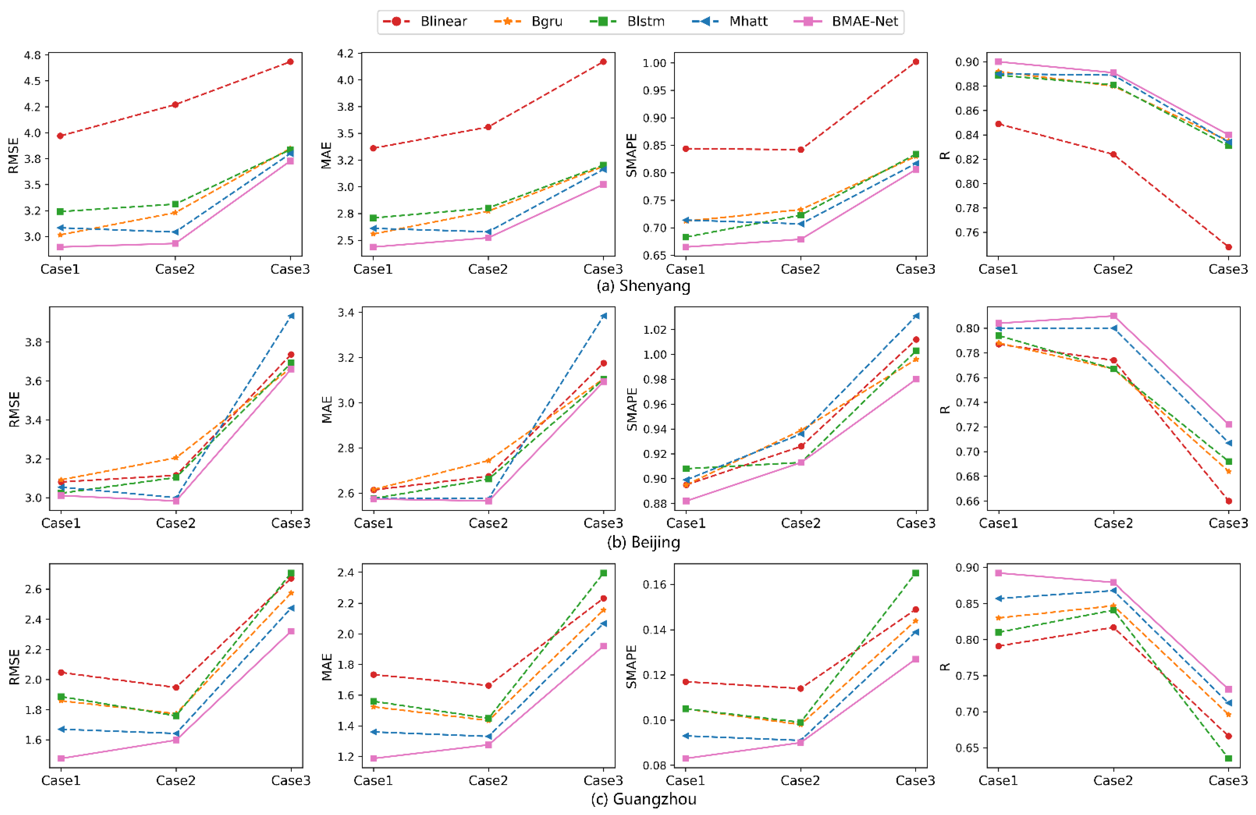
As seen from

Table 6. The experimental results for temperature for each location.

Location	Step	Metric	BMAE-Net	BLinear	BGRU	BLSTM	MHatt
Shenyang	Case 1	RMSE	2.899	3.969	3.016	3.240	3.084
		MAE	2.437	3.360	2.558	2.708	2.611
		SMAPE	0.665	0.844	0.712	0.683	0.714
		R	0.900	0.849	0.892	0.889	0.890
	Case 2	RMSE	2.933	4.271	3.230	3.312	3.043
		MAE	2.523	3.559	2.772	2.802	2.579
		SMAPE	0.679	0.842	0.733	0.723	0.707
		R	0.891	0.824	0.880	0.881	0.889
	Case 3	RMSE	3.728	4.684	3.849	3.837	3.799
		MAE	3.022	4.169	3.191	3.203	3.162
		SMAPE	0.806	1.002	0.830	0.834	0.817
		R	0.840	0.748	0.835	0.831	0.834
Beijing	Case 1	RMSE	3.011	3.081	3.092	3.023	3.054
		MAE	2.574	2.614	2.616	2.576	2.576
		SMAPE	0.882	0.895	0.895	0.908	0.899
		R	0.804	0.787	0.788	0.794	0.800
	Case 2	RMSE	2.983	3.115	3.205	3.104	3.000
		MAE	2.565	2.675	2.744	2.662	2.576
		SMAPE	0.913	0.926	0.939	0.913	0.936
		R	0.810	0.774	0.767	0.767	0.800
	Case 3	RMSE	3.660	3.736	3.667	3.692	3.934
		MAE	3.093	3.175	3.106	3.104	3.384
		SMAPE	0.980	1.012	0.996	1.003	1.031
		R	0.722	0.660	0.684	0.692	0.707
Guangzhou	Case 1	RMSE	1.476	2.047	1.859	1.887	1.670
		MAE	1.187	1.734	1.524	1.560	1.360
		SMAPE	0.083	0.117	0.105	0.105	0.093
		R	0.892	0.791	0.830	0.810	0.857
	Case 2	RMSE	1.598	1.947	1.773	1.759	1.642
		MAE	1.276	1.663	1.435	1.449	1.331
		SMAPE	0.090	0.114	0.098	0.099	0.091
		R	0.879	0.817	0.847	0.841	0.868
	Case 3	RMSE	2.321	2.670	2.574	2.705	2.474
		MAE	1.921	2.232	2.155	2.395	2.068
		SMAPE	0.127	0.149	0.144	0.165	0.139
		R	0.731	0.666	0.696	0.635	0.712

and Figure 8, in the temperature prediction experiments in each location, compared with the MHAtt model, the BMAE-Net model that incorporated variational inference improved in all evaluation indexes, and the model prediction was better. Meanwhile, the model results for BLinear, BGRU, and BLSTM were also better than those for Linear, GRU, and LSTM, which indicates that with the inclusion of variational inference, the fitting ability of the model was improved, and better prediction could be achieved.

In order to see the magnitude of each metric more clearly, a line graph of the evaluation metrics of each compared model was plotted. As seen from Figure 8, for nonlinear time series data with sensor measurement errors and severe interference from the external environment, the proposed multi-head attention encoder-decoder neural network, optimized via a Bayesian inference strategy, has the advantages of higher accuracy and better generalization than other prediction models.

We selected four comparison models to calculate the ME and SDE values. The closer the value for ME is to 0, the smaller the model error is, while a value for ME of less than 0 indicates that the overall predicted value is smaller than the ground truth value, and a value greater than 0 is the opposite. The smaller the SDE, the smaller the error deviation from the mean, and vice versa.

Table 7. The model parameters.

Case 1	Shenyang		Beijing		Guangzhou
Metrics	ME	SDE	ME	SDE	ME	SDE
GRU	0.2482	3.5019	1.3105	3.4355	−0.2278	2.1746
Bi-LSTM	0.1959	3.5374	0.7520	3.4569	−0.1447	2.1123
Encoder-Decoder	0.3975	3.6614	1.3210	3.5164	−0.0157	1.9279
Attention	−0.3309	3.4998	0.7489	3.4306	0.0044	1.8782
BMAE-Net	−0.1170	3.2593	0.5610	3.3730	0.0307	1.6193

shows that the proposed model has lower ME and SDE values than other baselines in Case 1, proving that BMAE-Net has better prediction performance.

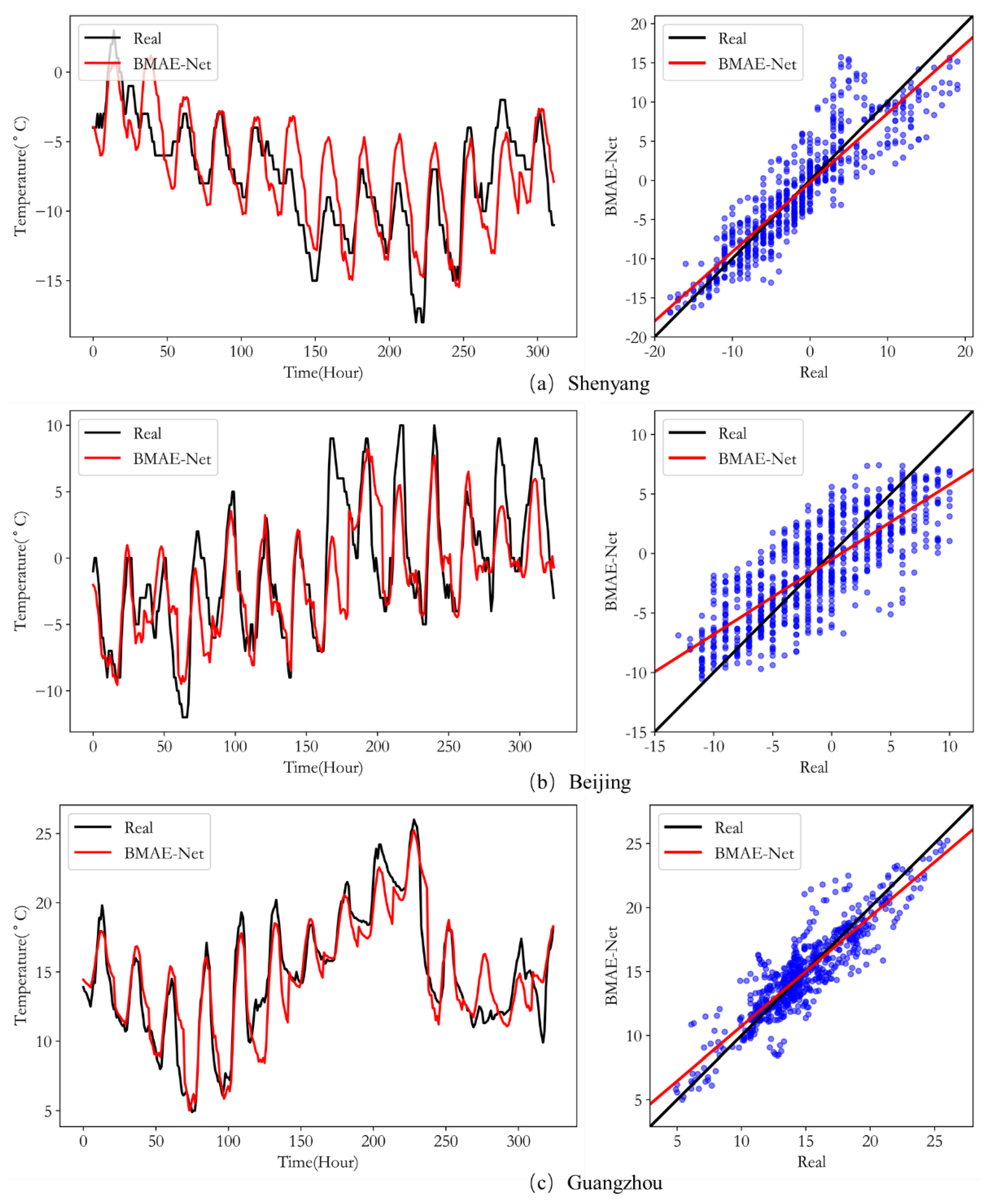
Figure 9 plots the curves of the predicted and ground truth values (left) and the scatter plot (right) for our model in the test for Case 1. The x-axis of the fit plot is time, while the y-axis is temperature. The more the curves of the ground truth and predicted values repeat, the closer the predicted values are to the ground truth values. As shown in each subplot on the left of Figure 9, the model can predict the temperature trend in Case 1; the model works best on the Guangzhou dataset, followed by Shenyang. This is because Guangzhou has a relatively concentrated temperature distribution throughout the year, while Shenyang and Beijing have cold winters in December and undergo large temperature changes in the morning and evening, so the temperature dataset is more of a challenge to fit. The scatter plot is drawn using the linear regression model of the predicted and ground truth values; the x-axis is the ground truth value, the y-axis is the predicted value, the black line is the linear regression of the ground truth value, and the red line is the prediction model. The closer the two lines are, the closer the predicted value is to the ground truth value; the closer the blue points in the plot are to the black line, the higher the correlation between the predicted and ground truth values. As shown by the subplots in Figure 9, the predicted and ground truth values are strongly correlated, which is especially evident in the Guangzhou data, where the predicted values are concentrated around the regression line, indicating that our model performs well on the temperature prediction task. In summary, the experimental results demonstrate that the model has excellent multi-step prediction performance under different datasets.

4.4. Discussion

In the comparison experiments, we performed three cases of effect validation on the temperature datasets of three locations separately. The experimental results are shown in the first two subsections; in most cases, the BMAE-Net error designed in this paper is smaller than the remaining nine comparison models, and the fit is better than the comparison models. For example, the R evaluation metrics for temperature prediction in the three locations are 0.9, 0.804, and 0.892, respectively, while the RMSE is reduced to 2.899, 3.011, and 1.476 in the Case 1 temperature data. Among the prediction performances of the three locations, the best results were obtained for the Guangzhou site, which we speculate is because the temperature data distribution in Guangzhou is more concentrated, while the temperature data distribution in Shenyang and Beijing is more dispersed (as shown in Figure 4), which indicates that the quality of the dataset also has an impact on the model performance.

In the ablation experiments, we incorporated Bayesian mechanisms for the Linear, GRU, LSTM, and multi-headed attention models, respectively, so that the internal parameters conformed to a normal distribution and the weights and biases were continuously corrected to achieve optimal results when backpropagating. Ablation experiments further confirmed that including variational inference improved the R-evaluation metrics of the model, while reducing each error evaluation metric. From the experimental results, it can be concluded that BLinear, BLSTM, BGRU, and BMAE-Net all outperformed the model without incorporating Bayesian principles, proving that the introduction of the Bayesian principle contributes to the model’s performance and can improve its predictive power.

The BMAE-Net model in this paper is based on Bayesian principles for parameter optimization to establish the optimal parameters. The model is continuously trained to establish the optimal parameters within our preset parameter range. The process of finding the optimal parameters was long, and we noted the time needed for the Bayesian optimization process during the experiments. When the Case 1 experiment was conducted, the average training time for the three locations was 17 h 23 min. At the same time, the other comparison models were trained according to our preset parameters, and the usual training time was about 8 min 35 s. It can be seen that the time cost of Bayesian optimization was higher, and the parameters generated during the training process became elevated. However, compared with parameter optimization methods, such as grid and random searches, the time needed has been reduced significantly.

5. Conclusions

Temperature, an essential factor on which crop production depends, affects crop growth, development, and yield. Accurate temperature prediction can guide farming operations. In this paper, a Bayesian optimization-based multi-head attention encoder-decoder model is proposed to implement the prediction of weather parameters. A holistic encoder-decoder framework is used, with Bayesian-GRUs as the basic units of the encoder and decoder, combined with a multi-head attention structure based on variational inference. The model is validated on temperature data from three locations and has better generalization performance and robustness than other baseline models with different prediction forecasting steps. The best performance can be demonstrated on meteorological data with strong nonlinear characteristics and data with errors, and the intrinsic characteristics of the data can be fully explored and predicted. Eventually, the model can achieve a 24-hour accurate temperature prediction to provide a guiding basis for agricultural production planning and a suitable growing environment for crops.

In subsequent work, the model will be further optimized, and its application will be extended to other types of time series data. Meanwhile, the introduction of Bayesian optimization inevitably increases the computational cost and requires more training time; therefore, the model will be optimized in terms of computational cost in the next step.

References

1. Liu, Y.; Li, D.; Wan, S. A long short-term memory-based model for greenhouse climate prediction. Int. J. Intell. Syst. 2022, 37, 135–151. [Google Scholar] [CrossRef]
2. Schultz, M.G.; Betancourt, C.; Gong, B.; Kleinert, F.; Langguth, M.; Leufen, L.H.; Mozaffari, A.; Stadtler, S. Can deep learning beat numerical weather prediction? Philos. Trans. R. Soc. A 2021, 379, 2194. [Google Scholar] [CrossRef]
3. Jin, X.-B.; Wang, Z.-Y.; Kong, J.-L.; Bai, Y.-T.; Su, T.-L.; Ma, H.-J.; Chakrabarti, P. Deep spatio-temporal graph network with self-optimization for air quality prediction. Entropy 2023, 25, 247. [Google Scholar] [CrossRef]
4. Chen, J.-H.; Lin, S.-J.; Magnusson, L.; Bender, M.; Chen, X.; Zhou, L. Advancements in hurricane prediction with NOAA’s next-generation forecast system. Geophys. Res. Lett. 2019, 46, 4495–4501. [Google Scholar] [CrossRef] [Green Version]
5. Manogaran, G.; Hsu, C.H.; Rawal, B.S.; Muthu, B.; Mavromoustakis, C.X.; Mastorakis, G. ISOF: Information scheduling and optimization framework for improving the performance of agriculture systems aided by industry 4.0. IEEE Internet Things J. 2022, 8, 3120–3129. [Google Scholar] [CrossRef]
6. Klem, K.; Váňová, M.; Hajšlová, J.; Lancová, K.; Sehnalová, M. A neural network model for prediction of deoxynivalenol content in wheat grain based on weather data and preceding crop. Plant Soil Environ. 2007, 53, 421–429. [Google Scholar] [CrossRef] [Green Version]
7. Ferreira, P.M.; FariaE, A.; RuanoA, E. Neural network models in greenhouse air temperature prediction. Neurocomputing 2002, 43, 51–75. [Google Scholar] [CrossRef] [Green Version]
8. Kong, J.; Yang, C.; Wang, J.; Wang, X.; Zuo, M.; Jin, X.; Lin, S. Deep-stacking network approach by multisource data mining for hazardous risk identification in IoT-based intelligent food management systems. Comput. Intell. Neurosci. 2021, 2021, 1194565. [Google Scholar] [CrossRef]
9. Fourati, F.; Chtourou, M. A greenhouse control with feed-forward and recurrent neural networks. Simul. Model. Pract. Theory 2007, 15, 1016–1028. [Google Scholar] [CrossRef]
10. Xia, D.; Wang, B.; Li, H.; Li, Y.; Zhang, Z. A distributed spatial–temporal weighted model on MapReduce for short-term traffic flow forecasting. Neurocomputing 2016, 179, 246–263. [Google Scholar] [CrossRef]
11. Jin, X.B.; Yu, X.H.; Wang, X.Y.; Bai, Y.T.; Su, T.L.; Kong, J.L. Deep learning predictor for sustainable precision agriculture based on internet of things system. Sustainability 2020, 12, 1433. [Google Scholar] [CrossRef] [Green Version]
12. Kong, J.L.; Wang, H.X.; Wang, X.Y.; Jin, X.B.; Fang, X.; Lin, S. Multi-stream hybrid architecture based on cross-level fusion strategy for fine-grained crop species recognition in precision agriculture. Comput. Electron. Agric. 2021, 185, 106134. [Google Scholar] [CrossRef]
13. Fu, T. A review on time series data mining. Eng. Appl. Artif. Intell. 2011, 24, 164–181. [Google Scholar] [CrossRef]
14. Kong, J.; Wang, H.; Yang, C.; Jin, X.; Zuo, M.; Zhang, X. A spatial feature-enhanced attention neural network with high-order pooling representation for application in pest and disease recognition. Agriculture 2022, 12, 500. [Google Scholar] [CrossRef]
15. Zheng, Y.Y.; Kong, J.L.; Jin, X.B.; Wang, X.Y.; Zuo, M. CropDeep: The crop vision dataset for deep-learning-based classification and detection in precision agriculture. Sensors 2019, 19, 1058. [Google Scholar] [CrossRef] [Green Version]
16. Katris, C. A time series-based statistical approach for outbreak spread forecasting: Application of COVID-19 in Greece. Expert Syst. Appl. 2020, 166, 114077. [Google Scholar] [CrossRef]
17. Ebadi, A.; Xi, P.; Tremblay, S. Understanding the temporal evolution of COVID-19 research through machine learning and natural language processing. Scientometrics 2021, 126, 725–739. [Google Scholar] [CrossRef]
18. Li, J.; Sun, L.; Yan, Q.; Li, Z.; Srisa, A.-W.; Ye, H. Significant permission identification for machine-learning- based android malware detection. IEEE Trans. Ind. Inform. 2018, 14, 3216–3225. [Google Scholar] [CrossRef]
19. Zeng, M.; Li, S.L.; Wang, L.; Xue, S.; Wang, R.C. Wind power prediction model based on the combined optimization algorithm of ARMA model and BP neural networks. East China Electric Power 2013, 41, 347–352. [Google Scholar]
20. Wang, Y.; Wang, C.; Shi, C. Short-term cloud coverage prediction using the ARIMA time series model. Remote Sens. Lett. 2018, 9, 275–284. [Google Scholar] [CrossRef]
21. Chen, H. A new load forecasting method based on generalized autoregressive conditional heteroscedasticity model. Autom. Electr. Power Syst. 2007, 31, 51–54. [Google Scholar]
22. Xiao, Z.; Ye, S.J.; Zhong, B.; Sun, C.X. BP neural network with rough set for short term load forecasting. Expert Syst. Appl. 2009, 36, 273–279. [Google Scholar] [CrossRef]
23. Moon, J.; Kim, Y.; Son, M.; Hwang, E. Hybrid short-term load forecasting scheme using random forest and multilayer perceptron. Energies 2018, 11, 3283. [Google Scholar] [CrossRef] [Green Version]
24. Yu, H.; Chen, Y.; Hassan, S.G.; Li, D. Prediction of the temperature in a Chinese solar greenhouse based on LSSVM optimized by improved PSO. Comput. Electron. Agric. 2016, 122, 94–102. [Google Scholar] [CrossRef]
25. Zhu, S.; Luo, X.; Chen, S.; Xu, Z.; Xiao, Z. Improved hidden Markov model incorporated with copula for probabilistic seasonal drought forecasting. J. Hydrol. Eng. 2020, 25, 04020019. [Google Scholar] [CrossRef]
26. Kong, J.; Yang, C.; Lin, J.; Xiao, Y.; Lin, S.; Ma, K.; Zhu, Q. A graph-related high-order neural network architecture via feature aggregation enhancement for identification application of diseases and pests. Comput. Intel. Neurosc. 2022, 2022, 4391491. [Google Scholar] [CrossRef]
27. Jin, X.; Zhang, J.; Kong, J.; Su, T.; Bai, Y. A reversible automatic selection normalization (RASN) deep network for predicting in the smart agriculture system. Agronomy 2022, 12, 591. [Google Scholar] [CrossRef]
28. Li, Q.; Zhu, Y.; Wei, S.; Wang, X.; Li, L.; Yu, F. An attention-aware LSTM model for soil moisture and soil temperature prediction. Geoderma 2022, 409, 115651. [Google Scholar] [CrossRef]
29. Jin, X.-B.; Yang, N.-X.; Wang, X.-Y.; Bai, Y.-T.; Su, T.-L.; Kong, J.-L. Hybrid deep learning predictor for smart agriculture sensing based on empirical mode decomposition and gated recurrent unit group model. Sensors 2020, 20, 1334. [Google Scholar] [CrossRef] [Green Version]
30. Sehovac, L.; Grolinger, K. Deep learning for load forecasting: Sequence to sequence recurrent neural networks with attention. IEEE Access 2020, 8, 36411–36426. [Google Scholar] [CrossRef]
31. Kao, I.; Zhou, Y.; Chang, L.; Chang, L. Exploring a long short-term memory based encoder-decoder framework for multi-step-ahead flood forecasting. J. Hydrol. 2020, 583, 124631. [Google Scholar] [CrossRef]
32. Baniata, L.H.; Park, S.; Park, S.B. A neural machine translation model for arabic dialects that utilizes multitask learning. Comput. Intel. Neurosc. 2018, 2018, 1–10. [Google Scholar] [CrossRef]
33. Xiao, X.; Wang, L.; Ding, K. Deep hierarchical encoder–decoder network for image captioning. IEEE Trans. Multimedia 2019, 21, 2942–2956. [Google Scholar] [CrossRef]
34. Du, S.; Li, T.; Yang, Y.; Shi, J.H. Multivariate time series forecasting via attention-based encoder-decoder framework. Neurocomputing 2020, 388, 269–279. [Google Scholar] [CrossRef]
35. Jin, X.B.; Zheng, W.Z.; Kong, J.L.; Wang, X.Y.; Zuo, M.; Zhang, Q.C.; Lin, S. Deep-learning temporal predictor via bi-directional self-attentive encoder decoder framework for IOT-based environmental sensing in intelligent greenhouse. Agriculture 2021, 11, 802. [Google Scholar] [CrossRef]
36. Nandi, A.; Arkadeep, D.; Mallick, A.; Middya, A.I.; Roy, S. Attention based long-term air temperature forecasting network: ALTF Net. Knowl. Based Syst. 2022, 252, 109442. [Google Scholar] [CrossRef]
37. Vaswani, A.; Shazeer, N.; Parmar, N. Attention is all you need. In Proceedings of the Thirty-First Annual Conference on Neural Information Processing Systems, Long Beach, CA, USA, 4–9 December 2017; pp. 5998–6008. [Google Scholar]
38. Kitaev, N.; Kaiser, U.; Levskaya, A. Reformer: The efficient transformer. In Proceedings of the International Conference on Learning Representations, Onlline, 27–30 April 2020. [Google Scholar]
39. Zhou, H.; Zhang, S.; Peng, J.; Zhang, S.; Li, J.; Xiong, H.; Zhang, W. Informer: Beyond efficient transformer for long sequence time-series forecasting. In Proceedings of the Association for the Advancement of Artificial Intelligence, Online, 2–9 February 2021. [Google Scholar]
40. Li, S.; Jin, X.; Xuan, Y.; Zhou, X.; Chen, W.; Wang, Y.X.; Yan, X. Enhancing the locality and breaking the memory bottleneck of transformer on time series forecasting. In Proceedings of the Neural Information Processing Systems, Vancouver, BC, Canada, 8–14 December 2019; pp. 5244–5254. [Google Scholar]
41. Goan, E.; Fookes, C. Bayesian neural networks: An introduction and survey. In Case Studies in Applied Bayesian Data Science; Mengersen, K., Pudlo, P., Robert, C., Eds.; Springer: Cham, Switzerland, 2020; Volume 1, pp. 45–87. [Google Scholar]
42. Song, M.; Cho, Y. Modeling maximum tsunami heights using bayesian neural networks. Atmosphere 2020, 11, 1266. [Google Scholar] [CrossRef]
43. Jin, X.B.; Wang, Z.Y.; Gong, W.T.; Kong, J.L.; Bai, Y.T.; Su, T.L.; Ma, H.J.; Chakrabarti, P. Variational Bayesian Network with Information Interpretability Filtering for Air Quality Forecasting. Mathematics 2023, 11, 837. [Google Scholar] [CrossRef]
44. Osawa, K.; Swaroop, S.; Jain, A.; Eschenhagen, R.; Turner, R.E.; Yokota, R. Practical deep learning with bayesian principles. NIPS 2019, 33, 4287–4299. [Google Scholar]
45. Steinbrener, J.; Posch, K.; Pilz, J. Measuring the uncertainty of predictions in deep neural networks with variational inference. Sensors 2020, 20, 6011. [Google Scholar] [CrossRef]
46. Jin, X.B.; Gong, W.T.; Kong, J.L.; Bai, Y.T.; Su, T.L. PFVAE: A planar flow-based variational auto-encoder prediction model for time series data. Mathematics 2022, 10, 610. [Google Scholar] [CrossRef]
47. Park, D.; Yoon, S. A missing value replacement method for agricultural meteorological data using bayesian spatio–temporal model. J. Environ. Sci. Int. 2018, 27, 499–507. [Google Scholar] [CrossRef]
48. Jiang, B.; Gong, H.; Qin, H.; Zhu, M. Attention-LSTM architecture combined with Bayesian hyperparameter optimization for indoor temperature prediction. Build. Environ. 2022, 224, 109536. [Google Scholar] [CrossRef]
49. Cho, H.; Kim, Y.; Lee, E.; Choi, D.; Lee, Y.; Rhee, W. Basic enhancement strategies when using bayesian optimization for hyperparameter tuning of deep neural networks. IEEE Access 2020, 8, 52588–52608. [Google Scholar] [CrossRef]
50. Kolar, D.; Lisjak, D.; Pająk, M.; Gudlin, M. Intelligent fault diagnosis of rotary machinery by convolutional neural network with automatic hyper-parameters tuning using bayesian optimization. Sensors 2021, 21, 2411. [Google Scholar] [CrossRef]
51. Dairy, B.; Valverde, J.; Moura, M.F.; Lopes, A. A survey of the applications of bayesian networks in agriculture. Eng. Appl. Artif. Intel. 2017, 65, 29–42. [Google Scholar]
52. Cho, K.; Merrienboer, B.; Gulcehre, C.; Bahdanau, D.; Bougares, F.; Schwenk, H.; Bengio, Y. Learning phrase representations using RNN encoder–decoder for statistical machine translation. In Proceedings of the 2014 Conference on Empirical Methods in Natural Language Processing, Doha, Qatar, 25–29 October 2014; pp. 1724–1734. [Google Scholar]
Figure 1. The overall framework of the BMAE-Net.
Agronomy 13 00625 g001
Figure 2. Bayesian-GRU structure. The blue box in the figure shows our proposed Bayesian-GRU module, the pink box shows the input temperature data, x t , and the output, y t , predicted by the model, and the blue circle, h t , shows the hidden state information at the current moment. W t and b t are the weights and biases within the GRU, which we incorporated into the Bayesian variational inference (as shown in the green box). W t and b t are no longer specific values; we transformed them by translation and scaling, using a Gaussian distribution with mean μ and standard deviation σ .
Agronomy 13 00625 g002
Figure 3. Bayesian multi-head-attention structure.
Agronomy 13 00625 g003
Figure 4. Histograms of the air temperature measurement datasets from three locations, used for model training and validation.
Agronomy 13 00625 g004
Figure 5. Bar graph of the temperature forecast evaluation index for the Shenyang station.
Agronomy 13 00625 g005
Figure 6. Bar graph of the temperature forecast evaluation index for the Beijing station.
Agronomy 13 00625 g006
Figure 7. Bar graph of the temperature forecast evaluation index for the Guangzhou station.
Agronomy 13 00625 g007
Figure 8. Line graphs of the three cases’ temperature prediction evaluation metrics for each location. The x-axis indicates the three cases, and the y-axis indicates the evaluation index. The first three columns are error indicators. The smaller the value means, the better the model effect. The last column is the correlation indicator, the higher the value, the better the effect.
Agronomy 13 00625 g008
Figure 9. Comparison of each location’s actual and predicted temperatures in Case 1.
Agronomy 13 00625 g009