
Delineation of Soil Management Zone Maps at the Regional Scale Using Machine Learning
by
 ,
,
Sedigheh Maleki
1,*,
Alireza Karimi
1,
Amin Mousavi
1,
Ruth Kerry
2 and
Ruhollah Taghizadeh-Mehrjardi
3
1
Department of Soil Science, Faculty of Agriculture, Ferdowsi University of Mashhad, Mashhad 9177948978, Iran
2
Department of Geography, Brigham Young University, Provo, UT 84602, USA
3
Department of Geosciences, University of Tübingen, 72076 Tübingen, Germany
*
Author to whom correspondence should be addressed.
Agronomy 2023, 13(2), 445; https://doi.org/10.3390/agronomy13020445
Submission received: 17 December 2022
/
Revised: 30 January 2023
/
Accepted: 31 January 2023
/
Published: 2 February 2023
(This article belongs to the Collection Machine Learning in Digital Agriculture)
Abstract
:Applying fertilizers to soil in a site-specific way that maximizes yields and minimizes environmental damage is an important goal. Developing soil management zones (MZs) is a suitable method for achieving sustainable agricultural production. Thus, this work aims to investigate MZs delineated based on the different soil properties using machine learning methods. To achieve these, 202 soil samples were collected at the agricultural land of pomegranate, pistachio, and saffron. A “random forest” model was applied to map soil properties based on environmental covariates. The predicted “Lin’s concordance correlation coefficient” values in validation soil properties varied from 0.65 to 0.79. The maps indicated low amounts of soil organic carbon, available potassium, available phosphate, and total nitrogen in most of the region. Furthermore, the study identified four different MZs according to relationships between soil properties and environmental covariates. Generally, the ranking of zones in terms of soil fertility was MZ4 > MZ1 > MZ3 > MZ2 based on the investigated soil properties and the soil quality (SQ) map. The five grades of SQ (i.e., very high, high, moderate, low, and very low) indicated that there was heterogeneous SQ in each MZ in the study area. There were 1.65 ha identified in MZ4 with very low SQ. This result is important in determining the amount of fertilizer to add to the soil in the different areas. It confirms the need for more specific regional management of agriculture lands in this region.
1. Introduction
Obtaining dense spatial information about soil properties and soil fertility is essential for evaluating the effects of fertilization and irrigation practices on crop production [1]. Moreover, such information is important for determining fertilizer requirements for sustainable soil and crop management [2]. The typical method to manage differences in the soil property variability for agricultural lands is to determine management zones (MZs). MZs are areas with similar soil properties that can be managed uniformly for growing particular crops [3]. Accordingly, defining and optimizing homogeneous MZs is vital to achieve appropriate use of soil and land resources [4]. To improve the efficiency of agricultural management operations, precision agriculture (PA) has developed with the aim of providing a cost-effective way to improve product management and crop productivity and decrease disadvantageous environmental effects of over-application of agrochemicals [5]. PA characterizes soil spatial variability, thereby determining locations where input and various management practices are needed and locations where they are not needed [6]. PA practices normally begin by characterizing soil spatial variation at the field or farm scale. The fields are then divided into MZs. Several types of data and numerical approaches have been used for delineating MZs in PA. Usually inexpensive sensed data related to soil forming properties are used to define MZs such as digital elevation models [7,8,9,10], remotely sensed (RS) imagery [6,11], and electrical conductivity data [12,13,14]. Khosla et al. [15] suggested that MZs at the scale needed for PA are best determined from multiple sources of sensed data instead of a single source because the environmental covariates that are important to management change from place to place and field to field. Several numerical methods have also been used to determine MZs for PA, such as fuzzy k-means cluster analysis [16,17], principal component analysis (PCA) [18], and soil fertility analysis [19]; however, Vitharana et al. [7] noted that PCA followed by k-means classification has become an almost standard numerical method for determining MZs in PA.
Following on from Khosla et al.’s [15] advice about using several sources of data to determine MZs and corroborating the findings of Vitharana et al. [7], many researchers have used various layers of data to prepare MZs [1,4,9,10,17,18,19,20,21]. However, the data and the numerical techniques used depend on the aims of determining MZs and the scale of the study. In other words, certain data and numerical techniques are more appropriate for digital soil mapping (DSM) to create zones through the field and farm scale, while other data and numerical techniques become more appropriate and important at the regional scale. The data and numerical techniques that are appropriate for defining MZs may also vary with the properties that are being managed. “Clustering algorithms” (CA) were used by Li et al. [22] and Taylor et al. [23] to define MZs. Zeraatpisheh et al. [9] distinguished MZs using “PCA” and “fuzzy c-means” clustering method based on soil biology and topographic indices alongside the soil properties. In this way, Davatgar et al. [19] used PCA and fuzzy CA for appropriating MZs. Zeraatpisheh et al. [10] used soil fertility and soil quality (SQ) grades maps to delineate MZs for the agroecosystem management in southern Iran. Xin-Zhong et al. [24] divided a tobacco farmland in three MZs using geostatistical techniques and some soil fertility variables.
Spatial variability maps of different properties have also been used to delineate homogenous MZs. Representing spatial variability requires extraction of very detailed data concerning agricultural situations, and extracting such data can be very expensive [13]. In order to reduce the impact of traditional management and solve the cost issues linked with adopting more site-specific practices, Tripathi et al. [25] and Moharana et al. [26] have suggested using specific areas of control. These traditional agricultural practices, which presuppose land homogeneity, often result in excess or insufficient fertilizer applications which can reduce productivity and input efficiency [27]. Kerry et al. [8] investigated whether the zones determined using survey, terrain, and yield data were optimal for the simultaneous management of multiple nutrients or soil properties. They noted that often multiple nutrients cannot be effectively managed using the same zones, however, properties that are strongly correlated to more permanent soil properties such as soil texture are more likely to be manageable with one set of MZs.
Information on soil properties, spatial diversity, and soil MZs is still very limited in eastern Iran, especially in the Khorasan Razavi region, which results in uniform management for soil nutrition by farmers in the region. This research aims to (i) accurately map soil properties at the regional scale using statistical analysis and a DSM framework for Bajestan area in eastern Iran, (ii) determine MZs throughout the study area using soil nutrient status, PCA and fuzzy k-means, and (iii) compare the SQ in each MZ to determine if SQ is consistent between MZs. Overall, the findings of this research should result in more efficient fertilizer recommendations and a reduction in production costs due to recommendations being based on MZs and cultivation type.
2. Materials and Methods
2.1. Study Area
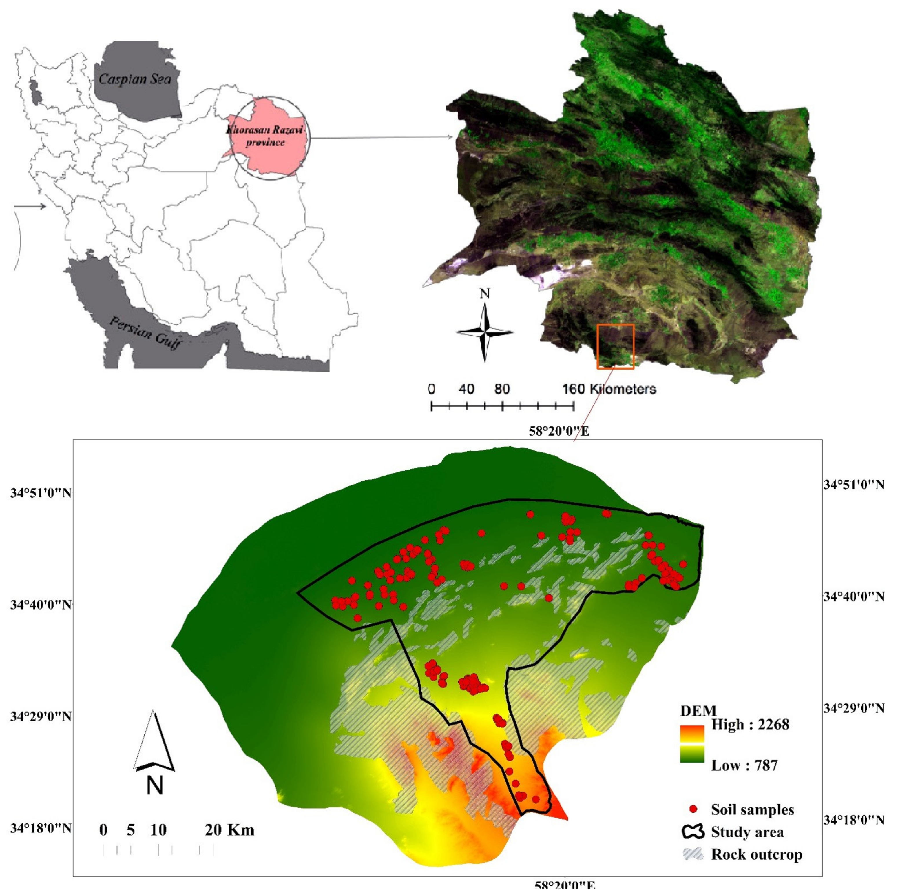
The selected area for study was in Bajestan, a county in Khorasan Razavi province which is located in northeastern Iran. Bajestan has an area of roughly 172,419 ha defined by a rectangle with the following corner coordinates: 34°17′91″ to 34°33′79″ N and 57°57′56″ to 58°00′40″ E (Figure 1) and an elevation range of 786–2283 meters above sea level (m a.s.l) [28]. Pomegranate (Punica granatum L.), pistachio (Pistacia vera L.), and saffron (Crocus sativus L.) are grown in the study area and a variety of landforms and geology are in different parts of the region [28]. According to soil taxonomy [29], the soils are mostly from the Typic Haplocalcids, Typic Torrifluvents, Typic Haplocalcids, and Typic Torripsamments [30].
2.2. Procedures
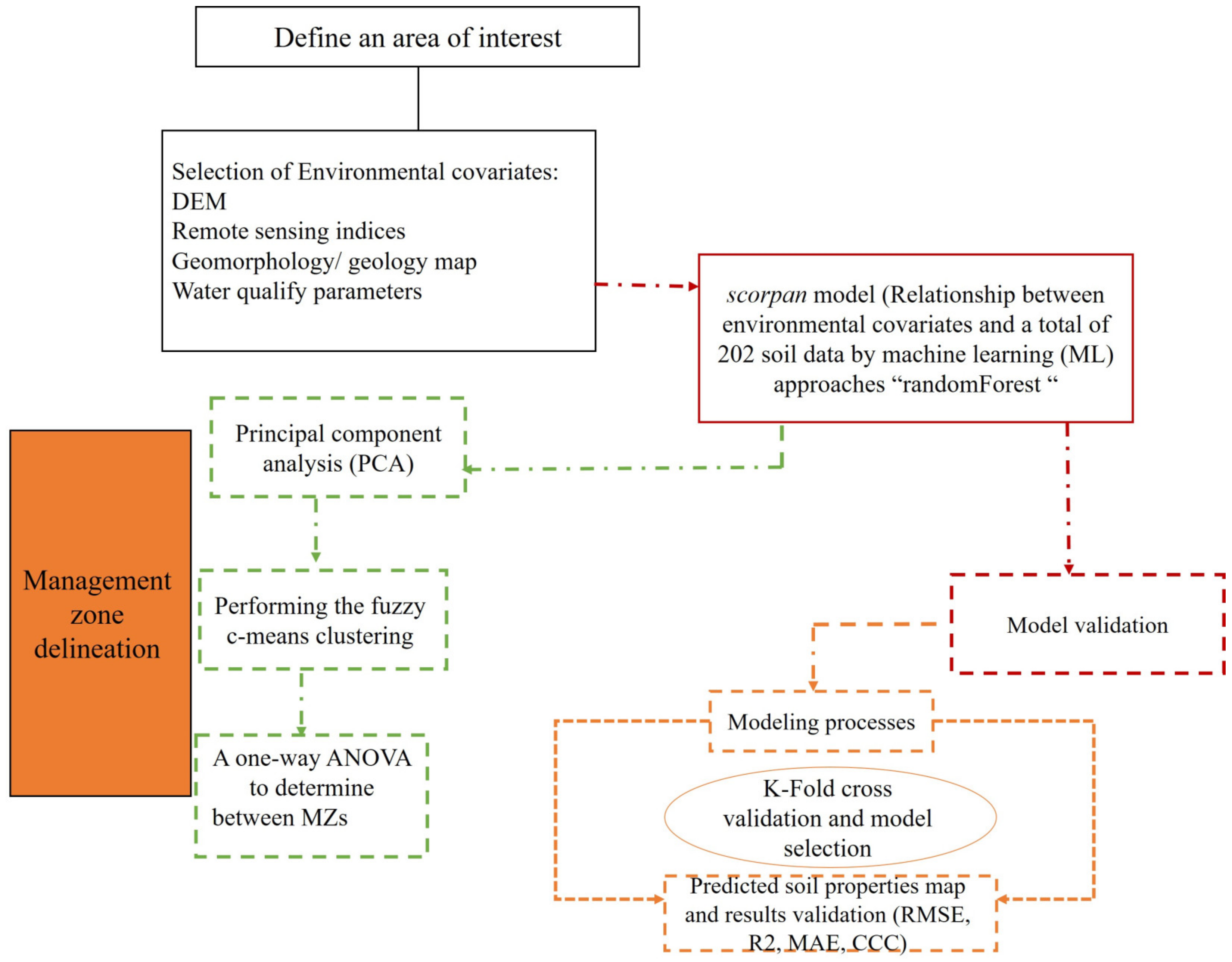
This study completed a series of tasks (Figure 2) including data collection, data analysis and soil property modeling, determination of MZs, statistical analysis, and soil fertility recommendations.
2.3. Soil Field and Laboratory Analysis
The soil samples were taken from a depth of 0–30 cm at 202 locations. All soil samples were air-dried and then sieved. The content of calcium carbonate equivalent (CCE) and soil organic carbon (SOC) were evaluated by titration method [31,32]. Standard laboratory measurement methods were used to measure soil acidity (pH) [33], electrical conductivity (EC) [34], soil texture fractions [35], total nitrogen (TN) [36], available phosphate (Pav) [37], available potassium (Kav) [38], soluble calcium (Ca++), magnesium (Mg++), and sodium (Na+) [39]. The equation in [40] was used to calculate the amount of sodium adsorption ratio (SAR).
2.4. Spatial Variability of Soil Properties
In the current research, the DSM approach [41,42,43,44,45] was used to predict soil properties by analyzing the relationships between environmental covariates and soil properties [45,46,47,48,49]. The environmental covariates used to infer different soil property distributions were tabulated in Table S1. Twenty-one terrain attributes were extracted from a shuttle radar topography mission (SRTM) 1 arc-second DEM (http://earthexplorer.usgs.gov, accessed on 15 July 2020) with spatial resolution 30 m. SAGA-GIS version 2.2 was utilized to calculate terrain derivative attributes [50]. RS indices were extracted from Sentinel 2 (https://sentinel.esa.int/web/sentinel/missions, accessed on 15 July 2020) imagery [51]. In order to prepare a map of water quality parameters, a total of 190 groundwater features, including qanat and wells, were sampled and analyzed according to standard procedures [52]. Then, spatial analyst of ArcMap GIS was used to generate different useful maps for better understanding the variability of water quality in the study area. Groundwater quality parameters (HCO3−, Cl−, SO42−, Na+, Ca++, Mg++, EC, pH, SAR, and TDS) were mapped using geostatistical analysis using the inverse distance weighting (IDW) method [28].
2.5. Random Forests (RF)
Random forests (RF) are decision-tree based models [41,53] which consist of growing sets of trees in the decision tree model [53]. The “ntree” and “mtry” are important parameters that are determined according to number of trees and effective environmental covariates, respectively, in each random subset. The number of environmental covariates can range from one to the total number of independent variables. The number of trees is selected by the user and usually varies from 500 to 1000 [41,53]. It is possible to select the most important effective factors by determining variable importance. The environmental factors with relative importance scores of less than 15% are considered unimportant and are removed from the model [54]. Basically, RF models compute the most important environmental factors by the mean decrease in impurity. The caret package of R3.3.1 was used to predict soil properties for mapping with the RF function [55].
To assess the RF model, a k-fold cross-validation approach was employed. The data were divided into k folds, with one fold serving as the validation set and the remaining k-1 folds used for training. This process was repeated K times, and the average performance was utilized as a metric to evaluate the model. Furthermore, four common indices, including the coefficient of determination (R2), Lin’s concordance correlation coefficient (CCC), mean absolute error (MAE), and root mean square error (RMSE), were used to validate the performance of the RF model. Higher R2 and CCC values and lower MAE and RMSE values show a better model performance based on these validation criteria [56,57].
2.6. Delineation of Management Zones (MZs)
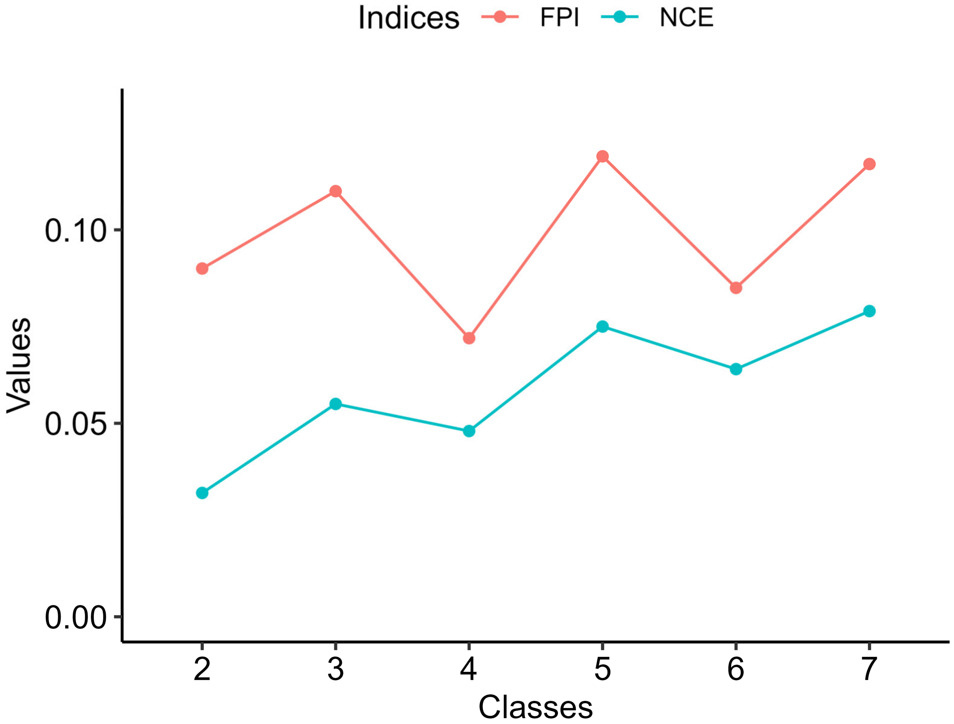
To develop MZ classes, principal component analysis (PCA) was first applied to group the variables into principal components in IBM SPSS 22 statistics software. PCs with eigenvalues ≥ 1.0 were selected throughout the study area. PCs calculate the maximum variance in a data set by linearly combining the variables and describing the vectors. The fuzzy k-means algorithm was then employed to delineate the study area into different exclusive management areas with the aim of producing homogeneous MZs and statistically minimizing intra-group variability and at the same time maximizing inter-group variability [58]. The MZ analyst software (version 1.0, University of Missouri, Columbia, MO, USA) and the fuzzy k-means clustering FuzME software [59] were used as an unsupervised continuous classification procedure to generate homogeneous MZs [16,60] for dividing farmland into 2 to 7 clusters. This clustering algorithm uses PCs obtained from PCA as input for the cluster analysis. This algorithm creates a continuous grouping of objects with the aim of grouping soil and environmental covariates and assigning partial class membership. A random set of cluster averages results in the membership of each cluster as an iterative process. According to the observation distance to the cluster average, the new averages were re-calculated for each cluster. The settings used in the FuzME software for the study area were as follows: maximum number of repetitions = 300, stop criterion = 0.0001, minimum number of zones = 2, maximum number of zones = 7 and the fuzziness exponent = 1.5 [16,60], respectively. The fuzzy performance index (FPI) and the normalized classification entropy (NCE) were calculated to show the degree of fuzziness and the amount of disorganization to determine the best number of clusters [61]. FPI is the degree of fuzziness created by a specified number of classes and its values may range from 0 to 1. Generally, values close to zero indicate distinct classes with little membership sharing and values close to one indicate distinct classes with a high degree of membership sharing. In addition, the NCE is estimated as the amount of disturbance caused by a certain number of classes. Overall, the lowest membership share (FPI) and the highest amount of organization (NCE) create the best number of clusters [16].
Using IBM SPSS 22 statistics software, descriptive statistics of the studied properties and a one-way analysis of variance were performed using the least significant difference (LSD) test to determine significant heterogeneous changes (p ≤ 0.05) between MZs [62]. Spatial analysis and mapping of the studied properties was performed in Arc GIS 10.3 software.
3. Results and Discussion
3.1. Descriptive Statistics for Soil Properties
The mean of EC was >4 dS m−1, indicating that salinity is a major challenge in the area. EC ranged from 0.14 to 46.46 dS m−1. In fact, EC values ranged from non-saline to extremely saline (Table 1). This supports past results that indicate there is excessive soil salinity in central Iran [63,64]. The high standard deviation (SD) (6.30 dS m−1) and coefficient of variation (CV) of 84% emphasize the vast variability of EC in the current study. CVs were categorized as low (<15%), medium (15–35%), high (35–75%), and extremely high (75–150%) variation [65]. The lowest and highest CVs related to pH and Pav, respectively, while the other properties were either high or very high, and sand had moderate CVs (Table 1).
Sand, Silt, and CCE showed moderate variability (12 ≤ CV < 60%) (Table 1). The high CVs (CV ≥ 60%), for EC, clay, SOC, TN, Pav, Ca++, Mg++, Na+ and SAR indicate high variability of nutrients. Additionally, the results of several studies and according to our findings, soil phosphorus had the highest variability [9,24,66] which can be caused by using different phosphorus fertilizers and different management approaches by farmers in areas with diverse cultivation patterns. There was positive skewness (>2) and kurtosis (>3) for EC values which indicates a non-normal distribution of salinity. The SAR ranged from 0.46 to 41 with a mean of 11.57 which shows that the soils range from extremely sodic to non-sodic levels and had high SD and CV values.
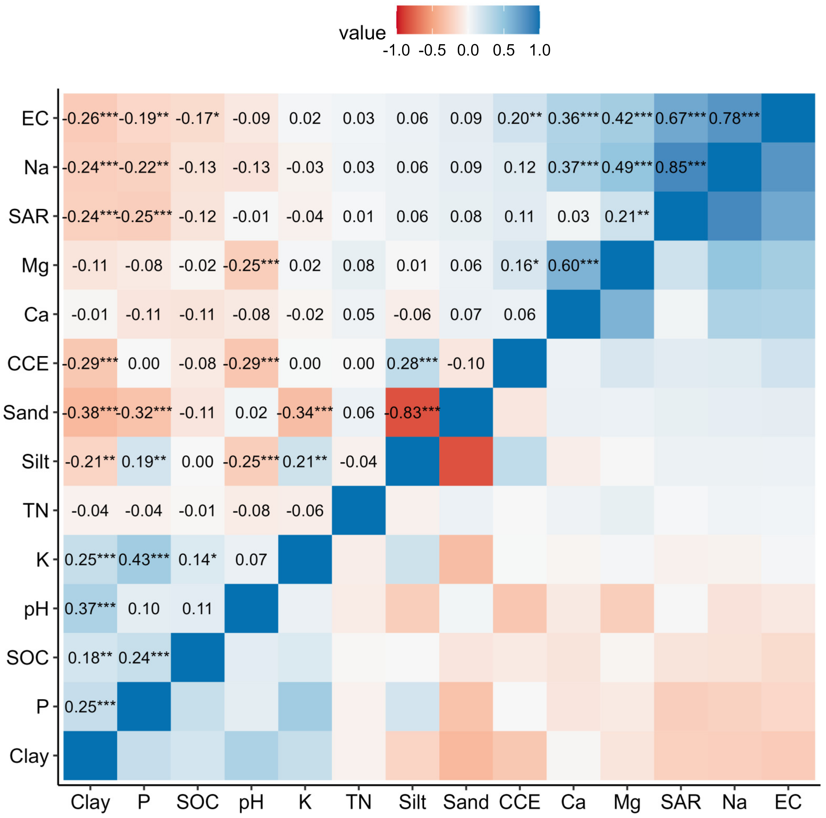
The most significant positive correlations were observed between six variables: TN and SOC (r = 0.89), SAR and Na+ (r = 0.85), Na+ and EC (r = 0.78), SAR and EC (r = 0.66), Mg++ and Ca++ (r = 0.60), and Pav and SOC (r = 0.56). Na+ and EC (r = 0.78), SAR and EC (r = 0.66), and SAR and Na+ (r = 0.85) illustrated positive correlations (Figure 3). The highest significant negative correlation was observed between silt and sand (r = −0.82) (Figure 3) but this is not a true correlation as silt and sand are part of a composition. Other negative correlations were all weak.
3.2. Random Forest Prediction Accuracy
The validation results of soil property maps showed the highest R2 = 0.69 for TN (Table 2). In addition, the validation of map predictions of different soil properties indicated R2 > 0.50 and CCCs = 0.65–0.79 in the study area. Taghizadeh-Mehrjardi et al. [63], Mulder et al. [67], Gomes et al. [68] and Reddy et al. [57] all reported that an R2 ≤ 0.5 is more common and >0.7 is less common in prediction of soil properties. Therefore, the RF model mapped soil spatial variability well in this study. Additionally, RMSE and MAE results for all soil properties except for Kav (RMSE = 67.58 and MAE = 46.0) and Na+ (RMSE = 28.57 and MAE = 18.71) were excellent. There was a very small positive bias for predicted values for all parameters (Table 2) which RMSE and MAE exhibited a positive value with regard to the overestimated prediction of the DSM of soil property. This bias seemed closely related to the average distance of soil sampling, differences of type of cultivated lands and laboratory methods.
The high ranges of Na+ (Min = 0.46 meq L−1, Max = 272.0 meq L−1) and Kav (Min = 17.0 mg kg−1, Max = 695.0 mg kg−1) may be the result of different management by farmers in using chemical fertilizer and irrigation water of different qualities. High variations in the distribution of soil particle size influence the capability to retain soluble salts in the soil, and these variations are connected to geological conditions [28]. It may also be that, due to the extent of the study region and limited soil data, using more soil samples in the validation data would improve the R2. These results are consistent with other studies that showed good performance by RFs for predicting soil properties with reasonable RMSE and bias [64,69,70,71]. In this study, the sampling distance was large; therefore, as Jiang et al. [60], de Oliveira et al. [72] and Zeraatpisheh et al. [10] reported, denser sampling may be needed in future studies for more effective soil property mapping.
3.3. Spatial Prediction of Soil Properties
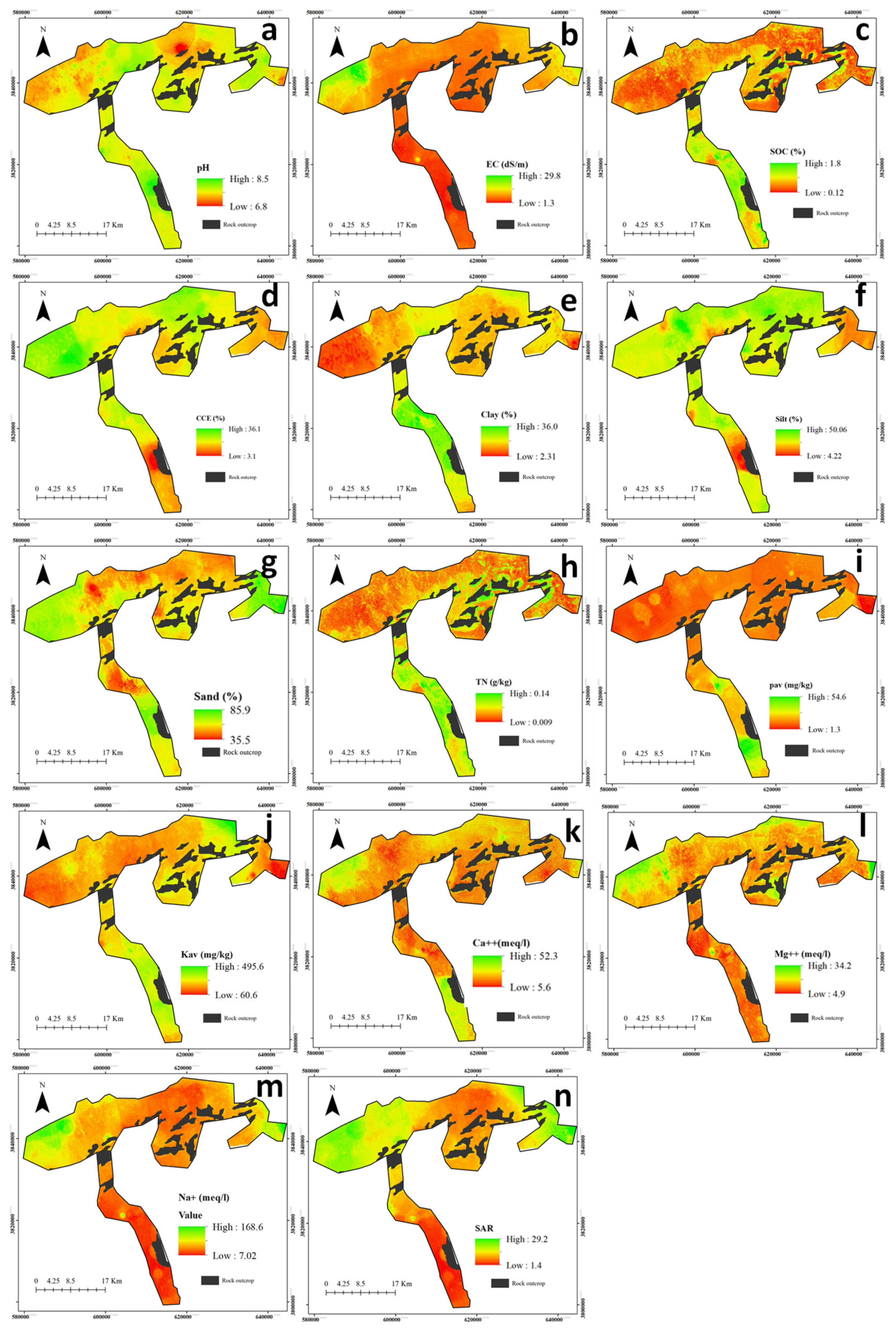
The prediction maps of the studied soil properties showed that the north-western part of the study area had the lowest soil pH value (Figure 4a). Low amounts of EC were found in the soils through the center and south of the study area (Figure 4b). The predicted SOC map (Figure 4c) showed that the highest amount is present in the southern parts and in most of the region, especially in the central, north-eastern, and north-western parts of the area, minimal levels of organic carbon were observed. The reason for naturally low amounts of SOC is the arid climate of this region. However, management of the soils by farmers with the use of animal manure or organic fertilizers have caused changes in the amount of SOC in some areas of the study region (CV = 98.21%). The highest and lowest amounts of CCE were found in the north and north-western part and western parts, respectively, which is related to the geology of area (Figure 4d).
Differences in the soil particle size distribution are varied in the region (Figure 4) due to the sediments and soils of this region being affected by different stratigraphic deposits and elevations. The spatial pattern of TN, as shown in Figure 4h, showed a similar pattern to SOC, as exhibited in Figure 4c (r = 0.89, p < 0.01). The Pav and Kav exhibited a low value from the northwest to the northeast and a high value to the south, with a nearly homogeneous spatial pattern over the rest of the study region. Based on the maps of TN, Pav and Kav, higher values of these three properties were observed in the southern regions (Figure 4i,j). These areas have better conditions for the growth and cultivation of more products such as pomegranate and the highest amount of SOC, which provides the ability to grow a greater variety of crops. Zeraatpisheh et al. [9] expressed the advantages of the prediction map of properties related to soil fertility, including TN, Pav and Kav to make fertilizer recommendations and showed that areas with the highest amounts of these three properties have better conditions for growing and producing more citrus fruits in the north of Iran and Mazandaran province.
The maps shown in Figure 4, illustrate that the distribution of Ca++ was very similar to the Mg++ distribution except in the southern regions, which had higher values of Ca++. It seems that low levels of Ca++ and Mg++ in the central part of the region frequently occurred where there were low amounts of clay. In addition, due to the relationship between Na+ and SAR (r = 0.85, p < 0.01), as well as the initial composition of salt, groundwater with alkaline conditions, and the use of alkaline fertilizers in the region, the spatial change maps of Na+ and SAR represented a similar distribution in the southern part of the region (Figure 4m,n).
The SAR and EC were high and very high in the northern portion of the region where pistachio is grown (Figure 4). Groundwater quality maps (based on SAR, Na+, TDS, Cl−, EC, Ca++, and Mg++) reveal that the associated groundwater parameters are also high in the same area [28]. Cultivated lands of the north are in close proximity of Bajestan playa (Kavir-e Namak), which is another important factor that contributes to high salinity and SAR in this area. This is particularly true in the northwestern part of the region. This is the location of the saltiest part of the playa. Maleki et al. [28] and Taghizadeh-Mehrjardi et al. [63] reported similar findings in studies of the variation of soil properties in the Bajestan region and soil salinity prediction in the Ardakan region of Yazd Province. In some sections of the northern part of the region, heavy soil texture (clay) also increases salt retention. Improper water management on irrigated cultivated lands in northern Bajestan that have low slopes and poor natural drainage has enhanced the salinity of groundwater, changed the depth of the water table, and salinized the soils above it. Raiesi [73] and Nabiollahi et al. [71] highlighted the role of increasing soil salinity in decreasing SQ in arid and semiarid regions. Groundwater and gradual salinization of soil have been observed in the study area. Bhutta and Alam [74] showed that saline soils increased by approximately 17 million ha (from 56% to 73%) between 1953–1954 and 2001–2003 due to the dropping water table and increased salinity from over-pumping of groundwater.
3.4. Principal Component Analysis (PCA)
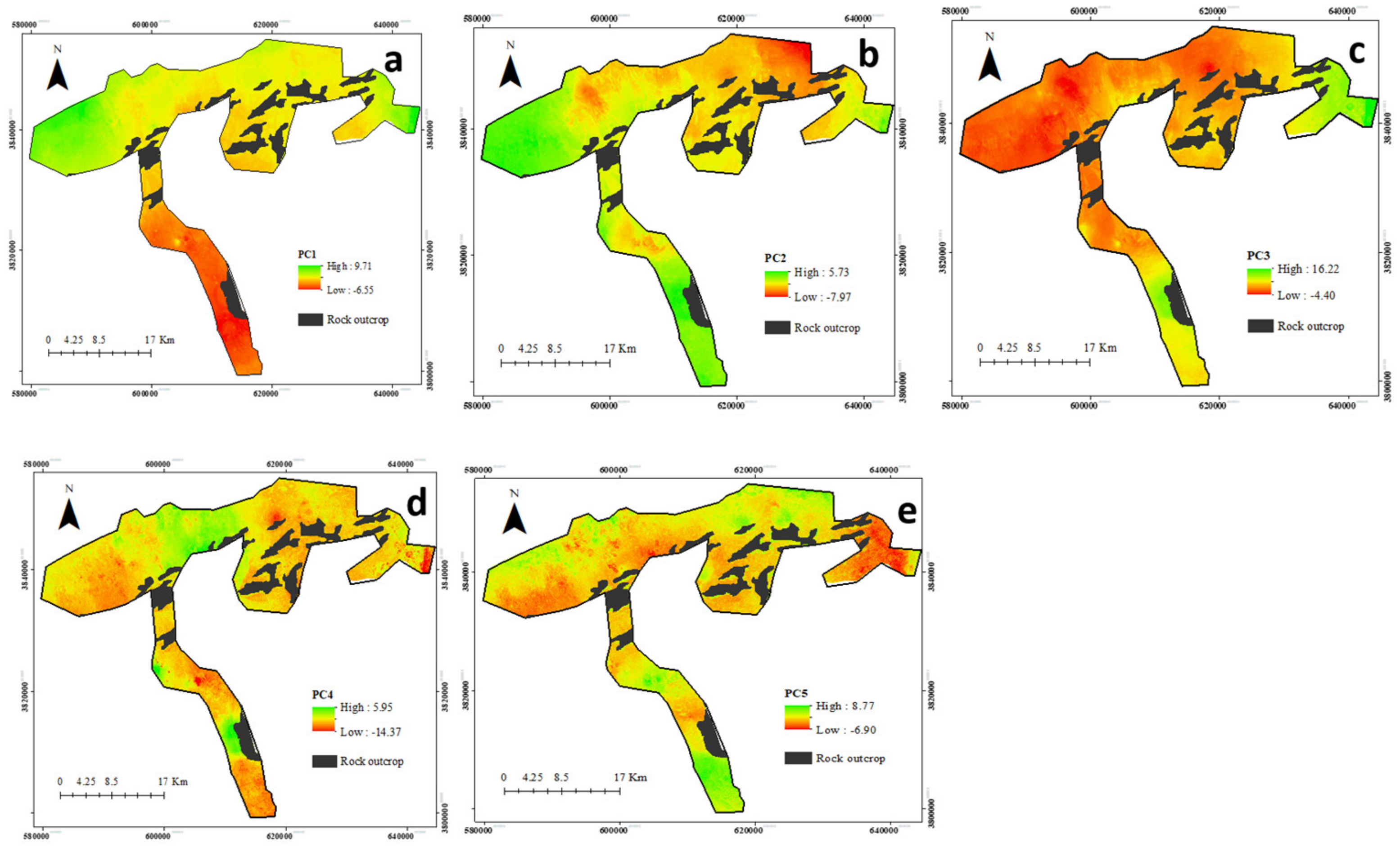
As shown in Table 3, PCA is a good method for summarizing parameter effects because of the high correlation between some soil properties. PCs with eigenvalues >1.0 represented 73.76% of the dataset variability in the study area (Table 3). PC1 accounted for most of the total data variance (25.68%), with the strongest positive loading factors for EC, Na+, and SAR. The map of PC1 showed the high values in north and northeastern parts of the study area (Figure 5a) similar to SAR, Na+, and EC distribution (Figure 4). PC2 explained 17.27% of the total variance and had the strongest loadings for sand (large negative loading factor) and silt (large positive loading factor). The higher values of PC2 (Figure 5b) coincide with the sand map (Figure 4). PC3 had the strongest loadings for SOC, TN, Pav, and Kav and had positive loading factors that explained another 12.43% of the total variance of the dataset. PC3 has high values in part of the southern area (Figure 5c) where TN and SOC maps showed the higher values. PC4 explained 9.40% of the data variation with strong positive loading factors for pH and clay and negative loading factors for CCE (Table 3) and the distribution map of PC4 (Figure 5d) showed similar changes to the mentioned soil properties maps (Figure 4). The last PC (PC5) described 8.96% of the data variability with a positive loading factor for Ca++ and Mg++ (Table 3 and Figure 5e). Thus, five principal components (PC1, PC2, PC3, PC4, and PC5) were used to delineate the MZs for the study region. Davatgar et al. [19] used PCA and “fuzzy k-means” to distinguish MZs for a paddy field in the north of Iran and reported that 72.95% of soil property changes were described by three PCs. Zeraatpisheh et al. [9], in a study in Iran, used PCA and fuzzy c-means to define soil MZs in citrus orchards and stated that four PCs could explain 78.66% of the variation in soil properties. Accordingly, the PCA method incorporated 14 input variables into five new PCs which explain most of the spatial variation of these properties.
3.5. Clustering Analysis
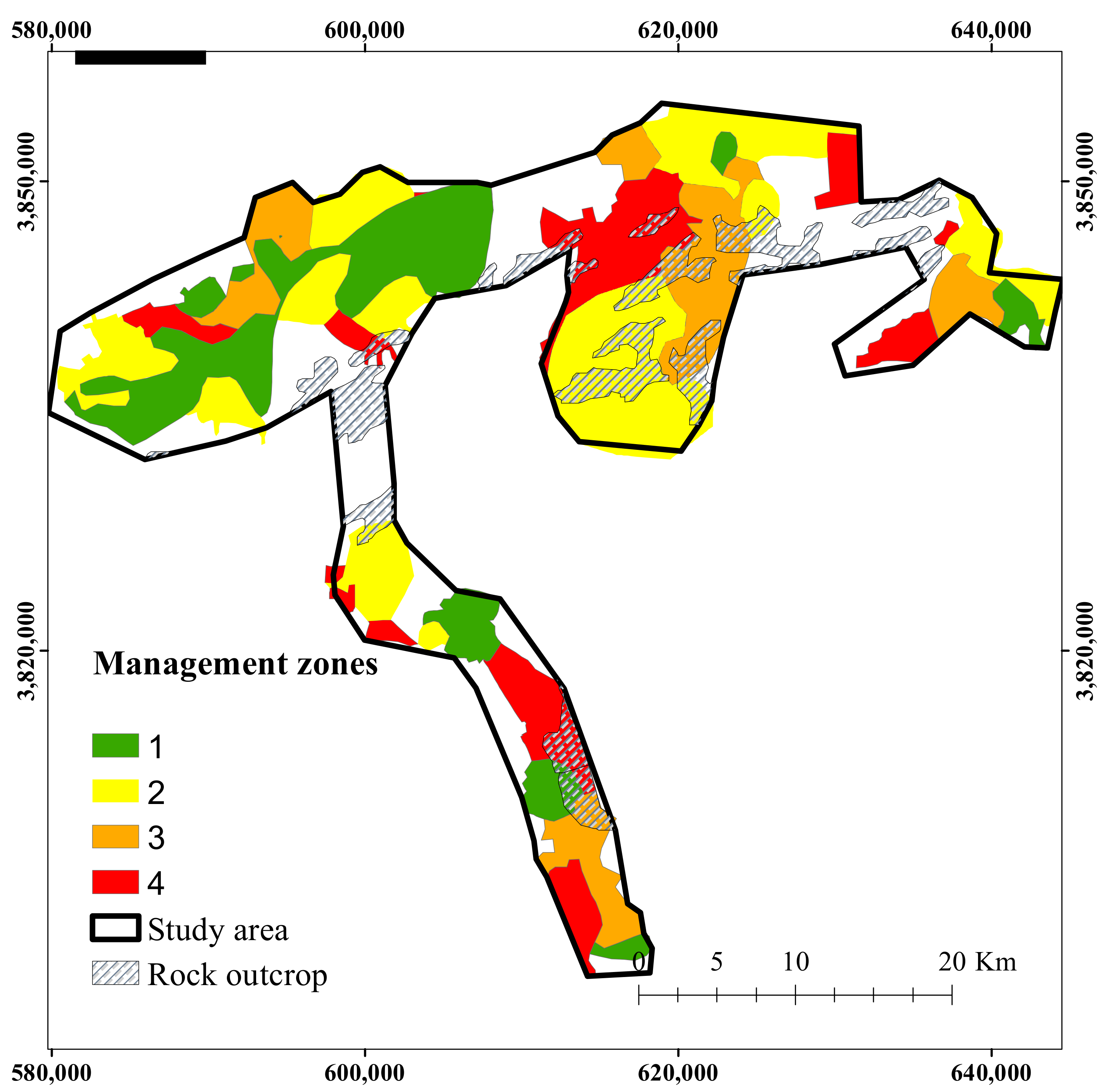
Five PCs were used with cluster analysis to define MZs. The FuzMe software was used to run the “fuzzy k-means” clustering on the five PCs. This method allows differentiation between different areas with similar properties. Hence, when the FPI and NCE values were negligible, the optimal number of MZs could be distinguished, as shown in Figure 6. Four MZs were chosen as optimal as this is where the FPI is at a minimum and NCE is at its second-lowest value. A one-way analysis of variance (ANOVA) was performed to assess the effectiveness of the combination of the PCA clustering algorithm and “fuzzy k-means” to delineate MZs as well as their spatial variability. The four different MZs that were distinguished as the optimal are shown in Figure 7. Several studies reported good results using the analysis of variance to delineate areas [18,61,75]. Zeraatpisheh et al. [9] performed a recent study where two MZs were detected by the fuzzy k-means method in an area in Darab city, Iran.
Based on the results obtained from Table 4, there were significant differences (p < 0.05) between some soil properties except for sand, SOC, TN, Pav, and Ca++ for the four MZs. In comparison to other MZs, pH showed a significant difference in MZ4; clay and Kav showed significant differences in MZ3; and Mg++, Na+, and SAR showed a significant difference in MZ2. MZ3 had lower clay and SOC values and could have lower potential soil fertility than the other zones. This suggests that in this area, more chemical fertilizers and organic fertilizers are needed to increase SOC in MZ3. Generally, the ordering of MZs was MZ4 > MZ1 > MZ3 > MZ2 in relation to soil fertility for all investigated soil properties, based on the results in Table 4. These results can be useful for deciding how to distribute fertilizer in each zone with an emphasis on regionally specific decision making for agriculture lands to allow more sustainable production and, in turn, to reduce environmental risks from uneven application of chemical fertilizers.
3.6. Management Zones (MZs) and Fertilizer Recommendation
Figure 7 shows the MZ map with four MZs. ANOVA was used to evaluate differences in soil nutrients among MZs. There was a significant difference (p < 0.05) between the MZs for each of the soil properties (Table 4). Soils in MZ4 with higher values of clay and SOC and lower values of EC and SAR showed higher soil fertility potential than other zones. There was greater variability in EC and SAR between MZs (Table 4). Mean EC values in MZ2 and MZ3 were 10.45 and 7.78 dS m−1, respectively. Similar to EC, the highest values of SAR were found under MZ2 and MZ3 with values greater than 10. The greatest TN, Pav, and Kav deficiencies occurred in MZ2. The most common reason for these deficiencies in this unit could be the result of reduced capacity of mineral fertilizers and insufficient clay content in this zone. It appears that native N input (low OC) and higher N reduction by leaching (low clay content) limited MZs.
MZ3 contained Pav and Kav around 12.23 and 291.90 mg kg−1 with these areas appearing to have sufficient soil nutrients. MZ4 has the best intrinsic soil fertility due to higher clay, SOC, and nutrient reserves. However, the area of this zone was 16,211.32 ha and MZ2 had the highest area at about 24,580.50 ha (Figure 7).
Maleki et al. [43] predicted SQ maps in earlier study using two datasets (total data set–TDS and minimum data set–MDS) by linear (L) and nonlinear (NL) scoring methods from 223 surface soil samples (0–30 cm depth). The results of the soil quality indices (SQIs) map indicated the maximum values of the SQIs in the southern and central parts of the study area, while the minimum values were found in the north of the study area due to higher EC and SAR. The DSM-predicted soil property maps generated here were transformed to SQI maps according to Maleki et al. [43] and were classified into five classes of SQ including very high (I), high (II), moderate (III), low (IV), and very low (V). The area of MZs within each SQ grade is presented in Table 5. The findings indicate that there are different SQ grades within each of the four delineated zones.
MZ4 had an area of 16211.32 ha, the largest area, categorized as moderate (III) SQ; although part of the area was in the high class (II) SQ (area of 828.21 ha), while the lowest area of very low (V) SQ was located in MZ4 (Table 5). In contrast, MZ1 contained five SQ grades (Table 5) with 0.47 ha located in very high (I) SQ and 66.16 in very low (V).
The results for SQ maps [43] showed that the lower grades of SQ with the highest EC and SAR levels were in the northern portion of the study area in proximity to the playa where elevations are the lowest and topographic wetness index (TWI) is highest [76]. Soil salinity and alkalinity are subject to two primary and secondary factors in the study area. The primary agent includes the conditions of the physical environment (climate, geology, and topography). The secondary factor includes the human uses of the land and management practices (particularly the use of poor-quality irrigation water and inadequate agricultural operation that increase the likelihood of salinity, alkalinity, and sodicity).
The results of Table 6 show the main restricted indicators in each MZ regarding SQI. According to the results of SQ and MZs (Table 6), prescription of fertilizer should be applied based on the uniform fertilization management within each SQ or MZ area. It should be noted that determining the amount of fertilizer required in each region is based on available and common fertilizers used by farmers in the region. Reducing production costs, increasing the quantity and quality of the product, and keeping the environment and soil safe from pollution are potential advantages of fertilizing based on specialized prescriptions and in line with sustainable agricultural practices. Numerous researchers have also reported the distribution of different fertilizers based on MZ delineation [9,10,11,18,19,72].
The fertilization method is very important in the nutritional management of plants. Fertilization should be performed in such a way that the elements required by the plant are provided to the plant in a suitable form and at the desired time. Various factors, such as the type of fertilizer and plant species, affect the fertilization method. In addition, the amount and time for the applied fertilizers will be different in different regions. To increase the efficiency of fertilizers, the management approach and method of consumption have been taken into consideration. The amount of phosphorus in the region is relatively low to medium; in general, it indicates the relative poverty of this element in the soils of the region. However, the deficiency is not as severe as nitrogen (TN < 0.05). Therefore, nitrogen fertilizer consumption should be given serious attention. In order to achieve the highest absorption efficiency of chemical fertilizers for phosphorus, it should be used at the right time and according to the needs of the plant.
The results in Table 4 show that the amount of potassium is relatively moderate amount with a significant difference in terms of this element in MZ3 (Table 6) and other cases (probably due to the difference in soil texture and cultivation pattern). Potassium plays an important role in plant resistance to disease. Among its other important roles, it is possible to regulate the work of stomata openings and water relations and accelerates the growth of generative tissues. Most importantly, the special conditions of the region, which is under the stress of drought, wind, and sometimes cold, should be considered. Therefore, it is necessary to use potassium in the form of potassium sulfate fertilizer in the soils of the region.
The findings showed that farmlands in the study area are generally lacking in SOC (<0.70%), especially in MZ2 and MZ3 with the low amount <0.40 (Table 4 and Table 6). The lack of SOC is one of the most notable problems of the study region. Considering the importance of soil organic matter, increasing it as the first priority for improving soil fertility in plant nutrition management should be given serious attention (Table 6).
Annual applications of gypsum or liquid organic sulfur and organic fertilizers in appropriate ratios to promote effective leaching of salt may be a highly effective approach to remediation of saline and sodic soils. Determining the appropriate cultivation pattern based on MZ maps and changing cultivation towards greenhouse crops can lead to sustainable agriculture and prevent soil degradation. Recognition of the importance of irrigation, water quality, and the patterns of SQ predictions on the MZs map provides scientific guidance for enhanced management of the soils of the Bajestan area, for developing more sustainable agricultural practices. This approach can also be applied in similar regions through DSM.
4. Conclusions
It is necessary to check the fertility status of the soil over time to prevent the depletion of elements from the soil and to replace them at appropriate levels. However, monitoring the soil fertility status should be performed using a low-cost technique and input data so that farmers know which areas have similar production potential. The optimal number of MZs was determined to be four by PCA and the “fuzzy k-means” method. A one-way ANOVA demonstrated significant differences between different MZs in terms of the measured soil properties. The soil fertility indices measured in this case study demonstrated that the low amount of SOC, TN, Pav, and Kav appear to be the main restriction of sustainable production, due to the lower TN, Pav, and Kav of the soil. Application of mineral fertilizers N, P, and K is therefore needed. N, P, and K management are crucial to keep the crop yield at a high level. Moreover, these results showed that by reducing the variability within the zone, the development of MZs through cluster analysis will allow farmers to use more site-specific management. Average soil nutrient values can be used as a guide to calculate the ratio of fertilizer distribution in different areas. Nevertheless, incorporating yield values into this system could improve the rate and timing of fertilizer applications. Generally, as an inexpensive approach to predicting soil properties over large areas and subsequently determining MZs is suggested as a way to improve the accuracy of maps and decrease soil sampling.
Every farmer is faced with different cost strategies and different performance levels for fertilizer use. Based on the available capital, the farmer considers a cost of buying different fertilizers in order to reach a certain performance goal, which creates a different amount of nutrients for the soil. The results of this study will help the farmer to choose the optimal fertilizer combination. Therefore, the optimal amount of fertilizer should be determined considering the soil analysis tests.
Supplementary Materials
Author Contributions
Conceptualization, S.M. and A.K.; methodology, S.M.; R.T.-M. and A.K.; software, S.M., A.M. and R.T.-M.; validation, S.M. and R.T.-M.; formal analysis, S.M., A.K. and R.T.-M.; investigation, S.M. and A.K.; resources, S.M. and A.K.; data curation, S.M.; writing—original draft preparation, S.M., A.K., A.M. and R.K.; writing—review and editing, S.M., A.K., A.M., R.T.-M. and R.K.; visualization S.M. and R.T.-M.; supervision, S.M., A.K. and R.T.-M. Project administration, S.M.; funding acquisition, S.M. All authors have read and agreed to the published version of the manuscript.
Funding
Sedigheh Maleki was partially supported by a grant from Ferdowsi University of Mashhad, Iran (NO. FUM- 14002794075).
Data Availability Statement
The dataset used in this project can be available from the corresponding author on reasonable request.
Acknowledgments
The authors are very grateful to Ferdowsi University of Mashhad and Management of Agricultural Jihad in Bejastan for their financial support and help in soil sampling, respectively.
Conflicts of Interest
The authors declare no conflict of interest.
References
- Yao, R.J.; Yang, J.S.; Zhang, T.J.; Gao, P.; Wang, X.P.; Hong, L.Z.; Wang, M.W. Determination of site-specific management zones using soil physico-chemical properties and crop yields in coastal reclaimed farmland. Geoderma 2014, 232, 381–393. [Google Scholar] [CrossRef]
- Peralta, N.R.; Costa, J.L.; Balzarini, M.; Franco, M.C.; Córdoba, M.; Bullock, D. Delineation of management zones to improve nitrogen management of wheat. Comput. Electron. Agric. 2015, 110, 103–113. [Google Scholar] [CrossRef]
- Ferguson, R.B.; Lark, R.M.; Slater, G.P. Approaches to management zone definition for use of nitrification inhibitors. Soil Sci. Soc. Am. J. 2003, 67, 937–947. [Google Scholar] [CrossRef]
- Castrignanò, A.; Buttafuoco, G.; Quarto, R.; Parisi, D.; Rossel, R.V.; Terribile, F.; Langella, G.; Venezia, A. A geostatistical sensor data fusion approach for delineating homogeneous management zones in Precision Agriculture. Catena 2018, 167, 293–304. [Google Scholar] [CrossRef]
- Franzen, D.W.; Hopkins, D.H.; Sweeney, M.D.; Ulmer, M.K.; Halvorson, A.D. Evaluation of soil survey scale for zone development of site specific nitrogen management. Agron J. 2002, 94, 381–389. [Google Scholar]
- Fraisse, C.W.; Sudduth, K.A.; Kitchen, N.R.; Fridgen, J.J. Use of unsupervised clustering algorithms for delineating within-field management zones. In Proceedings of the International Meeting, Toronto, ON, Canada, 18–21 July 1999; American Society of Agricultural Engineers: St. Joseph, MI, USA, 1999. [Google Scholar]
- Vitharana, U.W.A.; Van Meirvenne, M.; Simpson, D.; Cockx, L.; De Baerdemaeker, J. Key soil and topographic properties to delineate potential management classes for precision agriculture in the European loess area. Geoderma 2008, 143, 206–215. [Google Scholar] [CrossRef]
- Kerry, R.; Ingram, B.; Oliver, M. Sampling needs to establish effective management zones for plant nutrients in precision agriculture. In Precision Agriculture, 1st ed.; Wageningen Academic Publishers: Wageningen, The Netherlands, 2021; pp. 177–192. [Google Scholar]
- Zeraatpisheh, M.; Bakhshandeh, E.; Emadi, M.; Li, T.; Xu, M. Integration of PCA and fuzzy clustering for delineation of soil management zones and cost-efficiency analysis in a citrus plantation. Sustainability 2020, 12, 5809. [Google Scholar] [CrossRef]
- Zeraatpisheh, M.; Bottega, E.L.; Bakhshandeh, E.; Owliaie, H.R.; Taghizadeh-Mehrjardi, R.; Kerry, R.; Scholten, T.; Xu, M. Spatial variability of soil quality within management zones: Homogeneity and purity of delineated zones. Catena 2022, 209, 105835. [Google Scholar] [CrossRef]
- Breunig, F.M.; Galvão, L.S.; Dalagnol, R.; Dauve, C.E.; Parraga, A.; Santi, A.L.; Della Flora, D.P.; Chen, S. Delineation of management zones in agricultural fields using cover–crop biomass estimates from PlanetScope data. Int. J. Appl. Earth Obs. Geoinf. 2020, 85, 102004. [Google Scholar] [CrossRef]
- Cambouris, A.N.; Nolin, M.C.; Zebarth, B.J.; Laverdiere, M.R. Soil Management Zones Delineated by Electrical Conductivity to Characterize Spatial and Temporal Variations in Potato Yield and in Soil Properties. Am. J. Potato Res. 2006, 83, 381–395. [Google Scholar] [CrossRef]
- Medeiros, W.N.; de Queiroz, D.M.; Valente, D.S.M.; Pinto, F.D.A.; Melo, C.A.D. The temporal stability of the variability in apparent soil electrical conductivity. Biosci. J. 2016, 32, 150–159. [Google Scholar] [CrossRef] [Green Version]
- De Assis Silva, S.; Oliveirados Santos, R.; Marçalde Queiroz, D.; Soaresde Souza Lima, J.; FragaPajehú, L.; CarvalhoMedauar, C. Apparent soil electrical conductivity in the delineation of management zones for cocoa cultivation. Inf. Process. Agric. 2022, 9, 443–455. [Google Scholar] [CrossRef]
- Khosla, R.; Inman, D.; Westfall, D.G.; Reich, R.M.; Frasier, M.; Mzuku, M. A synthesis of multi-disciplinary research in precision agriculture: Site-specific management zones in the semi-arid western Great Plains of the USA. Precis. Agric. 2008, 9, 85–100. [Google Scholar] [CrossRef]
- Fridgen, J.J.; Kitchen, N.R.; Sudduth, K.A.; Drummond, S.T.; Wiebold, W.J.; Fraisse, C.W. Management zone analyst (MZA) software for subfield management zone delineation. J. Agron. 2004, 96, 100–108. [Google Scholar]
- Gili, A.; Álvarez, C.; Bagnato, R.; Noellemeyer, E. Comparison of three methods for delineating management zones for site-specific crop management. Comput. Electron. Agric. 2017, 139, 213–223. [Google Scholar] [CrossRef]
- Schenatto, K.; De Souza, E.G.; Bazzi, C.L.; Gavioli, A.; Betzek, N.M.; Beneduzzi, H.M. Normalization of data for delineating management zones. Comput. Electron. Agric. 2017, 143, 238–248. [Google Scholar] [CrossRef]
- Davatgar, N.; Neishabouri, M.R.; Sepaskhah, A.R. Delineation of site specific nutrient management zones for a paddy cultivated area based on soil fertility using fuzzy clustering. Geoderma 2012, 173, 111–118. [Google Scholar] [CrossRef]
- Gavioli, A.; de Souza, E.G.; Bazzi, C.L.; Schenatto, K.; Betzek, N.M. Identification of management zones in precision agriculture: An evaluation of alternative cluster analysis methods. Biosyst. Eng. 2019, 181, 86–102. [Google Scholar] [CrossRef]
- Iticha, B.; Takele, C. Digital soil mapping for site-specific management of soils. Geoderma 2019, 351, 85–91. [Google Scholar] [CrossRef]
- Li, Y.; Shi, Z.; Li, F.; Li, H.Y. Delineation of site-specific management zones using fuzzy clustering analysis in a coastal saline land. Comput. Electron. Agric. 2007, 56, 174–186. [Google Scholar] [CrossRef]
- Taylor, J.C.; Wood, G.A.; Earl, R.; Godwin, R.J. Soil factors and their influence on within-field crop variability, part II: Spatial analysis and determination of management zones. Biosyst. Eng. 2003, 84, 441–453. [Google Scholar] [CrossRef]
- Xin-Zhong, W.; Guo-Shun, L.; Hong-Chao, H.; Zhen-Hai, W.; Qing-Hua, L.; Xu-Feng, L.; Wei-Hong, H.; Yan-Tao, L. Determination of management zones for a tobacco field based on soil fertility. Comput. Electron. Agric. 2009, 65, 168–175. [Google Scholar] [CrossRef]
- Tripathi, R.; Nayak, A.K.; Shahid, M.; Lal, B.; Gautam, P.; Raja, R.; Mohanty, S.; Kumar, A.; Panda, B.B.; Sahoo, R.N. Delineation of soil management zones for a rice cultivated area in eastern India using fuzzy clustering. Catena 2015, 133, 128–136. [Google Scholar] [CrossRef]
- Moharana, P.C.; Jena, R.K.; Pradhan, U.K.; Nogiya, M.; Tailor, B.L.; Singh, R.S.; Singh, S.K. Geostatistical and fuzzy clustering approach for delineation of site-specific management zones and yield-limiting factors in irrigated hot arid environment of India. Precis. Agric. 2020, 21, 426–448. [Google Scholar] [CrossRef]
- Santos, R.O.D.; Franco, L.B.; Silva, S.A.; Sodré, G.A.; Menezes, A.A. Spatial variability of soil fertility and its relation with cocoa yield. Rev. Bras. Eng. Agrícola E Ambient. 2017, 21, 88–93. [Google Scholar] [CrossRef]
- Maleki, S.; Karimi, A.R.; Zeraatpisheh, M.; Poozeshi, R.; Feizi, H. Long-term cultivation effects on soil properties variations in different landforms in an arid region of eastern Iran. Catena 2021, 206, 105465. [Google Scholar] [CrossRef]
- Soil Survey Staff. Keys to Soil Taxonomy, 12th ed.; USDA-Natural Resources Conservation Service: Washington, DC, USA, 2014. [Google Scholar]
- Ghasemzadeh Ganjehie, M.; Karimi, A.R.; Zeinadini, A.; Khorassani, R. Relationship of soil properties with yield and morphological parameters of pistachio in geomorphic surfaces of Bajestan playa, Northeastern Iran. J. Agric. Sci. Technol. 2018, 20, 417–432. [Google Scholar]
- Page, A.L.; Miller, R.H.; Keeney, D.R. Methods of Soil Analysis. In Chemical and Microbiological Properties, Part 2, 2nd ed.; No. 9; ASA, SSSA, CSSA: Madison, WI, USA, 1982; pp. 595–623. [Google Scholar]
- Nelson, D.W.; Sommers, L.E. Total carbon, organic carbon, and organic matter. Chemical and Microbiological Properties. In Methods of Soil Analysis, Part 2; American Society of Agronomy Inc. and Soil Science: Madison, WI, USA, 1996; pp. 961–1010. [Google Scholar]
- Thomas, G.W. Soil pH and Soil Acidity. In Methods of Soil Analysis, Part 3. Chemical Methods; No. 5; American Society of Agronomy Inc. and Soil Science: Madison, WI, USA, 1996. [Google Scholar]
- Rhoades, J. Salinity: Electrical conductivity and total dissolved solids. In Methods of Soil Analysis, Part 3 Chemical Methods; American Society of Agronomy Inc. and Soil Science: Madison, WI, USA, 1996; pp. 417–435. [Google Scholar]
- Gee, G.W.; Bauder, J.W. Particle size analysis. In Methods of Soil Analysis, Part 1; Klute, A., Ed.; American Society of Agronomy: Madison, WI, USA, 1986; pp. 383–411. [Google Scholar]
- Bremner, J.; Mulvaney, C. Nitrogen-total. In Methods of Soil Analysis, Chemical and Microbiological Properties, Part 2; American Society of Agronomy-Soil Science Society of America: Madison, WI, USA, 1982; pp. 595–624. [Google Scholar]
- Olsen, S.R.; Sommers, L.E. Phosphorus. In Methods of Soil Analysis, Part 2 Chemical and Microbiological Properties; Page, A.L., Miller, H., Keeney, D.R., Eds.; American Society of Agronomy Inc. & Soil Science Society of America Inc.: Madison, WI, USA, 1982; pp. 403–429. [Google Scholar]
- Knudsen, D.; Peterson, G.A.; Pratt, P.F. Lithium, sodium and potassium. In Methods of Soil Analysis, Part 2 Chemical and Microbiological Properties; Page, A.L., Miller, H., Keeney, D.R., Eds.; American Society of Agronomy Inc. & Soil Science Society of America Inc.: Madison, WI, USA, 1982; pp. 225–246. [Google Scholar]
- Tucker, B.B.; Kurtz, L.T. Calcium and magnesium determinations by EDTA titrations. Soil Sci. Soc. Am. J. 1961, 25, 27–29. [Google Scholar] [CrossRef]
- Vasu, D.; Kumar Singh, S.; Kumar Ray, S.; Duraisami, V.P.; Tiwary, P.; Chandran, P.; Nimkar, A.M.; Anantwar, S.G. Soil quality index (SQI) as a tool to evaluate crop productivity in semiarid Deccan plateau, India. Geoderma 2016, 282, 70–79. [Google Scholar] [CrossRef]
- Lamichhane, S.; Kumar, L.; Wilson, B. Digital soil mapping algorithms and covariates for soil organic carbon mapping and their implications: A review. Geoderma 2019, 352, 395–413. [Google Scholar] [CrossRef]
- Emadi, M.; Taghizadeh-Mehrjardi, R.; Cherati, A.; Danesh, M.; Mosavi, A.; Scholten, T. Predicting and Mapping of Soil Organic Carbon Using Machine Learning Algorithms in Northern Iran. Remote Sens. 2020, 12, 2234. [Google Scholar] [CrossRef]
- Maleki, S.; Zeraatpisheh, M.; Karimi, A.; Sareban, G.; Wang, L. Assessing Variation of Soil Quality in Agroecosystem in an Arid Environment Using Digital Soil Mapping. Agronomy 2022, 12, 578. [Google Scholar] [CrossRef]
- McBratney, A.B.; Mendonc Santos, M.L.; Minasny, B. On digital soil mapping. Geoderma 2003, 117, 3–52. [Google Scholar] [CrossRef]
- Khaledian, Y.; Miller, B.A. Selecting appropriate machine learning methods for digital soil mapping. Appl. Math. Model. 2020, 81, 401–418. [Google Scholar] [CrossRef]
- Taghizadeh-Mehrjardi, R.; Schmidt, K.; Toomanian, N.; Heung, B.; Behrens, T.; Mosavi, A.H.; Band, S.S.; Amirian-Chakan, A.R.; Fathabadi, A.H.; Scholten, T. Improving the spatial prediction of soil salinity in arid regions using wavelet transformation and support vector regression models. Geoderma 2021, 383, 114793. [Google Scholar] [CrossRef]
- Zeraatpisheh, M.; Ayoubi, S.; Sulieman, M.; Rodrigo-Comino, J. Determining the spatial distribution of soil properties using the environmental covariates and multivariate statistical analysis: A case study in semi-arid regions of Iran. J. Arid Land 2019, 11, 551–566. [Google Scholar] [CrossRef]
- Žížala, D.; Minařík, R.; Skála, J.; Beitlerová, H.; Juřicová, A.; Reyes Rojas, J.; Penížek, V.; Zádorová, T. High-resolution agriculture soil property maps from digital soil mapping methods, Czech Republic. Catena 2022, 12, 106024. [Google Scholar] [CrossRef]
- Kariminejad, N.; Pourghasemi, H.R.; Maleki, S.; Hosseinalizadeh, M. Digital soil mapping of exchangeable sodium percentage in loess derived-soils of Iranian Loess plateau. Geocarto Int. 2022, 1–19. [Google Scholar] [CrossRef]
- Olaya, V.F. A Gentle Introduction to Saga GIS; The SAGA User Group e.V: Göttingen, Germany, 2004; p. 208. [Google Scholar]
- Yue, J.; Tian, J.; Tian, Q.; Xu, K.; Xu, N. Development of soil moisture indices from differences in water absorption between shortwave-infrared bands. ISPRS 2019, 154, 216–230. [Google Scholar] [CrossRef]
- APHA. Standard Methods for the Examination of Water and Wastewater, 9th ed.; American Public Health Association: Washington, DC, USA, 1998; p. 541. [Google Scholar]
- Breiman, L.; Cutler, A. Random forests. Mach. Learn. 2001, 45, 5–32. [Google Scholar] [CrossRef]
- Zhi, J.; Zhang, G.; Yang, F.; Yang, R.; Liu, F.; Song, X.; Zhao, Y.; Li, D. Predicting mattic epipedons in the northeastern Qinghai-Tibetan Plateau using Random Forest. Geoderma Reg. 2017, 10, 1–10. [Google Scholar] [CrossRef]
- R Development Core Team. A Language and Environment for Statistical Computing; R Foundation for Statistical Computing: Vienna, Austria, 2015; Available online: http://www.R-project.org (accessed on 15 December 2015).
- Lawrence, I.; Lin, K. A concordance correlation coefficient to evaluate reproducibility. Biometrics 1989, 45, 255–268. [Google Scholar] [CrossRef] [PubMed]
- Reddy, N.N.; Chakraborty, P.; Roy, S.; Singh, K.; Minasny, B.; McBratney, A.B.; Biswas, A.; Das, B.S. Legacy data-based national-scale digital mapping of key soil properties in India. Geoderma 2021, 381, 114684. [Google Scholar] [CrossRef]
- Brown, D.G. Classification and boundary vagueness in mapping presettlement forest types. Int. J. Geogr. Inf. Sci. 1998, 12, 105–129. [Google Scholar] [CrossRef]
- Minasny, B.; McBratney, A.B. FuzMe, Version 3.0; Australian Centre for Precision Agriculture, The University of Sydney: Sydney, Australia, 2006.
- Jiang, H.L.; Liu, G.S.; Liu, S.D.; Li, E.H.; Wang, R.; Yang, Y.F.; Hu, H.C. Delineation of site-specific management zones based on soil properties for a hillside field in central China. Arch. Agron. Soil Sci. 2012, 58, 1075–1090. [Google Scholar] [CrossRef]
- Behera, S.K.; Mathur, R.K.; Shukla, A.K.; Suresh, K.; Prakash, C. Spatial variability of soil properties and delineation of soil management zones of oil palm plantations grown in a hot and humid tropical region of southern India. Catena 2018, 165, 251–259. [Google Scholar] [CrossRef]
- Barca, E.; Bruno, E.; Bruno, D.E.; Passarella, G. GTest: A software tool for graphical assessment of empirical distributions’ Gaussianity. Environ. Monit. Assess. 2016, 188, 138. [Google Scholar] [CrossRef]
- Taghizadeh-Mehrjardi, R.; Minasny, B.; Sarmadian, F.; Malone, B.P. Digital mapping of soil salinity in Ardakan region, central Iran. Geoderma 2014, 213, 15–28. [Google Scholar] [CrossRef]
- Fathizad, H.; Ardakani, M.A.; Sodaiezadeh, H.; Kerry, R.; Taghizadeh-Mehrjardi, R. Investigation of the spatial and temporal variation of soil salinity using random forests in the central desert of Iran. Geoderma 2020, 365, 114233. [Google Scholar] [CrossRef]
- Carter, M.R.; Gregorich, E.G. Soil Sampling and Methods of Analysis, 2nd ed.; CRC Press: Boca Raton, FL, USA, 2007. [Google Scholar]
- Wilding, L.P.; Dress, L.R. Application of geostatistics to spatial studies of soil. In Advances in Agronomy; Trangmar, B.B., Yost, R.S., Uehara, G., Eds.; Elsevier: Amsterdam, The Netherlands, 1983; p. 38. [Google Scholar]
- Mulder, V.L.; Lacoste, M.; Richer-de-Forges, A.C.; Martin, M.P.; Arrouays, D. National versus global modelling the 3D distribution of soil organic carbon in mainland France. Geoderma 2016, 263, 16–34. [Google Scholar] [CrossRef]
- Gomes, L.C.; Faria, R.M.; de Souza, E.; Veloso, G.V.; Schaefer, C.E.G.R.; Filho, E.I.F. Modelling and mapping soil organic carbon stocks in Brazil. Geoderma 2019, 340, 337–350. [Google Scholar] [CrossRef]
- Xie, X.; Wu, T.; Zhu, M.; Jiang, G.; Xu, Y.; Wang, X.; Pu, L. Comparison of random forest and multiple linear regression models for estimation of soil extracellular enzyme activities in agricultural reclaimed coastal saline land. Ecol. Indic. 2021, 120, 106925. [Google Scholar] [CrossRef]
- Makungwe, M.; MumbiChabala, L.; Chishala, B.H.; MurrayLark, R.M. Performance of linear mixed models and random forests for spatial prediction of soil pH. Geoderma 2021, 397, 115079. [Google Scholar] [CrossRef]
- Nabiollahi, K.; Taghizadeh-mehrjardi, R.; Shahabi, A.; Heung, B.; Amirian-Chakan, A.R.; Davari, M.; Scholten, T. Assessing agricultural salt-affected land using digital soil mapping and hybridized random forests. Geoderma 2021, 85, 114858. [Google Scholar] [CrossRef]
- De Oliveira, J.F.; Mayi, S.; Marchão, R.L.; Corazza, E.J.; Hurtado, S.C.; Malaquias, J.V.; Tavares Filho, J.; Brossard, M.; Guimarães, M.D.F. Spatial variability of the physical quality of soil from management zones. Precis. Agric. 2019, 20, 1251–1273. [Google Scholar] [CrossRef]
- Raiesi, F. A minimum data set and soil quality index to quantify the effect of land use conversion on soil quality and degradation in native rangelands of upland arid and semiarid regions. Ecol. Indic. 2017, 75, 307–320. [Google Scholar] [CrossRef]
- Bhutta, M.N.; Alam, M.M. Prospectives and Limits of Groundwater Use in Pakistan. In Proceedings of the IWMI-ITP-NIH International Workshop on “Creating Synergy between Groundwater Research and Management in South and Southeast Asia”, Roorkee, India, 8–9 February 2005. [Google Scholar]
- Oldoni, H.; Terra, V.S.S.; Timm, L.C.; Júnior, C.R.; Monteiro, A.B. Delineation of management zones in a peach orchard using multivariate and geostatistical analyses. Soil Tillage Res. 2019, 191, 1–10. [Google Scholar] [CrossRef]
- Taghizadeh-Mehrjardi, R.; Nabiollahi, K.; Rasoli, L.; Kerry, R.; Scholten, T. Land Suitability Assessment and Agricultural Production Sustainability Using Machine Learning Models. Agronomy 2020, 10, 573. [Google Scholar] [CrossRef]
- Gallant, J.C.; Dowling, T.I. A multi resolution index of valley bottom flatness for mapping depositional areas. Water Resour. Res. 2003, 39, 1347–1360. [Google Scholar] [CrossRef]
- Conrad, O.; Bechtel, B.; Bock, M.; Dietrich, H.; Fischer, E.; Gerlitz, L.; Wehberg, J.; Wichmann, V.; Bohner, J. System for automated geoscientific analyses (SAGA) v. 2.1.4. Geosci. Model Dev. 2015, 8, 1991–2007. [Google Scholar] [CrossRef]
- Moore, I.D.; Gessler, P.; Nielsen, G.; Peterson, G. Soil attribute prediction using terrain analysis. Soil Sci. Soc. Am. J. 1993, 57, 443–452. [Google Scholar] [CrossRef]
- Bohner, J.; Selige, T. Spatial prediction of soil attributes using terrain analysis and climate regionalization. In SAGA—Analyses and Modelling Applications; Bohner, J., McCloy, K.R., Strobl, J., Eds.; G¨ottinger Geographiche Abhandlungen: Göttingen, Germany, 2006; Volume 115, pp. 13–28. Available online: https://www.semanticscholar.org/paper/Spatial-Prediction-of-Soil-Attributes-Using-Terrain-B%C3%B6hner-Selige/5c565928ba7300053348c7b95ced68c431b923b9 (accessed on 17 November 2022).
- Allbed, A.; Kumar, L. Soil salinity mapping and monitoring in arid and semi-arid regions using remote sensing technology: A review. Adv. Remote Sens. 2013, 2, 373–385. [Google Scholar] [CrossRef]
- Khan, N.M.; Rastoskuev, V.V.; Sato, Y.; Shiozawa, S. Assessment of hydrosaline land degradation by using a simple approach of remote sensing indicators. Agricult. Water Manag. 2005, 77, 96–109. [Google Scholar] [CrossRef]
- Douaoui, A.E.K.; Nicolas, H.; Walter, C. Detecting salinity hazards within a semiarid context by means of combining soil and remote-sensing data. Geoderma 2006, 134, 217–230. [Google Scholar] [CrossRef]
- Ray, S.S.; Singh, J.P.; Das, G.; Panigrahy, S. Use of high resolution remote sensing data for generating site-specific soil management plan. Int. Arch. Photogramm. Remote Sens. Spatial Inf. Syst. B. 2004, 35, 127–131. [Google Scholar]
- Arzani, H.; King, G.W. Application of Remote Sensing (Landsat TM Data) for Vegetation Parameters Measurement in Western Division of NSW; International Grassland Congress: Hohhot, China, 2008; ID NO. 1083. [Google Scholar]
- Chen, Y.; Qiu, Y.; Zhang, Z.; Zhang, J.; Chen, C.; Han, J.; Liu, D. Estimating salt content of vegetated soil at different depths with Sentinel-2 data. Peer J. 2020, 8, e10585. [Google Scholar] [CrossRef]
- Huete, A.R.; Didan, K.; Miura, T.; Rodriguez, E.P.; Gao, X.; Ferreira, L.G. Overview of the radiometric and biophysical performance of the MODIS vegetation indices. Remote Sens. Environ. 2002, 83, 195–213. [Google Scholar] [CrossRef]
- Rondeaux, G.; Steven, M.; Baret, F. Optimization of soil adjusted vegetation indices. Remote Sens. Environ. 1996, 50, 95–107. [Google Scholar] [CrossRef]
- Rouse, J.W.; Haas, J.R.H.; Schell, J.A.; Deering, D.W. Monitoring vegetation systems in the Great Plains withers. In Proceedings of the 3rd ERTS Symposium, Washington, DC, USA, 10–14 December 1974. [Google Scholar]
- Jordan, C.F. Derivation of leaf area index from quality of light on the forest floor. Ecology 1969, 50, 663–666. [Google Scholar] [CrossRef]
- Zinck, J.A. Physiography and Soils. Lecture Notes for Soil Students, Soil Science Division, Soil Survey Courses Subject Matter, K6 ITC, Enschede, The Netherlands, 1989. Available online: https://webapps.itc.utwente.nl/librarywww/papers_1989/tech/zinck_phy.pdf (accessed on 17 November 2022).
- Toomanian, N.; Jalalian, A.; Khademi, H.; Karimian Eghbal, M.; Papritz, A. Pedodiversity and pedogenesis in Zayandeh-rud Valley, central Iran. Geomorphology 2006, 81, 376–393. [Google Scholar] [CrossRef]
Figure 1.
Map of the study region in Iran and the soil points within the study region in relation to a digital elevation model (units are meters above sea level).
Figure 1.
Map of the study region in Iran and the soil points within the study region in relation to a digital elevation model (units are meters above sea level).

Figure 2.
Flowchart of stepwise procedure.

Figure 3.
Pearson correlation coefficients among soil properties. *, **, *** Correlations with p > 0.01 are considered insignificant.
Figure 3.
Pearson correlation coefficients among soil properties. *, **, *** Correlations with p > 0.01 are considered insignificant.

Figure 4.
Maps showing the spatial distribution for all studied soil properties in 0–30 cm: (a) pH, (b) electrical conductivity (EC, dS m−1); (c) soil organic carbon (SOC, %); (d) calcium carbonate equivalent (CCE, %); (e) clay (%); (f) silt (%); (g) sand (%); (h) total nitrogen (TN, %); (i) available phosphorus (Pav, mg kg−1); (j) available potassium (Kav, mg kg−1); (k) Ca++: soluble Ca (meq L−1); (l) Mg++: soluble Mg; (m) Na+: soluble Na; (n) SAR: sodium adsorption ratio.

Figure 5.
Maps showing the spatial distribution of the PCs for all studied soil properties in 0–30 cm: (a) PC1; (b) PC2; (c) PC3; (d) PC4; (e) PC5.
Figure 5.
Maps showing the spatial distribution of the PCs for all studied soil properties in 0–30 cm: (a) PC1; (b) PC2; (c) PC3; (d) PC4; (e) PC5.

Figure 6.
Fuzziness performance index (FPI) and normalized classification entropy (NCE) for the different number of cluster classes defined by PCA and fuzzy k-means.
Figure 6.
Fuzziness performance index (FPI) and normalized classification entropy (NCE) for the different number of cluster classes defined by PCA and fuzzy k-means.

Figure 7.
The management zones map in the study area. White areas are non-agricultural lands.


Table 1.
Descriptive statistical parameters of soil properties of the study area (n = 202).
| Soil Properties | Min | Max | Mean | SD | Skew. | Kurt. | CV (%) |
|---|---|---|---|---|---|---|---|
| EC (dS m−1) | 0.14 | 46.60 | 7.50 | 6.30 | 2.19 | 8.57 | 84.00 |
| pH | 6.10 | 9.10 | 7.83 | 0.45 | −0.52 | 2.00 | 5.75 |
| Sand (%) | 22.00 | 99.50 | 59.82 | 14.96 | −0.33 | −0.42 | 25.01 |
| Clay (%) | 0.00 | 52.00 | 13.75 | 8.58 | 0.93 | 2.08 | 62.40 |
| Silt (%) | 0.00 | 61.20 | 26.37 | 14.15 | 0.13 | −0.66 | 53.66 |
| CCE (%) | 2.00 | 45.00 | 17.63 | 7.39 | 0.92 | 2.88 | 41.92 |
| SOC (%) | 0.02 | 2.47 | 0.56 | 0.55 | 1.47 | 1.51 | 98.21 |
| TN (g kg−1) | 0.00 | 0.24 | 0.05 | 0.04 | 1.36 | 1.36 | 80.00 |
| Pav (mg kg−1) | 0.20 | 80.00 | 10.99 | 11.83 | 2.75 | 10.06 | 107.64 |
| Kav (mg kg−1) | 17.00 | 695.00 | 215.51 | 109.67 | 1.18 | 1.95 | 50.89 |
| Ca++ (meq L−1) | 1.50 | 73.60 | 22.19 | 13.61 | 0.81 | 1.07 | 61.33 |
| Mg++ (meq L−1) | 0.60 | 56.00 | 10.54 | 7.95 | 2.59 | 9.84 | 75.43 |
| Na+ (meq L−1) | 0.46 | 272.00 | 43.76 | 44.37 | 1.57 | 3.50 | 101.39 |
| SAR | 0.46 | 41.00 | 11.57 | 9.63 | 0.76 | −0.14 | 83.23 |
Min: Minimum; Max: Maximum; SD: Standard deviation; Skew: Skewness; Kurt: Kurtosis; CV: Coefficient of variation; EC: Electrical conductivity; CCE: Calcium carbonate equivalent; SOC: Soil organic carbon; TN: Total nitrogen; Pav: Available phosphorus; Kav: Available potassium; Ca++: Soluble Ca; Mg++: Soluble Mg; Na+: Soluble Na; SAR: Sodium adsorption ratio.
Table 2.
Validation criteria for soil property predictions using RF models.
| Soil Properties | RMSE | MAE | CCC | R2 |
|---|---|---|---|---|
| EC (dS m−1) | 0.08 | 0.06 | 0.74 | 0.62 |
| pH | 0.30 | 0.19 | 0.67 | 0.56 |
| Sand (%) | 9.00 | 6.32 | 0.75 | 0.64 |
| Clay (%) | 5.40 | 3.52 | 0.72 | 0.61 |
| Silt (%) | 8.60 | 6.17 | 0.75 | 0.63 |
| CCE (%) | 4.41 | 2.51 | 0.76 | 0.65 |
| SOC (%) | 0.31 | 0.21 | 0.78 | 0.67 |
| TN (g kg−1) | 0.02 | 0.01 | 0.79 | 0.69 |
| Pav (mg kg−1) | 6.66 | 4.02 | 0.78 | 0.66 |
| Kav (mg kg−1) | 67.58 | 46.00 | 0.73 | 0.61 |
| Ca++ (meq L−1) | 9.01 | 6.21 | 0.66 | 0.57 |
| Mg++ (meq L−1) | 5.35 | 3.47 | 0.65 | 0.56 |
| Na+ (meq L−1) | 28.57 | 18.71 | 0.71 | 0.59 |
| SAR | 6.31 | 4.33 | 0.70 | 0.57 |
RMSE: Root mean squared error; MAE: Mean absolute error; R2: Coefficient of determination; CCC: Lin’s concordance correlation coefficient; EC: Electrical conductivity; CCE: Calcium carbonate equivalent; SOC: Soil organic carbon; TN: Total nitrogen; Pav: Available phosphorus; Kav: Available potassium; Ca++: Soluble Ca; Mg++: Soluble Mg; Na+: Soluble Na; SAR: Sodium adsorption ratio.
Table 3.
Results of principal components analysis (PCA) of soil properties (n = 202).
| PC1 | PC2 | PC3 | PC4 | PC5 | |
|---|---|---|---|---|---|
| Proportion of variance % | 25.68 | 17.27 | 12.43 | 9.40 | 8.96 |
| Cumulative proportion of variance % | 25.68 | 42.95 | 55.39 | 64.79 | 73.76 |
| Eigenvalues | 4.10 | 2.76 | 1.98 | 1.50 | 1.43 |
| EC (dS m−1) | 0.81 | −0.04 | −0.16 | −0.13 | 0.25 |
| pH | 0.06 | −0.14 | 0.07 | 0.69 | −0.20 |
| Sand (%) | 0.05 | −0.94 | −0.10 | 0.00 | 0.03 |
| Clay (%) | −0.16 | 0.29 | 0.31 | 0.69 | 0.09 |
| Silt (%) | 0.04 | 0.82 | −0.08 | −0.42 | −0.09 |
| CCE (%) | 0.12 | 0.04 | −0.01 | −0.72 | −0.01 |
| SOC (%) | −0.18 | 0.06 | 0.87 | 0.21 | −0.02 |
| TN (g kg−1) | −0.22 | 0.05 | 0.84 | 0.14 | 0.03 |
| Pav (mg kg−1) | −0.14 | 0.18 | 0.56 | −0.04 | −0.08 |
| Kav (mg kg−1) | 0.09 | 0.28 | 0.73 | 0.04 | 0.02 |
| Ca++ (meq L−1) | 0.15 | −0.04 | −0.07 | −0.01 | 0.94 |
| Mg++ (meq L−1) | 0.46 | −0.00 | 0.34 | −0.25 | 0.61 |
| Na+ (meq L−1) | 0.90 | −0.00 | −0.14 | −0.07 | 024 |
| SAR | 0.87 | −0.01 | −0.23 | 0.00 | −0.11 |
Values in bold correspond, for each variable, to the factor for which the PC value is the largest. Extraction method: Principal component analysis (PCA); EC: Electrical conductivity; CCE: Calcium carbonate equivalent; SOC: Soil organic carbon; TN: Total nitrogen; Pav: Available phosphorus; Kav: Available potassium; Ca++: Soluble Ca; Mg++: Soluble Mg; Na+: Soluble Na; SAR: Sodium adsorption ratio.
Table 4.
Mean values for each management zone and analysis of variance for all studied soil properties.
Table 4.
Mean values for each management zone and analysis of variance for all studied soil properties.
| Soil Properties | MZ1 | MZ2 | MZ3 | MZ4 |
|---|---|---|---|---|
| n | 90 | 48 | 22 | 42 |
| EC (dS m−1) | 6.51 b | 10.45 a | 7.78 ab | 6.10 b |
| pH | 7.79 b | 7.77 b | 7.71 b | 8.03 a |
| Sand (%) | 59.99 a | 60.15 a | 57.55 a | 60.24 a |
| Clay (%) | 13.34 ab | 14.03 ab | 10.47 b | 16.01 a |
| Silt (%) | 26.60 ab | 25.76 ab | 31.94 a | 23.64 b |
| CCE (%) | 18.36 b | 17.07 bc | 21.73 a | 14.56 c |
| SOC (%) | 0.64 a | 0.43 a | 0.38 a | 0.62 a |
| TN (g kg−1) | 0.05 a | 0.03 a | 0.04 a | 0.05 a |
| Pav (mg kg−1) | 11.53 a | 9.26 a | 12.23 a | 11.14 a |
| Kav (mg kg−1) | 194.86 b | 219.91 b | 291.90 a | 214.73 b |
| Ca++ (meq L−1) | 20.58 a | 25.73 a | 21.85 a | 21.77 a |
| Mg++ (meq L−1) | 9.49 b | 14.51 a | 10.05 b | 8.51 b |
| Na+ (meq L−1) | 35.98 b | 70.43 a | 46.30 b | 28.60 b |
| SAR | 9.96 b | 16.15 a | 11.81 b | 9.64 b |
Means with the same letter are not significantly different at the 0.05 probability level based on the least significant difference test. EC: Electrical conductivity; CCE: Calcium carbonate equivalent; SOC: Soil organic carbon; TN: Total nitrogen; Pav: Available phosphorus; Kav: Available potassium; Ca++: Soluble Ca; Mg++: Soluble Mg; Na+: Soluble Na; SAR: Sodium adsorption ratio.
Table 5.
Area of soil quality (SQ) grade within each management zone.
| Quality Index | SQI Range | MZ1 | MZ2 | MZ3 | MZ4 |
|---|---|---|---|---|---|
| I (very high) | >0.639 | 0.47 (0.003%) | - | 0.08 (0.0006%) | - |
| II (high) | 0.529–0.639 | 1004 (6.38%) | 166 (0.68%) | 440 (3.52%) | 828 (5.10%) |
| III (moderate) | 0.418–0.529 | 5903 (37.48%) | 16475 (67.02%) | 7749 (62.0%) | 10518 (64.88%) |
| IV (low) | 0.307–0.418 | 8780 (55.72%) | 7931 (32.27%) | 4289 (34.33%) | 4863 (30%) |
| V (very low) | <0.307 | 66 (0.41%) | 7.6 (0.03%) | 18 (0.15%) | 1.65 (0.0001) |
Table 6.
The restricted limitation of management zones (MZs) related to the area of soil quality (SQ) and land improvement by comparing the difference between site-specific fertilization and uniform management.
Table 6.
The restricted limitation of management zones (MZs) related to the area of soil quality (SQ) and land improvement by comparing the difference between site-specific fertilization and uniform management.
| MZs | Largest Extent of SQI | Restricted Indicators | Suggested Land Improvement |
|---|---|---|---|
| MZ1 | II and III > 70% | Lack of soil nutrient especially TN and Pav | Use of chemical fertilizers (i.e., urea, 46%; triple superphosphate, 46%) and animal manure, leaving plant residuals on the ground |
| MZ2 | III and IV > 99% | Lack of SOC, soil nutrient especially TN, Pav, Kav, and high salinity and SAR | Use of chemical fertilizers (i.e., urea, 46%; triple superphosphate, 46%; potassium sulfate, 46%), sulfur (with 50% purity), and animal manure, leaving plant residuals on the ground |
| MZ3 | III and IV > 96% | Lack of SOC, soil nutrient especially TN, Pav, Kav, and high salinity and SAR | Use of chemical fertilizers (i.e., urea, 46%; triple superphosphate, 46%; potassium sulfate, 46%), sulfur (with 50% purity), and animal manure, leaving plant residuals on the ground |
| MZ4 | II and III > 75% | Lack of soil nutrient especially TN and Pav | Use of chemical fertilizers (i.e., urea, 46%; triple superphosphate, 46%) and animal manure, leaving plant residuals on the ground |
Disclaimer/Publisher’s Note: The statements, opinions and data contained in all publications are solely those of the individual author(s) and contributor(s) and not of MDPI and/or the editor(s). MDPI and/or the editor(s) disclaim responsibility for any injury to people or property resulting from any ideas, methods, instructions or products referred to in the content. |
© 2023 by the authors. Licensee MDPI, Basel, Switzerland. This article is an open access article distributed under the terms and conditions of the Creative Commons Attribution (CC BY) license (https://creativecommons.org/licenses/by/4.0/).
Share and Cite
MDPI and ACS Style
Maleki, S.; Karimi, A.; Mousavi, A.; Kerry, R.; Taghizadeh-Mehrjardi, R. Delineation of Soil Management Zone Maps at the Regional Scale Using Machine Learning. Agronomy 2023, 13, 445. https://doi.org/10.3390/agronomy13020445
AMA Style
Maleki S, Karimi A, Mousavi A, Kerry R, Taghizadeh-Mehrjardi R. Delineation of Soil Management Zone Maps at the Regional Scale Using Machine Learning. Agronomy. 2023; 13(2):445. https://doi.org/10.3390/agronomy13020445
Chicago/Turabian StyleMaleki, Sedigheh, Alireza Karimi, Amin Mousavi, Ruth Kerry, and Ruhollah Taghizadeh-Mehrjardi. 2023. "Delineation of Soil Management Zone Maps at the Regional Scale Using Machine Learning" Agronomy 13, no. 2: 445. https://doi.org/10.3390/agronomy13020445
Note that from the first issue of 2016, this journal uses article numbers instead of page numbers. See further details here.