Smart-Map: An Open-Source QGIS Plugin for Digital Mapping Using Machine Learning Techniques and Ordinary Kriging

Abstract

Machine Learning (ML) algorithms have been used as an alternative to conventional and geostatistical methods in digital mapping of soil attributes. An advantage of ML algorithms is their flexibility to use various layers of information as covariates. However, ML algorithms come in many variations that can make their application by end users difficult. To fill this gap, a Smart-Map plugin, which complements Geographic Information System QGIS Version 3, was developed using modern artificial intelligence (AI) tools. To generate interpolated maps, Ordinary Kriging (OK) and the Support Vector Machine (SVM) algorithm were implemented. The SVM model can use vector and raster layers available in QGIS as covariates at the time of interpolation. Covariates in the SVM model were selected based on spatial correlation measured by Moran’s Index (I’Moran). To evaluate the performance of the Smart-Map plugin, a case study was conducted with data of soil attributes collected in an area of 75 ha, located in the central region of the state of Goiás, Brazil. Performance comparisons between OK and SVM were performed for sampling grids with 38, 75, and 112 sampled points. R² and RMSE were used to evaluate the performance of the methods. SVM was found superior to OK in the prediction of soil chemical attributes at the three sample densities tested and was therefore recommended for prediction of soil attributes. In this case study, soil attributes with R² values ranging from 0.05 to 0.83 and RMSE ranging from 0.07 to 12.01 were predicted by the methods tested.

1. Introduction

Digital mapping of soil and plant attributes provides information allowing variable-rate (VR) application of agricultural inputs [1]. However, the precision of the VR application depends on precision of the maps that are obtained, typically through interpolation among georeferenced samples. In an economically viable sampling system, a range of interpolation methods can be used, including the geostatistical method of Ordinary Kriging (OK), which is popular in digital soil mapping [2]. However, a disadvantage of OK is the need for large numbers of sampling points for semi-variance modeling [3,4].

Recently, with the large volume of information generated in production fields, Machine Learning (ML) techniques have been used as an alternative to OK for digital mapping of soil attributes [5,6,7,8,9]. ML algorithms attempt to discover and quantify patterns among available data to make predictions. Several models that use ML algorithms for prediction and mapping of soil attributes have been developed [7,10,11], among which are Random Forest, Support Vector Machine (SVM), Cubist, K-Nearest Neighbors, and Artificial Neural Networks [10,12,13]. However, to implement ML models for digital mapping, it is necessary to master open-source programming languages such as Python (Python Software Foundation, Wilmington, DE, USA) and R [14].

For the development of applications using ML, several layers of data must be available, such as environmental and climatic variables, soil and plant sensor data, satellite imagery, yield maps, and digital elevation models. These data can be in matrix or vector format, and in various spatial resolutions, which can make the implementation of the ML interpolation model challenging. As many of these features may have a greater or lesser importance in modeling, it may be necessary to use feature selection and elimination techniques [13,15,16].

A computational tool that facilitates the use of ML techniques in digital mapping without requiring programming knowledge can assist users of geographic information systems (GIS) software. QGIS [17] is open-source software featuring a user-friendly interface and an active community of developers and users. Free computer programs are available for Ordinary Kriging, such as Vesper [18], SGeMS [19], DAGApy [20], and KrigMe [21]. However, none of these are available as a QGIS plugin. Given the potential application of ML and the need to integrate QGIS into a system for digital mapping of soil attributes, this study aimed to develop a plugin called Smart-Map that is integrated with QGIS software for digital mapping using OK and ML as interpolation methods.

2. Materials and Methods

Smart-Map was registered with the National Institute of Industrial Property (INPI, Ministry of Economy, Brazil, BR 51 2021 000002-1). Its latest version can be found on GitHub web site. Available online: https://github.com/gustavowillam/SmartMapPlugin (accessed on 25 May 2022) or installed from the QGIS plugin repository. Available online: https://plugins.qgis.org/plugins/Smart_Map (accessed on 25 May 2022). Python 3.7 was used to develop the software, being compatible with macOS, Linux, and Windows operating systems. The graphical user interface (GUI) was designed using PyQt5 (Riverbank Computer Limited, Dorchester, United Kingdom). The software is a plugin to QGIS version 3.10 or higher.

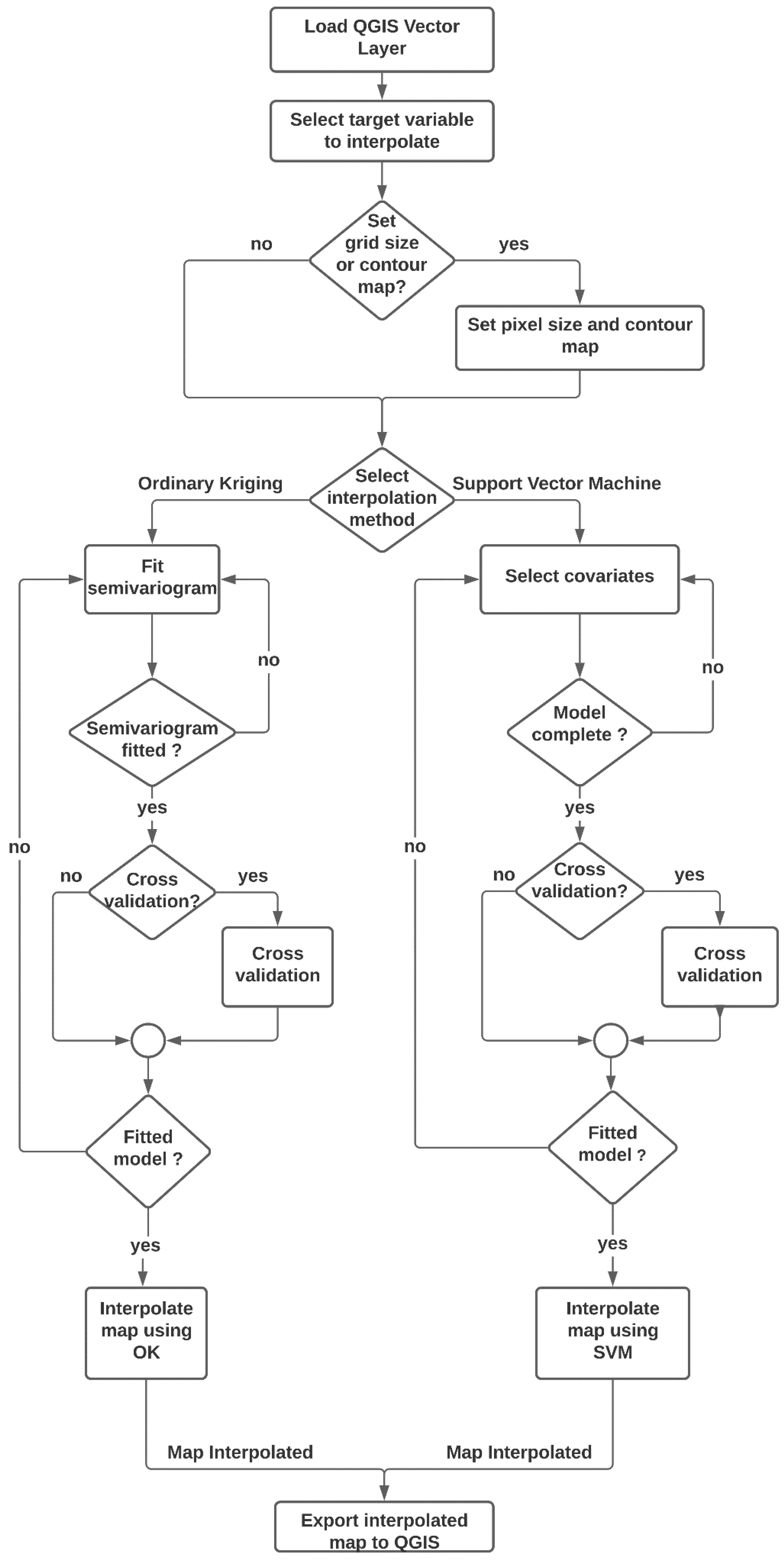
2.1. Smart-Map Implementation

To validate the OK and ML methodology used by Smart-Map, a case study was conducted, where the accuracy of the interpolation of soil attributes was compared using OK and ML for different sampling grids. For the OK interpolation method, the protocols and equations described by [22] were adopted. The developed plugin allows the user to fit five models of isotropic theoretical semivariograms: linear, linear with sill, exponential, spherical, and Gaussian. The semivariogram model was chosen using a cross-validation method.

The Support Vector Machine (SVM) method is a machine learning algorithm, developed in the 1990s and used for both regression and classification of datasets [23]. The SVM method was chosen for interpolation because it can handle smaller and larger volumes of data [24]. For most ML algorithms, it is necessary to fit hyperparameters that need to be chosen by the user because they depend on the data type and variation. For the SVM algorithm, hyperparameters such as C and gamma (γ) were optimized using a systematic grid search method [25,26], enabling automated fitting. Hence, the C and gamma hyperparameters were optimized based on the RMSE value found during cross-validation. Kernel function is another important hyperparameter for SVM. For the plugin, the Radial Basis Function (RBF) kernel was chosen because it is a non-linear function and can be fitted to most of the data.

In addition to the generation of interpolation maps, Smart-Map can perform cluster analyses using the fuzzy k-means method [27], yielding Management Zones (MZ) maps. To define the ideal number of classes, Smart-Map calculates the FPI (Fuzzy Performance Index) and NCE (Normalized Classification Entropy) indices, which are widely recommended in the literature to define the appropriate number of MZs [28,29]. To execute the cluster process and define the MZs, the fuzzy k-means algorithm of the Scikit-Fuzzy Python library was implemented [30]. The flowchart of the Smart-Map plugin is shown in Figure 1, whereas Figure 2 shows the GUI for map interpolation using OK and SVM in Smart-Map.

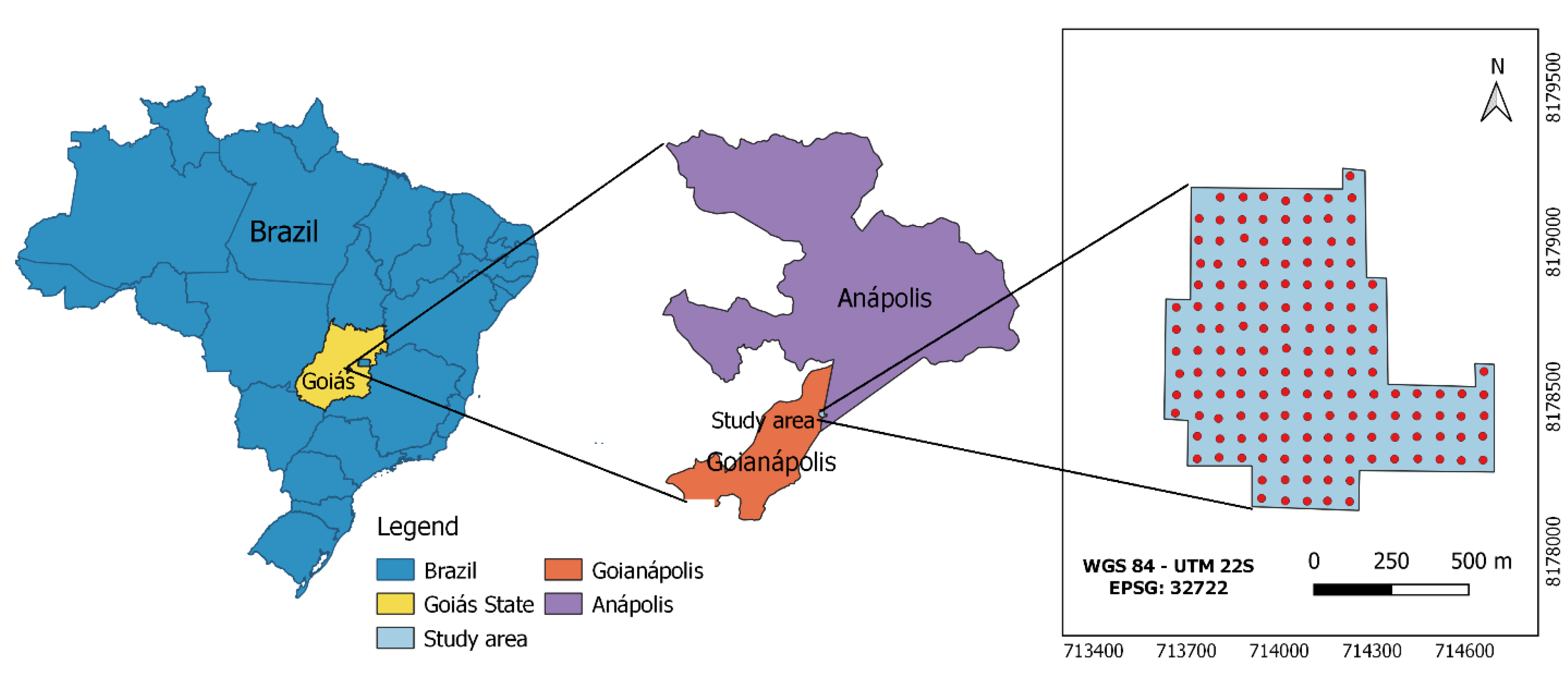
2.2. Case Study for Smart-Map Plugin Evaluation

A case study to evaluate Smart-Map was conducted in an area of 75 ha, located between the municipalities of Anápolis and Goianápolis at latitude and longitude of approximately −16.274839 and −48.593840, in the central region of the state of Goiás, Brazil (Figure 3). This area is cultivated with soybean, has an average altitude of 1017 m, a flat relief with a soil predominantly classified as Ferralsols, based on the World Reference Base for Soil Resources [31]. Soil samples were collected using a regular grid with a sampling density of two points per hectare, totaling 150 composite samples. The samples were georeferenced with a topographic GNSS Promark 3 (Magellan Co., Santa Clara, CA, USA). Each composite sample comprised 10 individual samples (0 to 0.20 m depth), collected within a 3 m radius. Composite samples were homogenized, packed in plastic bags and identified using a composite sample number. Laboratory analyses were performed to measure the concentrations of macronutrients (P, K⁺, Ca²⁺ and Mg²⁺), organic matter, cation exchange capacity at pH 7, and particle size. Data of apparent soil electrical conductivity (ECa) were also collected on five dates (Eca_1 measured on 11/11/2010, Eca_2 measured on 11/23/2010, Eca_3 measured on 12/04/2010, Eca_4 measured on 12/13/2010 and Eca_5 measured on 01/26/2011) using a portable conductivity meter Landviser LandMapper^® ERM 02 (Landviser LLC, League City, TX, USA). This device measures the electrical resistivity of the soil using four equally spaced electrodes [32]. The apparent electrical conductivity of the soil is obtained by 1/resistivity. The data used in the case study, were made available to the research community [33]. Descriptive statistics of the data are presented in

Table 1. Descriptive statistics of soil attributes in the area of study.

Variable	Unit	Min	Max	Mean	SD (17)	Median	CV(%) (18)
P (1)	mg dm−3	1.70	21.60	6.84	3.96	5.85	57.88
K+ (2)	mg dm−3	24.00	108.00	52.63	14.20	51.00	26.98
Ca2+ (3)	cmolc dm−3	1.90	4.20	3.27	0.46	3.30	14.04
Mg2+ (4)	cmolc dm−3	0.60	1.40	0.84	0.14	0.80	16.53
OM (5)	dag kg−1	2.50	4.30	3.06	0.30	3.10	9.85
CEC (6)	cmolc dm−3	4.20	9.90	5.95	0.86	5.90	14.41
Altitude (7)	m	987	1025	1011.2	7.63	1012.1	0.75
Clay (8)	g kg−1	26.00	44.00	33.11	3.37	33.00	10.17
Silt (9)	g kg−1	6.00	20.00	10.60	2.94	10.00	27.78
Sand (10)	g kg−1	45.00	65.00	56.28	4.41	56.50	7.84
Eca_1 (11)	mS m−1	2.49	8.36	4.92	1.01	4.83	20.62
Eca_2 (12)	mS m−1	2.95	10.00	5.95	1.22	5.99	20.56
Eca_3 (13)	mS m−1	1.71	9.11	4.54	1.13	4.51	24.86
Eca_4 (14)	mS m−1	1.84	7.32	3.98	0.88	3.94	22.09
Eca_5 (15)	mS m−1	0.89	5.57	2.65	0.71	2.61	26.67
Eca_Avg (16)	mS m−1	2.17	8.03	4.41	0.84	4.44	19.08

⁽¹⁾ P, Phosphorus; ⁽²⁾ K⁺, Potassium; ⁽³⁾ Ca²⁺, Calcium; ⁽⁴⁾ Mg²⁺, Magnesium; ⁽⁵⁾ OM, Organic Matter; ⁽⁶⁾ CEC, cation exchange capacity at pH 7; ⁽⁷⁾ Altitude; ⁽⁸⁾ Clay; ⁽⁹⁾ Silt; ⁽¹⁰⁾ Sand; ⁽¹¹⁾ Eca_1, Apparent Soil Electrical conductivity measured on 11/11/2010; ⁽¹²⁾ Eca_2, Apparent Soil Electrical conductivity measured on 11/23/2010; ⁽¹³⁾ Eca_3, Apparent Soil Electrical conductivity measured on 12/04/2010; ⁽¹⁴⁾ Eca_4, Apparent Soil Electrical conductivity measured on 12/13/2010; ⁽¹⁵⁾ Eca_5, Apparent Soil Electrical conductivity measured on 01/26/2011; ⁽¹⁶⁾ Eca_Avg, Mean Value of Apparent Soil Electrical conductivity of Eca_1, Eca_2, Eca_3, Eca_4, Eca_5; ⁽¹⁷⁾ SD, Standard Deviation; ⁽¹⁸⁾ CV, Coefficient of Variation.

.

2.3. Methods of Interpolation and Spatial Correlation Analysis

In the case study, an interpolation grid of 10 m × 10 m was defined to perform interpolation by OK and SVM. To interpolate each point of the grid using OK, the search radius was defined equal to the range obtained by the theoretical semivariogram; the maximum number of neighbors was defined as 16. For interpolation by OK, Smart-Map uses the Python open-source PyKrige library [34]. The PyKrige library performs the interpolation using the k-nearest neighbors method. The library was adapted to also accept the search radius. Interpolation was performed using the k-nearest neighbors method or using a neighborhood search radius, selected by the user.

For interpolation by SVM, a supervised learning model, available in the open-source Scikit-Learn Python library, was implemented [35]. For modeling, it is necessary to construct the X matrix and y vector. The X matrix is composed of columns with the features (covariates) and rows, which are the soil samples. In the X matrix, the geographic coordinates x and y of the point to be interpolated were added as features. In addition to geographic coordinates, other features, including the feature of the variable itself, were added in the X matrix. In this case, the feature is created based on the calculation of the Inverse Distance Weighting (IDW) of the nearest neighbors to the point to be interpolated. The y vector was composed of the observed (true) values of each soil attribute to be interpolated. In this case study, the attributes P, K⁺, Ca²⁺, and Mg²⁺ were interpolated variables. Thus, the observed value obtained for the point is part of the y vector and is not used for feature creation, rather merely the IDW of neighbors of the point were considered. In addition, Smart-Map allows the use of data from other layers in the QGIS database (vector or raster) as features.

In the case study, two methods of modeling by SVM were used, which were termed as SVM1 and SVM2. For the SVM1 method, the geographic coordinates (x and y) and the value of the variable itself, which was estimated using the IDW interpolation method, were used as features. In SVM2, those features that were more correlated with the variable to be interpolated were used as covariates, in addition to the geographic coordinates (x and y) and the value of the variable itself, interpolated using IDW. The selection of covariates was made based on the spatial correlation of Moran’s Index (I’Moran), one of the most popular indices for evaluation of spatial correlation [36] of regionalized variables. The univariate I’Moran was used to compare the degree of correlation of the variable itself in different distance spaces (spatial autocorrelation). The univariate I’Moran measures the autocorrelation of the variable to be interpolated. This index was used as an indicator of the spatial dependence of each attribute [37]. A univariate I’Moran value equal to zero means that the variable under study does not show spatial correlation. The closer the value is to 1 or −1, the greater the autocorrelation, that is, the greater the spatial correlation of the variable [6,38]. Univariate I’Moran was calculated according to Equation (1) [39]. The bivariate I’Moran was used to measure the spatial correlation between the available covariates such as CEC, OM, Altitude, Clay, Silt, Sand, and ECa, with the attribute that was interpolated. Its value was calculated according to Equation (2) [40].

$$I=\frac{n}{{{\displaystyle \sum }}_{i=1}^n{{\displaystyle \sum }}_{j=1}^{n}wij}. \frac{{{\displaystyle \sum }}_{i=1}^n{{\displaystyle \sum }}_{j=1}^n{w}_{ij}\left(x_i-\overline{x}\right).\left(x_j-\overline{x}\right)}{{{\displaystyle \sum }}_{i=1}^n{\left(x_i-\overline{x}\right)}^2}$$

(1)

$$I_{x, y}=\frac{{{\displaystyle \sum }}_{i=1}^n \left[\left({{\displaystyle \sum }}_{j=1}^n{w}_{ij}\left(x_j-\overline{x}\right)\right).\left({{\displaystyle \sum }}_{j=1}^n{w}_{ij}\left(y_j-\overline{y}\right)\right)\right]}{\sqrt{{{\displaystyle \sum }}_{i=1}^n{\left(x_i-\overline{x}\right)}^2}.\sqrt{{{\displaystyle \sum }}_{i=1}^n{\left(y_i-\overline{y}\right)}^2}}$$

(2)

where: $n$ is the number of observations in the area under study; $x_i,x_j$ represent the observed values of the soil attributes to be interpolated at the points i, j; $y_i,y_j$ represent the observed values of the selected covariate at the points i, j; $\overline{x}$ is the average of x; $\overline{y}$ is the average of y;$w_{ij}$ are the elements of the matrix of spatial weights with value 0 on the diagonal (w_ii = 0).

The optimal subset of covariates for the SVM2 method was selected considering the bivariate I’Moran. Covariates that showed greater spatial correlation with the variable to be interpolated were added to the SVM2 method. To verify the significance of I’Moran, the pseudo p-value was obtained from 999 permutations between the points of the sampling grid at 1% and 5% probability levels. For the calculation of I’Moran, Smart-map used the PySAL open-source Python library [41].

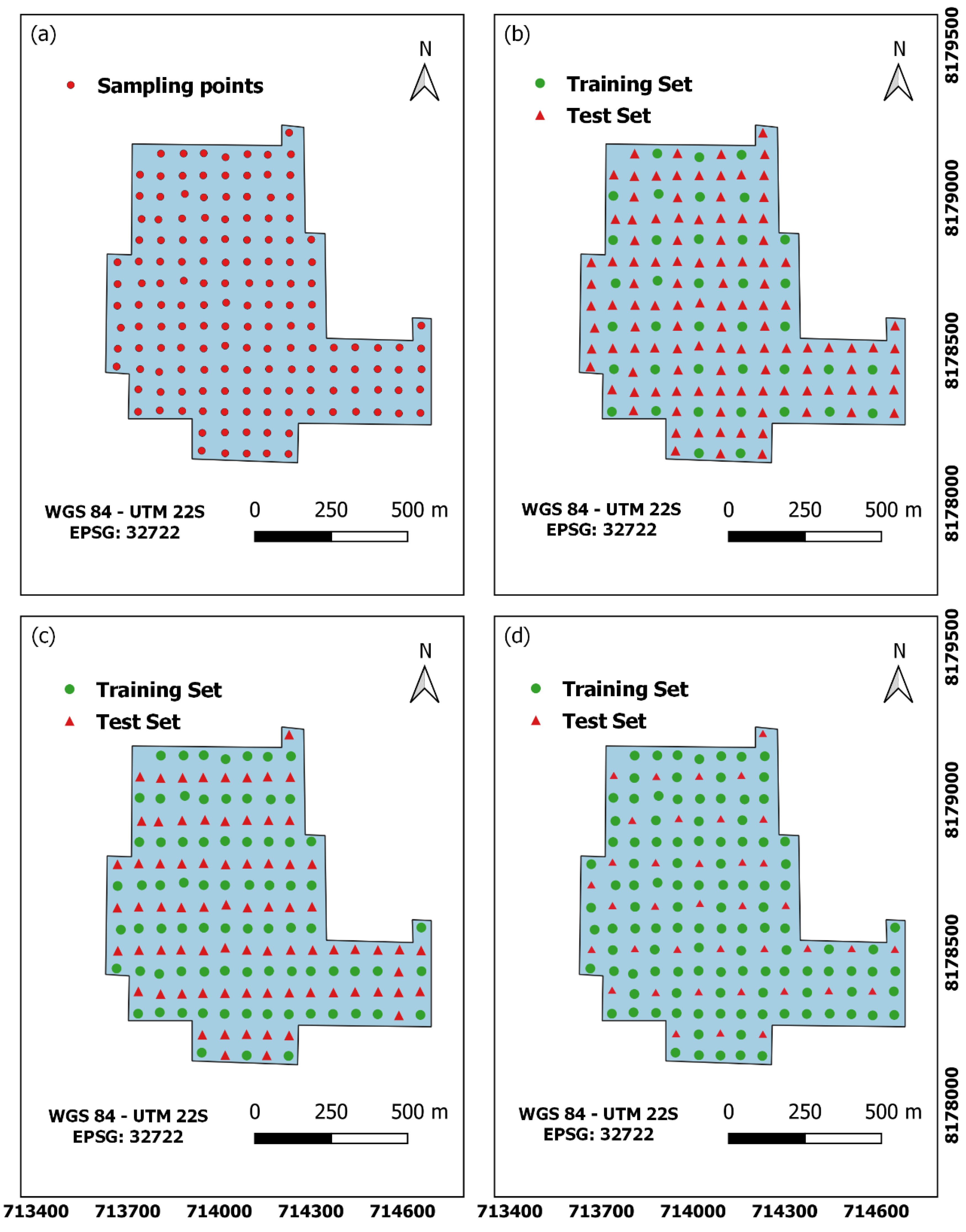
2.4. Generation of Scenarios and Performance Criteria for Comparison between Interpolation Methods

To compare the performance of the OK method and the SVM models (SVM1 and SVM2) at various sampling densities, the regular grid of 150 points in the area was reduced to grids with lower densities (25%, 50%, and 75%). Three grids were obtained with 38, 75, and 112 points, respectively. These points were used for semivariogram modeling in the OK method and definition of the training set in the SVM model, whereas the remaining points were used for verification of the accuracy of the prediction. Figure 4a shows the original grid with 150 points and the reduced grids composed of modeling and testing data. In the grid with 38 points (Figure 4b), 38 points were used for modeling and 112 points for testing. In the grid with 75 points (Figure 4c), 75 points were used for modeling and 75 points were used for testing. In the grid with 112 points (Figure 4d), 112 points were used for modeling and 38 points were used for testing.

From the reduction of the sampling grid, interpolated maps were generated using the sets of training points for the OK method and the SVM model at the three densities of sampling grids. In this case study, the attributes P, K⁺, Ca²⁺, and Mg²⁺ were interpolated. For modeling, the SVM method requires the adjustment of two hyperparameters, C and gamma. K-fold cross-validation was used to obtain optimal values of these hyperparameters. Validation with 5-folds was used to optimize the model in the selection of the best hyperparameters using the training dataset. The leave-one-out cross-validation (LOOCV) [42] method was used to measure the performance of the implemented methods. LOOCV consists of using all data and leaving one data point out and has been widely used due to its mathematical simplicity. The outside point is then interpolated by one of the interpolation methods [43]. This strategy was applied to all samples in the set. As the actual values of the set are known, the Coefficient of Determination (R²) and RMSE values of the LOOCV were calculated. The R² and the RMSE of predicted and observed data of LOOCV were calculated for each model and for each interpolated attribute. The test sets were used to calculate the R² and RMSE of each map obtained by interpolation of P, K⁺, Ca²⁺ and Mg²⁺, after modeling. For this, the interpolated values of P, K⁺, Ca²⁺ and Mg ²⁺ were extracted from the same places where the test points were located. R² and RMSE were calculated using Equations (3) and (4), for P, K⁺, Ca²⁺, and Mg²⁺ for the various sampling grids.

$$R^2=1-\frac{{{\displaystyle \sum }}_{k=1}^n{\left(x_k-\widehat{x_k}\right)}^2 }{{{\displaystyle \sum }}_{k=1}^n{\left(x_k-\overline{x}\right)}^2 }$$

(3)

$$RMSE= \sqrt{\frac{1}{n} {{\displaystyle \sum }}_{k=1}^n{\left(x_k-\widehat{x_k}\right)}^2 }$$

(4)

where:$\widehat{x_k}$ represents the estimated value of the soil attribute at the point k; $\overline{x}$ is the average of the n sampled points of the soil attribute; $x_k$ is the observed value of the soil attribute at the point k; and $n$ is the number of points sampled.

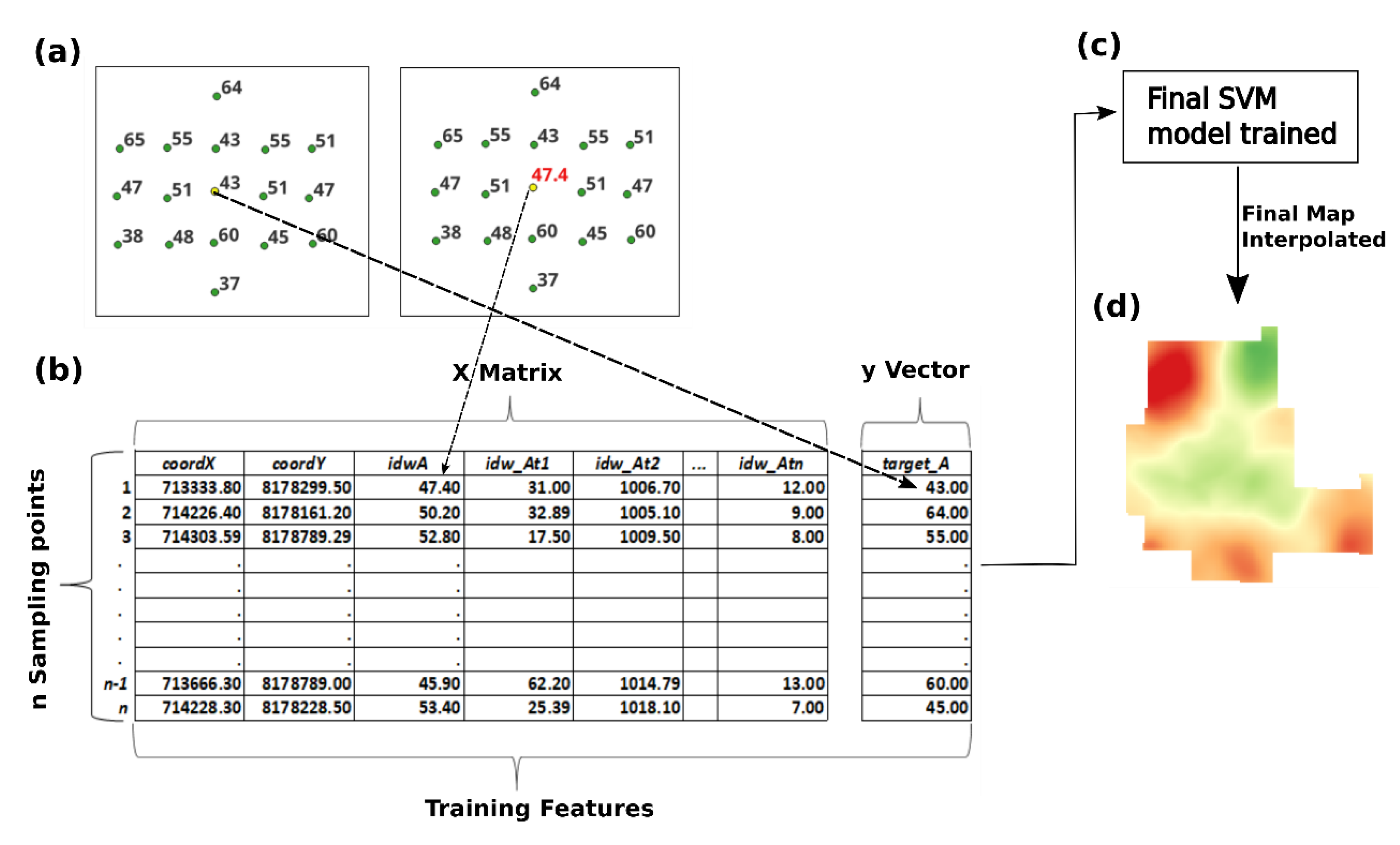
2.5. Definition and Selection of Features for the SVM Model

To define the features to be inserted in the SVM model, the user defines the Inverse Distance Weighting (IDW) parameters such as the weighting value (p), the search radius, and the number of neighbors (n) to consider for calculating the feature for the X matrix. In the case study, a search radius equal to the maximum distance between the sampled points was used, the number of neighbors was equal to 16 and a weight (p) equal to unity were used as default values.

Figure 5a shows a selection of the 16 closest neighbors to the point where the user wishes to estimate the attribute value using the IDW method of the selected attribute of the QGIS layer (target_A). Figure 5b shows how the ML model for the SVM1 and SVM2 methods was constructed divided into features (X matrix) and variable to be interpolated (y vector). Each row of the training data represents a sample of the grid. In the X matrix, coordX and coordY are the x and y coordinates of the sampled point, respectively; idwA represents the estimated value for the variable based on IDW using the 16 neighbors closest to the sampled point of the attribute to be interpolated; idw_At1, idw_At2, idw_Atn represent the estimated value based on IDW using the 16 neighbors closest to the sampled point of the selected features. In the y vector, target_A represents the sampled values of the attribute to be interpolated, which were P, K⁺, Ca²⁺, and Mg²⁺.

For SVM1, the features consisted of the coordinates (coordX and coordY) of the point and the IDW value of the variable (y) using the 16 neighbors closest to the sampled point, within the defined search radius of the attribute to be estimated. The variable to be interpolated (y) represents the observed soil attribute, for which the user wishes to predict its values at unsampled locations. In this case study, the variables are P, K⁺, Ca²⁺ and Mg²⁺.

In the second approach (SVM2), the features were the coordinates (coordX and coordY), and the IDW of 12 covariates available in the study area: OM, CEC, Altitude, Clay, Silt, Sand, ECa_1, ECa_2, ECa_3, ECa_4, ECa_5, and ECa_Avg. In this case, the features used originated from the original grid with 150 points. This was done because the goal of using the SVM is to take advantage of information that has been densely sampled in the area. These data can be obtained by sensors or comprise quasi-static information.

The R² accuracy metric of the LOOCV cross-validation was applied for each subset of covariate added. The subset of covariates that had the best value of R² was chosen to define the SVM model to be used for the variable to be interpolated. This selection was performed considering all features for grids with 38, 75, and 112 sampling points. The final trained SVM model was obtained after performing the LOOCV of all points of the training set (Figure 5c). With the trained model, the interpolation of soil variables (P, K⁺, Ca²⁺, and Mg²⁺) was performed, thus obtaining the interpolated map for the attribute (Figure 5d).

3. Results and Discussion

In this section we discuss the results of the spatial correlation obtained through the I’Moran method between the covariates used by the SVM1 and SVM2 methods and the interpolated variables (P, K⁺, Ca²⁺, and Mg²⁺). In addition, a performance comparison between the OK and SVM methods is discussed. The OK and SVM1 methods used only the estimated value of the variable to be interpolated as an input feature for the model. The SVM2 method used, in addition to the estimated value of the variable, the covariates with the highest spatial correlation with the variable to be interpolated as input for the model.

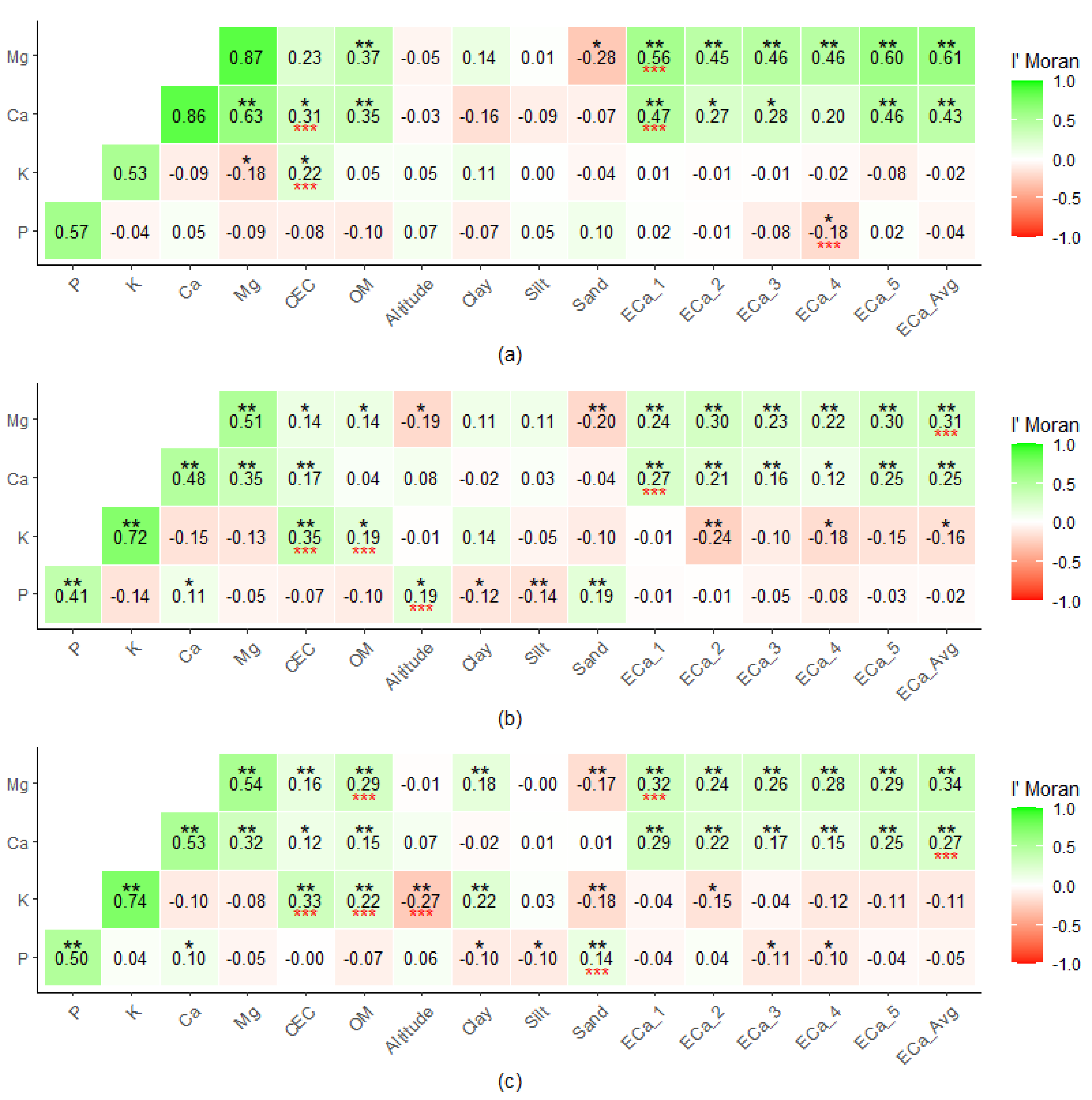
3.1. Spatial Correlation and Selection of Covariates for the SVM Model

For spatial correlation analysis at the three densities of sampling grid, bivariate I’Moran was used to measure the correlation between the contents of the macronutrients P, K⁺, Ca²⁺, and Mg²⁺ and the covariates with highest temporal stability (CEC, OM, Altitude, Clay, Silt, Sand, ECa_1, ECa_2, ECa_3, ECa_4, ECa_5, ECa_Avg). Figure 6 shows the values of univariate I’Moran for the variables to be interpolated (P, K⁺, Ca²⁺, and Mg²⁺) and bivariate I’Moran between the variables to be interpolated and the covariates with greatest temporal stability for the sampling densities of 38, 75, and 112 points.

Figure 6 shows that apparent soil electrical conductivity (ECa) measured on five dates showed a significant positive correlation with the attributes Mg²⁺ and Ca²⁺, with values ranging from 0.12 (between Ca²⁺ and ECa_4, grid of 75 points) to 0.61 (between Mg²⁺ and ECa_Avg, grid of 38 points). For the interpolation of these two soil attributes, ECa was used as a covariate in the SVM2 method at the three densities of sampling grids (Figure 6). In the grid of 38 sampling points (Figure 6a), the covariates ECa_1 for the attributes Mg²⁺ and Ca²⁺ and CEC for Ca²⁺ were used. In the grid with 75 points (Figure 6b), ECa_Avg was used for the Mg²⁺ attribute and ECa_1 was used for the Ca²⁺ attribute. Finally, in the grid with 112 sampling points (Figure 6c), the attributes OM and ECa_1 for Mg²⁺ and ECa_Avg for Ca²⁺ were used as interpolation covariates.

ECa showed low correlations with the attributes P and K⁺, implying a lower potential for use as covariates to interpolate P and K⁺. ECa_4 was used to interpolate only the P attribute in the grid with 38 points, since the correlation was significant with I’Moran of −0.18 (Figure 6a). For the same grid, CEC was used as a covariate for the K⁺ attribute. For the grid with 75 points (Figure 6b), the covariates CEC and OM were used for the K⁺ attribute and the covariate Altitude was used for the P attribute. According to Figure 6b, Altitude presented the highest spatial correction of I’Moran with attribute P, 0.19 and p-value ≤ 0.05, as well as attribute Sand. However, only Altitude was used because presented the best score in LOOCV. For the grid with 112 points (Figure 6c), the K⁺ attribute used the covariates CEC, OM, and Altitude, and the P attribute used Sand as covariate for interpolation.

3.2. Comparison between OK and SVM Methods

For the training set, at three different densities of sampling grids, the values of R² (Figure 7) show that the SVM2 method was superior for the four soil attributes analyzed (P, K⁺, Ca²⁺, and Mg²⁺), except for K⁺ in the grid with 75 points. The univariate I’Moran for the K⁺ attribute was 0.72 and significant at a 1% probability level in the grid with 75 points, as shown in Figure 6b. Values of R² for the SVM2 method in the training set ranged from 0.16 to 0.38. Compared to the SVM1 method, the SMV2 method obtained a higher R² for all attributes analyzed in all point densities of the sampling grids.

OK showed the lowest coefficients of determination values for the attributes P, K⁺, and Ca²⁺ in the grid with 38 points (Figure 7). The values of univariate I’Moran for P and K⁺ were low and not significant for the two soil attributes analyzed (Figure 6a). As mentioned by [2,3], OK requires a minimum number of sampling points for good semivariogram modeling. For the grid with 38 points, the SVM2 method performed better than the OK method, with R² values ranging from 0.19 to 0.38. For the P attribute, the three methods had the lowest values of R². These data corroborate Figure 6, in which the values of univariate and bivariate I’Moran were low for the P attribute. In general, OK, SVM1, and SVM2 showed lower R² values for the grid of 38 sampling points, compared to grids with higher sampling density.

As in the training set, the values of R² were also higher for the SVM2 method in the test set (Figure 8). The lowest correlation coefficient for the SVM2 method was obtained for the P attribute in the sampling grid with 38 points in the test set (R² = 0.15). The low performance of SVM2 for predicting the P attribute is related to the covariate added to the grid with 112 points in the training set. The Sand covariate used by the SVM2 method had bivariate I’Moran of 0.14 with the P attribute (Figure 6c). This value was the lowest used by a covariate added to the SVM2 method. Covariates that have low value of bivariate I’Moran with the attribute to be interpolated may not contribute or contribute in a non-significant way to a better performance of the SVM2 method. [16] claim that the low correlation between predictor variables and the dependent variable (y) directly impacts the performance of the ML model.

The RMSE values for the soil attributes P, K⁺, Ca²⁺, and Mg²⁺, for the OK, SVM1, and SVM2 methods are shown in

Table 2. RMSE values found for P, K⁺, Ca²⁺, and Mg²⁺ for the sampling grids with grid of 38, 75, and 112 sampling points for the training set.

Density	38 Samples			75 Samples			112 Samples
Variable *	OK	SVM1	SVM2	OK	SVM1	SVM2	OK	SVM1	SVM2
P	3.24	2.92	2.85	2.91	3.19	2.80	3.36	3.47	3.32
K+	11.57	10.87	8.94	8.73	9.21	9.03	10.33	10.27	10.09
Ca2+	0.46	0.42	0.40	0.40	0.40	0.38	0.40	0.40	0.39
Mg2+	0.12	0.12	0.11	0.10	0.10	0.10	0.11	0.10	0.10

* P, K⁺ in (mg dm⁻³), and Ca²⁺, Mg²⁺ in (cmolc dm⁻³).

and

Table 3. RMSE values found for P, K⁺, Ca²⁺, and Mg²⁺ for sampling grids with density of 112, 75, and 38 sampling points for the test set.

Density	112 Samples			75 Samples			38 Samples
Variable *	OK	SVM1	SVM2	OK	SVM1	SVM2	OK	SVM1	SVM2
P	3.40	3.36	3.22	3.59	3.04	2.74	2.75	1.94	2.79
K+	9.74	10.05	9.70	12.01	11.77	11.41	9.04	9.46	8.14
Ca2+	0.41	0.29	0.28	0.41	0.26	0.25	0.41	0.24	0.23
Mg2+	0.11	0.11	0.07	0.12	0.10	0.10	0.15	0.14	0.10

* P, K⁺ in (mg dm⁻³), and Ca²⁺, Mg²⁺ in (cmolc dm⁻³).

for the training and test sets, respectively. In Table 2 the training sets with 38, 75, and 112 points were displayed, while in Table 3 their respective test sets are 112, 75, and 38 points, in this order, thus totaling 150 sampled points divided between training and testing. As expected, the RMSE values tended to be lower for greater values of R² for the training set (Figure 7 and Table 2) and for the test set (Figure 8 and Table 3). Similar results have been observed in other studies [5,15]. With lower RMSE values (Table 2), it can be inferred that OK was superior to SVM1 in the prediction of P, as the R² was similar (R² = 0.11 and 0.15 in the grids of 75 and 112 points, respectively) as shown in Figure 7.

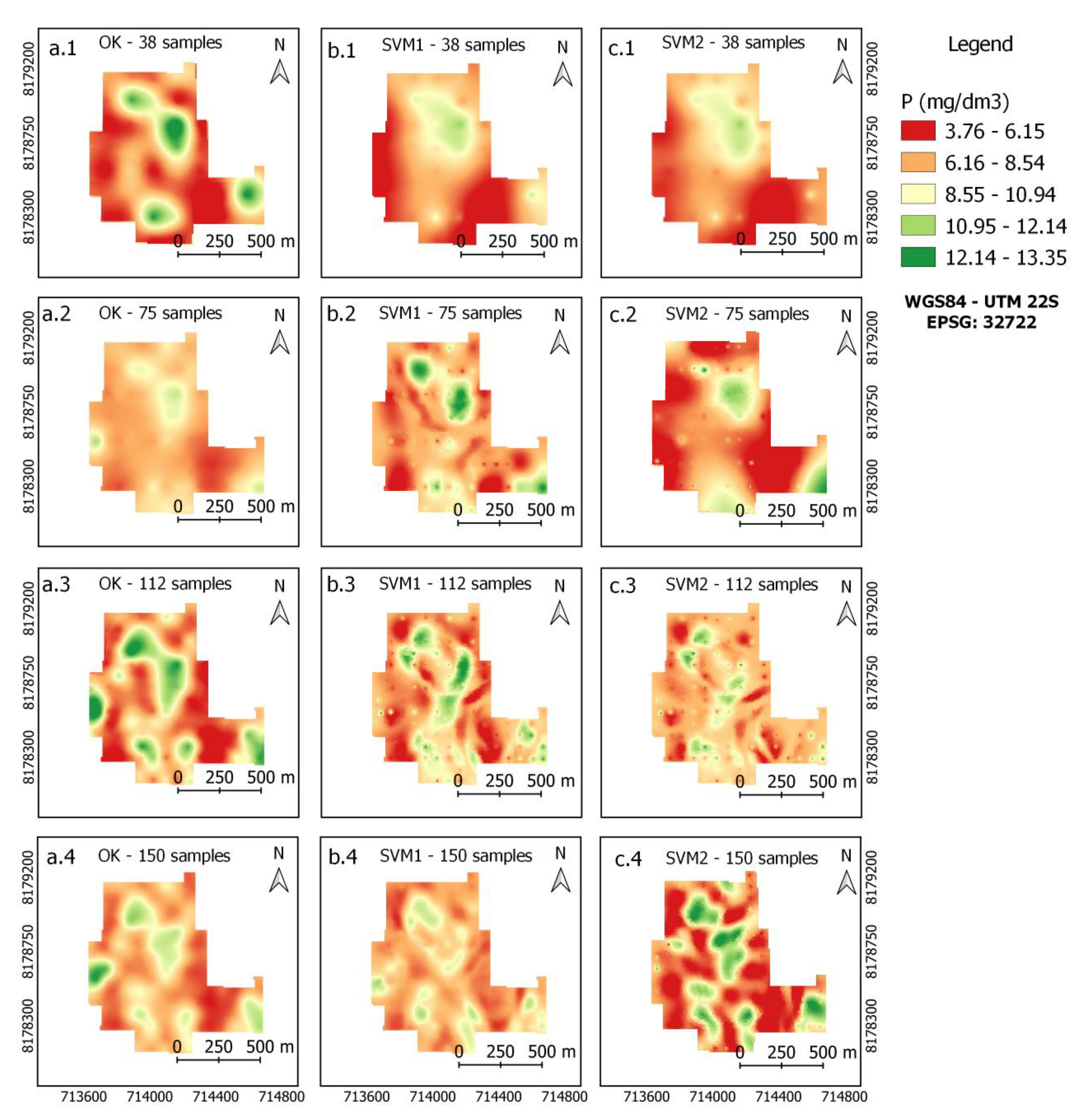
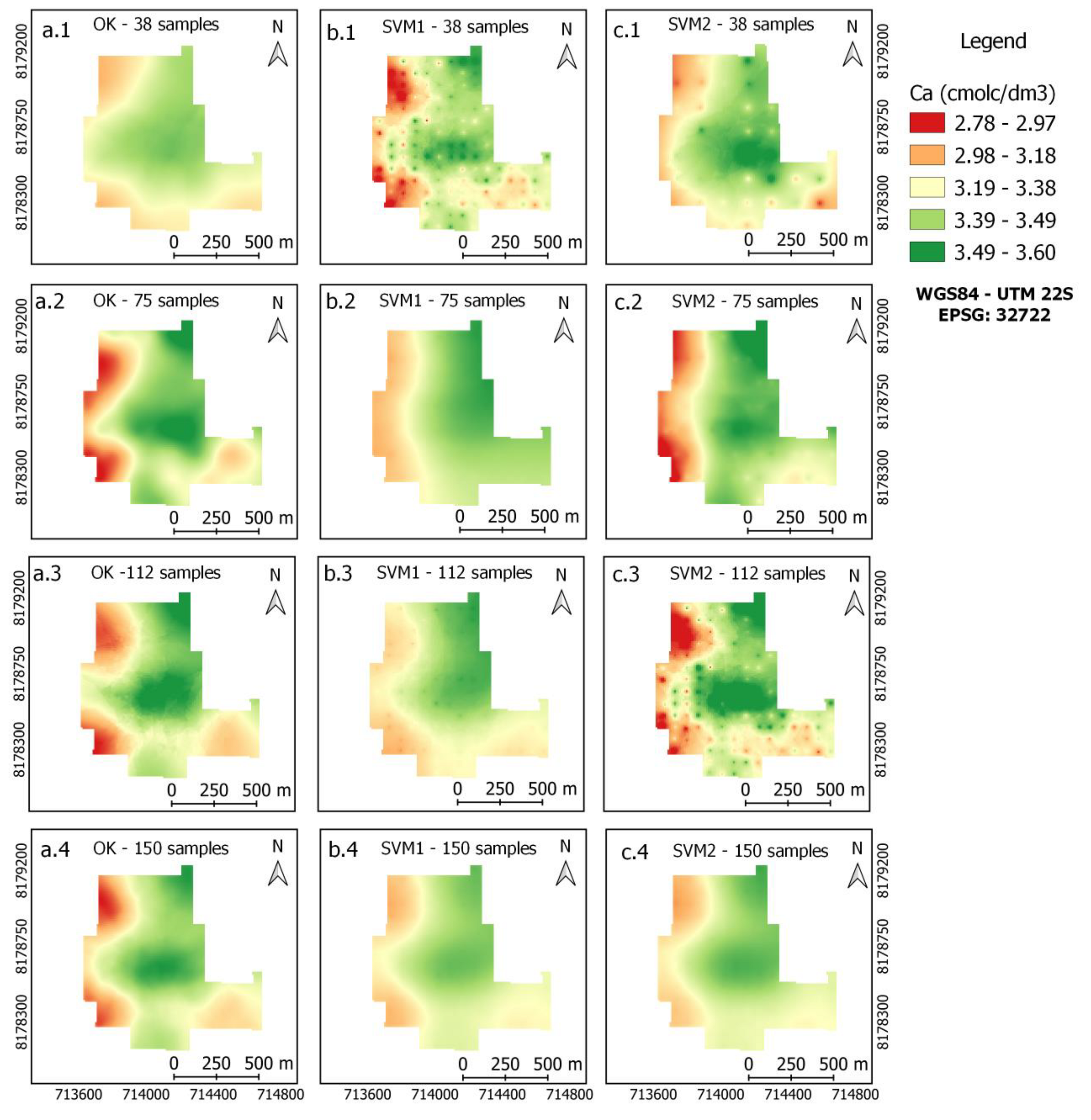
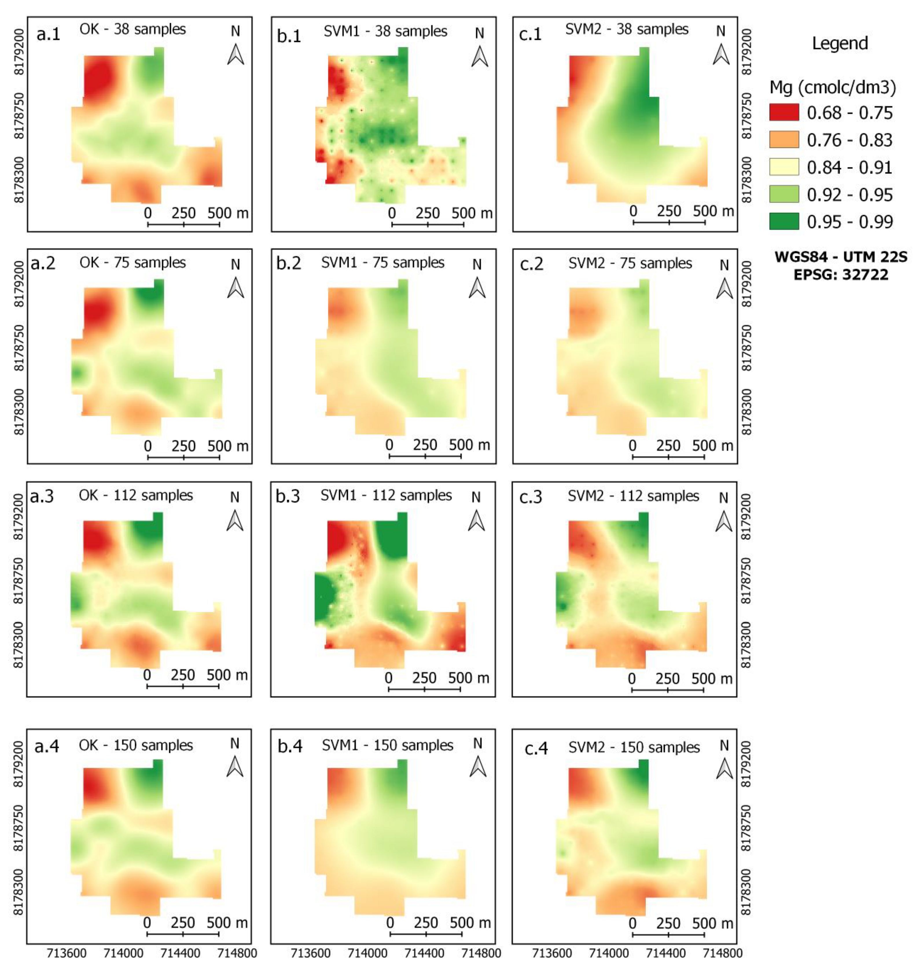
3.3. Maps of Soil Attributes

The maps of soil attributes were generated using the samples selected from the training sets with 38, 75, and 112 sampling points, as shown in Figure 4. The set of 150 points was also used to perform interpolation and obtain interpolated maps. The attributes P, K⁺, Ca²⁺, and Mg²⁺ were interpolated using the methods OK, SVM1, and SVM2, obtaining maps with four densities of points. To obtain the maps, a grid with 10 m × 10 m cells was used, totaling 7388 interpolated points. Each interpolated attribute showed a different pattern of spatial variability (Figure 9, Figure 10, Figure 11 and Figure 12). This may be associated with the characteristics of mobility of the attribute in soil, relief shape, soil formation and soil management over time.

The RMSE shown in Table 3 can be interpreted as the interpolation error for each map obtained by interpolation in each density of the sampling grid and for each soil attribute. This error was calculated based on the test set, because the values of the maps obtained by interpolation of P, K⁺, Ca²⁺, and Mg²⁺ were extracted in the same places where the test points were located, thus calculating the RMSE between the value predicted by the method and the value observed in the test set.

For the maps obtained by interpolation of the P attribute in the grid with 38 sampling points of the training set (Figure 9(a.1–c.1)), the SVM2 method had the lowest error (RMSE = 3.22 mg/dm³), considering the test set of 112 points, according to Table 3. For the grid with a density of 75 sampling points in the training and test set (Figure 9(a.2–c.2)), SVM2 also had the lowest RMSE (2.74 mg/dm³), followed by SVM1 and OK (Table 3). For the grid with a density of 112 sampling points in the training set (Figure 9(a.3–c.3)) and 38 test points, the map obtained by interpolation through the SVM1 method showed the lowest RMSE (1.94 mg/dm³), followed by OK. SVM2 had the highest error (RMSE = 2.79 mg/dm³). For the map obtained by interpolation in the grid with 150 sampling points of the training set, it was not possible to calculate the error, since no observed points were separated for the test set. For this density, the highest P contents are distributed in the central part of the map (Figure 9(a.4–c.4)).

For the maps obtained by interpolation of the K⁺ attribute in grids with 38 (Figure 10(a.1–c.1)), 75 (Figure 10(a.2–c.2)), and 112 (Figure 10(a.3–c.3)) samples of the training set, the SVM2 method had the lowest error, followed by OK in sets with 38 and 112 points and by SVM1 in the set of 75 points (Table 3). For the map obtained by interpolation in the grid of 150 points, the highest concentrations of K⁺ are located in the east and west parts of the map (Figure 10(a.4–c.4)).

The SVM2 method obtained the lowest interpolation error in the three densities of sampling grids, followed by SVM1 and OK for the Ca²⁺ attribute, as shown in Table 3. For the grid with density of 150 sampling points, Ca²⁺ had higher values in the north and center parts of the study area (Figure 11(a.4–c.4)) for the three interpolation methods.

The Mg²⁺ attribute, as observed for Ca²⁺ and K⁺, had the lowest error for maps obtained by interpolation through the SVM2 method. In the grid of 75 sampling points for the training and test set (Figure 12(a.2–c.2)), the SVM1 and SVM2 methods obtained the same error (RMSE = 0.10 cmolc/dm³). As the R² value of SVM2 (0.47) was higher than the R² in SVM1 (0.41) according to Figure 8, implying that the performance of SVM2 was better than that of SVM1. The same occurred for the grid with 38 points of the training set (Figure 12(a.1–c.1)) and the grid with 112 samples in the test set, as the error of the OK and SVM1 methods was 0.11 cmolc/dm³. OK was superior because it had higher R² values (Figure 8). For the grid with 150 sampling points, the map obtained by interpolation showed spatial behavior with the highest values concentrated in the northern part of the area (Figure 12(a.4–c.4)).

3.4. Limitations and Future Developments

Smart-Map is a QGIS plugin, allowing generation of interpolated soil attribute maps. A limitation of the plugin is that the maximum number of sampling points in the input layer is limited to 1000; for grids exceeding this limit, the plugin resamples the data based on the neighborhood of the sampled points. Another limitation is that only Ordinary Kriging and Support Vector Machine methods are implemented. Although both methods allow for generation of high-quality maps covering a wide range of applications, they do not necessarily perform well in any conceivable application. In addition, to evaluate the models, only RMSE and R² metrics were used based on Leave-one-out cross-validation; however, for certain applications there are more appropriate metrics.

Future extension of the plugin comprises implementation of Co-Kriging and other Machine Learning models such as Cubist, XGBoost, and LightGBM. Techniques for selecting features that are not based on spatial correlation such as Recursive Feature Elimination (RFE) will be implemented as well. Finally, model evaluation metrics such as EAM (Mean Absolute Error), RPD (Relative Difference Percentage) and cross-validation techniques such as K-fold and Holdout will be implemented.

4. Conclusions

Techniques for digital mapping of soil attributes were implemented using Ordinary Kriging (OK) and the Machine Learning (ML) Support Vector Machine (SVM) algorithm coded in a Smart-Map plugin for QGIS. Machine Learning interpolation allowed data from the QGIS database layers of raster- and vector-type to be used as covariates in the interpolation. The maps generated by the plugin can be exported to QGIS in a shapefile and/or raster format.

In a case study used to evaluate the performance of the Smart-Map plugin, interpolation was compared using three methods being Ordinary Kriging (OK), a machine learning Support Vector Machine method that uses the attribute itself interpolated by Inverse Distance Weighting (IDW) as covariate (SVM1), and with the use of covariates (SVM2). Conclusions are as follows:

(1)

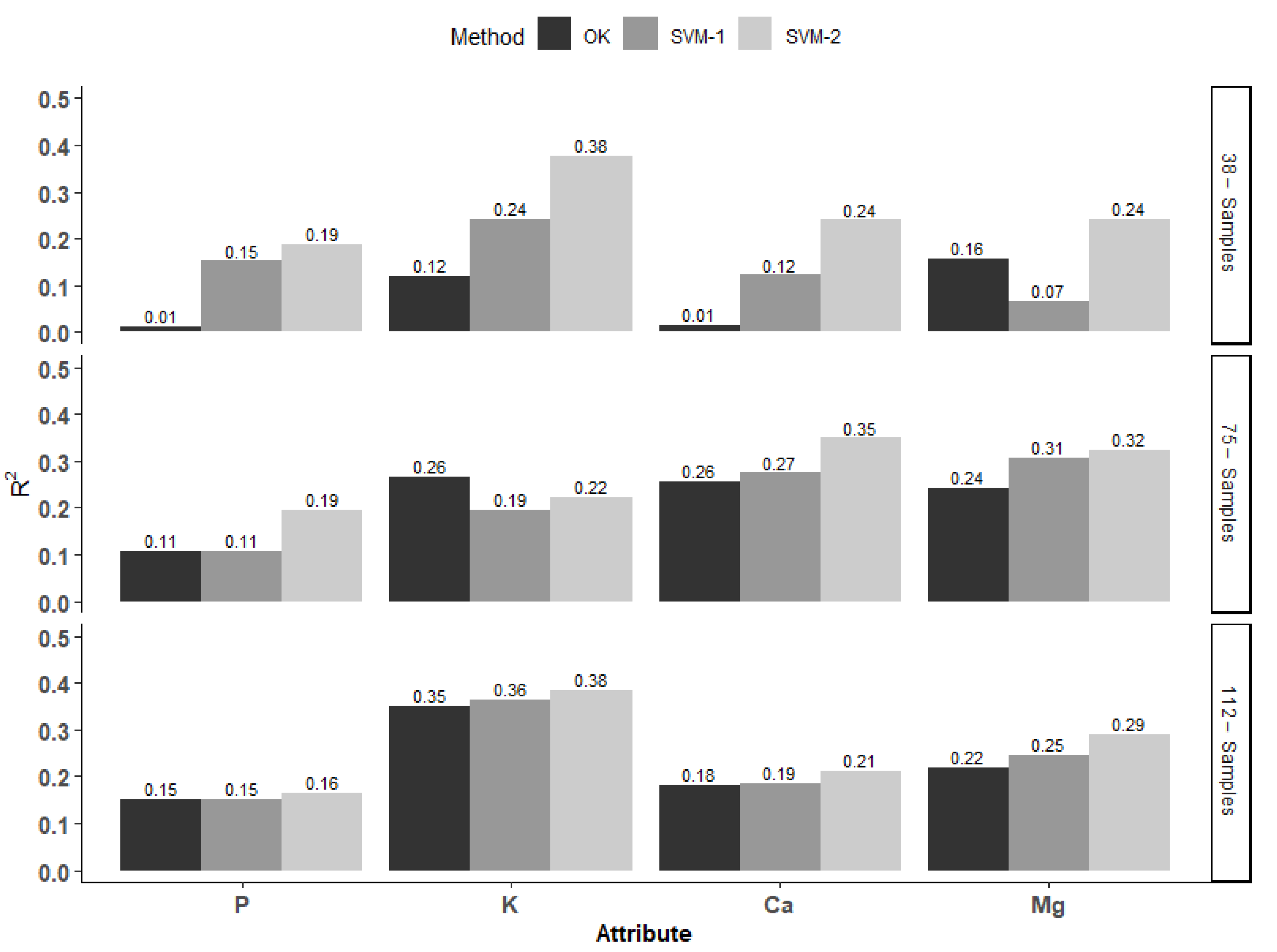
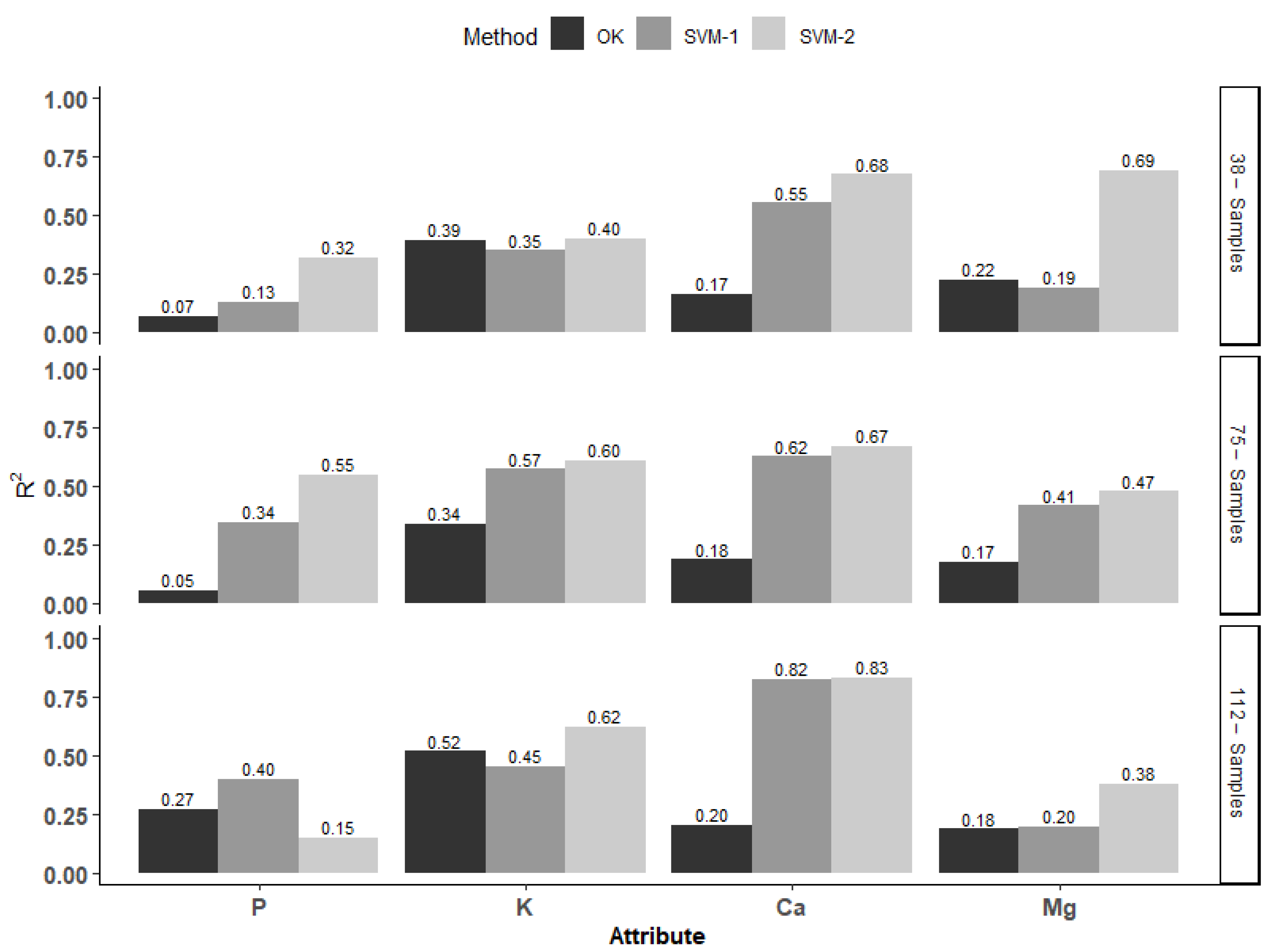
The SVM2 method was superior to other models in the prediction of soil chemical attributes for the three densities of points in the sampling grids. The R² values were higher in 11 of the 12 combinations among the four soil attributes interpolated in three densities of points of the sampling grids, considering the training set.

(2)

Considering the RMSE of the test set, SVM2 had the lowest error for the prediction of maps obtained by interpolation for the four soil attributes in the three sampling densities, except for the P attribute in the SVM1 method with a grid of 38 points in the test set.

(3)

One difficulty encountered by ML algorithms for problems of mapping and prediction of soil attributes is to handle the excessive number of covariates in the model. Spatial correlation of I’Moran proved to be efficient for the selection of covariates of greater importance in the model.

(4)

In areas with low spatial correlation of soil attributes and few sampled points, ML techniques are an alternative to the OK method, especially when covariates with a higher number of points and a significant level of correlation with the variables to be interpolated are available. The results in this study confirmed the feasibility and applicability of ML techniques, especially the “Support Vector Machine” method, for prediction and mapping of soil chemical attributes on a regional scale.

(5)

The developed Smart-Map plugin is available for download on the GitHub website. Available online: https://github.com/gustavowillam/SmartMapPlugin (accessed on 25 May 2022) and in the QGIS plugin repository Available online: https://plugins.qgis.org/plugins/Smart_Map (accessed on 25 May 2022). With a user-friendly and easy-to-use interface, Smart-Map has over 15,000 downloads according to the QGIS plugin repository. Information on how to use and obtain the software can be found in the “Supplementary Materials” section.

References

1. Malla, R.; Shrestha, S.; Khadka, D.; Bam, C.R. Soil fertility mapping and assessment of the spatial distribution of Sarlahi district, Nepal. Am. J. Agric. Sci. 2020, 7, 8–16. [Google Scholar]
2. Veronesi, F.; Schillaci, C. Comparison between geostatistical and machine learning models as predictors of topsoil organic carbon with a focus on local uncertainty estimation. Ecol. Indic. 2019, 101, 1032–1044. [Google Scholar] [CrossRef]
3. Pouladi, N.; Møller, A.B.; Tabatabai, S.; Greve, M.H. Mapping soil organic matter contents at field level with cubist, random forest and kriging. Geoderma 2019, 342, 85–92. [Google Scholar] [CrossRef]
4. Webster, R.; Oliver, M.A. Sample adequately to estimate variograms of soil properties. J. Soil Sci. 1992, 43, 177–192. [Google Scholar] [CrossRef]
5. da Matta Campbell, P.M.; Francelino, M.R.; Filho, E.I.F.; de Azevedo Rocha, P.; de Azevedo, B.C. Digital mapping of soil attributes using machine learning. Rev. Cienc. Agron. 2019, 50, 519–528. [Google Scholar] [CrossRef]
6. Guo, P.T.; Li, M.F.; Luo, W.; Tang, Q.F.; Liu, Z.W.; Lin, Z.M. Digital mapping of soil organic matter for rubber plantation at regional scale: An application of random forest plus residuals kriging approach. Geoderma 2015, 237–238, 49–59. [Google Scholar] [CrossRef]
7. Hengl, T.; Nussbaum, M.; Wright, M.N.; Heuvelink, G.B.M.; Gräler, B. Random forest as a generic framework for predictive modeling of spatial and spatio-temporal variables. PeerJ 2018, 6, e5518. [Google Scholar] [CrossRef] [Green Version]
8. Heung, B.; Ho, H.C.; Zhang, J.; Knudby, A.; Bulmer, C.E.; Schmidt, M.G. An overview and comparison of machine-learning techniques for classification purposes in digital soil mapping. Geoderma 2016, 265, 62–77. [Google Scholar] [CrossRef]
9. Sekulić, A.; Kilibarda, M.; Heuvelink, G.B.M.; Nikolić, M.; Bajat, B. Random forest spatial interpolation. Remote Sens. 2020, 12, 1–29. [Google Scholar] [CrossRef]
10. Khaledian, Y.; Miller, B.A. Selecting appropriate machine learning methods for digital soil mapping. Appl. Math. Model. 2020, 81, 401–418. [Google Scholar] [CrossRef]
11. Liakos, K.G.; Busato, P.; Moshou, D.; Pearson, S.; Bochtis, D. Machine learning in agriculture: A review. Sensors 2018, 18, 1–29. [Google Scholar] [CrossRef] [PubMed] [Green Version]
12. Meier, M.; de Souza, E.; Francelino, M.R.; Fernandes Filho, E.I.; Schaefer, C.E.G.R. Digital soil mapping using machine learning algorithms in a tropical mountainous area. Rev. Bras. de Ciência do Solo 2018, 42, 1–22. [Google Scholar] [CrossRef] [Green Version]
13. Parmley, K.A.; Higgins, R.H.; Ganapathysubramanian, B.; Sarkar, S.; Singh, A.K. Machine learning approach for prescriptive plant breeding. Sci. Rep. 2019, 9, 17132. [Google Scholar] [CrossRef] [PubMed]
14. R Core Team. R: A Language and Environment for Statistical Computing; R Foundation for Statistical Computing: Vienna, Austria, 2020; Available online: http://www.r-project.org/ (accessed on 25 May 2022).
15. Gomes, L.C.; Faria, R.M.; de Souza, E.; Veloso, G.V.; Schaefer, C.E.G.R.; Filho, E.I.F. Modelling and mapping soil organic carbon stocks in Brazil. Geoderma 2019, 340, 337–350. [Google Scholar] [CrossRef]
16. Gregorutti, B.; Michel, B.; Saint-Pierre, P. Correlation and variable importance in random forests. Stat. Comput. 2017, 27, 659–678. [Google Scholar] [CrossRef] [Green Version]
17. QGIS Development Team QGIS Geographic Information System. Open Source Geospatial Foundation Project. Available online: http://qgis.org (accessed on 25 May 2020).
18. Whelan, B.M.; McBratney, A.B.; Minasny, B. VESPER 1.5-spatial prediction software for precision agriculture. In Proceedings of the 6th International Conference on Precision on Agriculture ASA/CSSA/SSSA, Madison, WI, USA, 14–17 July 2002; Volume 179, pp. 1–14. [Google Scholar]
19. Remy, N.; Boucher, A.; Wu, J. Applied Geostatistics with SGeMS: A User’s Guide; Cambridge University Press: Cambridge, UK, 2009. [Google Scholar] [CrossRef]
20. Coelho, A.L.F.; Queiroz, D.M.; Valente, D.S.M.; Pinto, F.D.A.D.C. An open-source spatial analysis system for embedded systems. Comput. Electron. Agric. 2018, 154, 289–295. [Google Scholar] [CrossRef]
21. Valente, D.S.M.; Queiroz, D.M.; Pinto, F.D.A.D.C.; Santos, N.T.; Santos, F.L. Definition of management zones in coffee production fields based on apparent soil electrical conductivity. Sci. Agric. 2012, 69, 173–179. [Google Scholar] [CrossRef] [Green Version]
22. Isaaks, E.H.; Srivastava, R.M. An Introduction to Applied Geostatistics; Oxford University Press: New York, NY, USA, 1989. [Google Scholar]
23. Zhou, X.; Zhang, X.; Wang, B. Online support vector machine: A survey. Adv. Intell. Syst. Comput. 2016, 382, 269–278. [Google Scholar] [CrossRef]
24. Karamizadeh, S.; Abdullah, S.M.; Halimi, M.; Shayan, J.; Rajabi, M.J. Advantage and drawback of support vector machine functionality. In Proceedings of the 2014 International Conference on Computer, Communications and Control Technology (I4CT), Langkawi, Malaysia, 2–4 September 2014; pp. 63–65. [Google Scholar] [CrossRef]
25. Keskin, H.; Grunwald, S.; Harris, W.G. Digital mapping of soil carbon fractions with machine learning. Geoderma 2019, 339, 40–58. [Google Scholar] [CrossRef]
26. Xu, S.; Zhao, Y.; Wang, M.; Shi, X. Comparison of multivariate methods for estimating selected soil properties from intact soil cores of paddy fields by Vis–NIR spectroscopy. Geoderma 2018, 310, 29–43. [Google Scholar] [CrossRef]
27. Bezdek, J.C.; Ehrlich, R.; Full, W. FCM: The fuzzy c-means clustering algorithm. Comput. Geosci. 1984, 10, 191–203. [Google Scholar] [CrossRef]
28. Albornoz, E.M.; Kemerer, A.C.; Galarza, R.; Mastaglia, N.; Melchiori, R.; Martínez, C.E. Development and evaluation of an automatic software for management zone delineation. Precis. Agric. 2018, 19, 463–476. [Google Scholar] [CrossRef]
29. Chen, S.; Wang, S.; Shukla, M.K.; Wu, D.; Guo, X.; Li, D.; Du, T. Delineation of management zones and optimization of irrigation scheduling to improve irrigation water productivity and revenue in a farmland of northwest China. Precis. Agric. 2019, 21, 655–677. [Google Scholar] [CrossRef]
30. Warner, J.; Sexauer, J.; Unnikrishnan, A. JDWarner/Scikit-Fuzzy: Scikit-Fuzzy, Version 0.4.2. Available online: https://scikit-fuzzy.github.io/scikit-fuzzy/ (accessed on 18 July 2019).
31. WRB-IUSS World Reference Base for Soil Resources 2014, update 2015: International soil classification system for naming soils and creating legends for soil maps. World Soil Resource. Report. 2015, 106, 1–191.
32. Calamita, G.; Brocca, L.; Perrone, A.; Piscitelli, S.; Lapenna, V.; Melone, F.; Moramarco, T. Electrical resistivity and TDR methods for soil moisture estimation in Central Italy Test-Sites. J. Hydrol. 2012, 454–455, 101–112. [Google Scholar] [CrossRef]
33. Costa, M.M.; de Queiroz, D.M.; Pinto, F.D.A.D.C.; dos Reis, E.F.; Santos, N.T. Moisture content effect in the relationship between apparent electrical conductivity and soil attributes. Acta Sci. Agron. 2014, 36, 395–401. [Google Scholar] [CrossRef] [Green Version]
34. Muphy, B.; Mullher, S.; Yurchark, R. GeoStat-Framework/PyKrige, Version v1.5.1. Available online: https://github.com/GeoStat-Framework/PyKrige (accessed on 8 January 2020).
35. Pedregosa, F.; Varoquaux, G.; Granfort, A.; Michel, V.; Thirion, B. Scikit-Learn: Machine learning in python. J. Mach. Learn. Res. 2011, 12, 2825–2830. [Google Scholar] [CrossRef]
36. Huo, X.-N.; Li, H.; Sun, D.-F.; Zhou, L.-D.; Li, B.-G. Combining geostatistics with Moran’s i analysis for mapping soil heavy metals in Beijing, China. Int. J. Environ. Res. Public Health 2012, 9, 995–1017. [Google Scholar] [CrossRef] [Green Version]
37. Pereira, G.W.; Valente, D.S.M.; de Queiroz, D.M.; Santos, N.T.; Fernandes-Filho, E.I. Soil mapping for precision agriculture using support vector machines combined with inverse distance weighting. Precis. Agric. 2022, 23. [Google Scholar] [CrossRef]
38. Liu, Q.; Xie, W.J.; Xia, J.B. Using semivariogram and Moran’s i techniques to evaluate spatial distribution of soil micronutrients. Commun. Soil Sci. Plant Anal. 2013, 44, 1182–1192. [Google Scholar] [CrossRef]
39. Legendre, P.; Fortin, M.-J. Spatial pattern and ecological analysis. Vegetatio 1989, 80, 107–138. [Google Scholar] [CrossRef]
40. Lee, S. Developing a bivariate spatial association measure: An integration of Pearson’s r and Moran’s i. Geogr. Syst. 2001, 3, 369–385. [Google Scholar] [CrossRef]
41. Rey, S.J.; Anselin, L. PySAL: A Python Library of Spatial Analytical Methods; Fischer, M., Getis, A., Eds.; Springer: Berlin/Heidelberg, Germany, 2010. [Google Scholar]
42. Celisse, A.; Robin, S. Nonparametric density estimation by exact leave-p-out cross-validation. Comput. Stat. Data Anal. 2008, 52, 2350–2368. [Google Scholar] [CrossRef]
43. Cawley, G.C.; Talbot, N.L.C. Efficient leave-one-out cross-validation of kernel fisher discriminant classifiers. Pattern Recognit. 2003, 36, 2585–2592. [Google Scholar] [CrossRef]
Figure 1. Flowchart of the main processing steps of Smart-Map.
Agronomy 12 01350 g001
Figure 2. Graphical User Interface of Smart-Map. (a) Interpolation by OK. (b) Interpolation by SVM.
Agronomy 12 01350 g002
Figure 3. Geographical location of the study area and distribution of sampling points in Anápolis/Goianápolis, Goiás, Brazil.
Agronomy 12 01350 g003
Figure 4. Number of sampling points in: (a) original grid with 150 points; (b) 38 points for training and 112 points for testing; (c) 75 points for training and 75 points for testing; (d) 112 points for training and 38 points for testing.
Agronomy 12 01350 g004
Figure 5. Construction of the ML model. (a) Selection of the 16 closest neighbors to the point where the user wishes to estimate the attribute value using the IDW method. (b) Definition of the ML model (Train_Features) for the methods SVM1 and SVM2: features (X matrix) and target (y vector). (c) SVM model trained for the methods SVM1 and SVM2. (d) Map interpolated from the test set.
Agronomy 12 01350 g005
Figure 6. Univariate Global Moran’s Index for the soil attributes P, K+, Ca2+, and Mg2+ and bivariate Moran’s Index among soil attributes P, K+, Ca2+, and Mg2+ and covariates for the sampling grids of the training set with: (a) 38 points; (b) 75 points; (c) 112 points. *, ** indicating significance at 0.05 and 0.01 levels, respectively. *** covariates were used by the SVM2 method to interpolate the soil attributes P, K+, Ca2+, and Mg2+.
Agronomy 12 01350 g006
Figure 7. Coefficient of Determination (R2) calculated for the attributes P, K+, Ca2+, and Mg2+ among three sampling grids for the training set.
Agronomy 12 01350 g007
Figure 8. Coefficient of Determination (R2) calculated for the attributes P, K+, Ca2+, and Mg2+ among three sampling grids for the test set.
Agronomy 12 01350 g008
Figure 9. Maps obtained by interpolation of Phosphorus (P): (a) OK, (b) SVM1, (c) SVM2; Set of points (training): 38 (a.1c.1), 75 (a.2c.2), 112 (a.3c.3), and 150 points (a.4c.4).
Agronomy 12 01350 g009
Figure 10. Maps obtained by interpolation of Potassium (K+): (a) OK, (b) SVM1, (c) SVM2; Set of points (training): 38 (a.1c.1), 75 (a.2c.2), 112 points (a.3c.3), and 150 points (a.4c.4).
Agronomy 12 01350 g010
Figure 11. Maps obtained by interpolation of Calcium (Ca2+): (a) OK, (b) SVM1, (c) SVM2; Set of points (training): 38 (a.1c.1), 75 (a.2c.2), 112 points (a.3c.3), and 150 points (a.4c.4).
Agronomy 12 01350 g011
Figure 12. Maps obtained by interpolation of Magnesium (Mg2+): (a) OK, (b) SVM1, (c) SVM2; Set of points (training): 38 (a.1c.1), 75 (a.2c.2), 112 points (a.3c.3), and 150 points (a.4c.4).
Agronomy 12 01350 g012