
Estimation of Genetic Variances and Stability Components of Yield-Related Traits of Green Super Rice at Multi-Environmental Conditions in Pakistan


 ,
,  ,
,
Abstract
:1. Introduction
2. Materials and Methods
2.1. Plant Material
2.2. Experimental Location
2.3. Experimental Procedures and Cultural Practices
2.4. Statistical Analysis
2.4.1. Analysis of Variance
2.4.2. Genetic Parameters
2.4.3. Estimation of Stability Parameters
2.4.4. Univariate Stability Analysis
2.4.5. Multivariate Stability Analysis
2.4.6. Additive Main Effect and Multiplicative Interaction (AMMI) Model
2.4.7. Biplot Analysis
3. Results
3.1. Combined Analysis of Variance
3.2. Analysis of Genetic and Phenotypic Variances
3.3. Univariate Models
3.3.1. Univariate Parametric Stability Statistics (First-Year 2020)
3.3.2. Univariate Parametric Stability Statistics (Second-Year 2021)
3.4. Multivariate Models
3.4.1. AMMI Analysis of Variance (First-Year 2020)
3.4.2. AMMI Analysis of Variance (Second-Year 2021)
3.4.3. GGE Biplot Analysis (First-Year 2020)
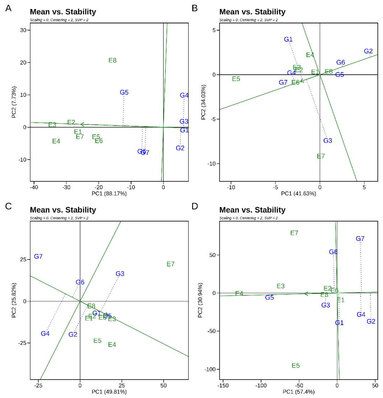
‘Mean vs. Stability’ Analysis of GGE Biplot
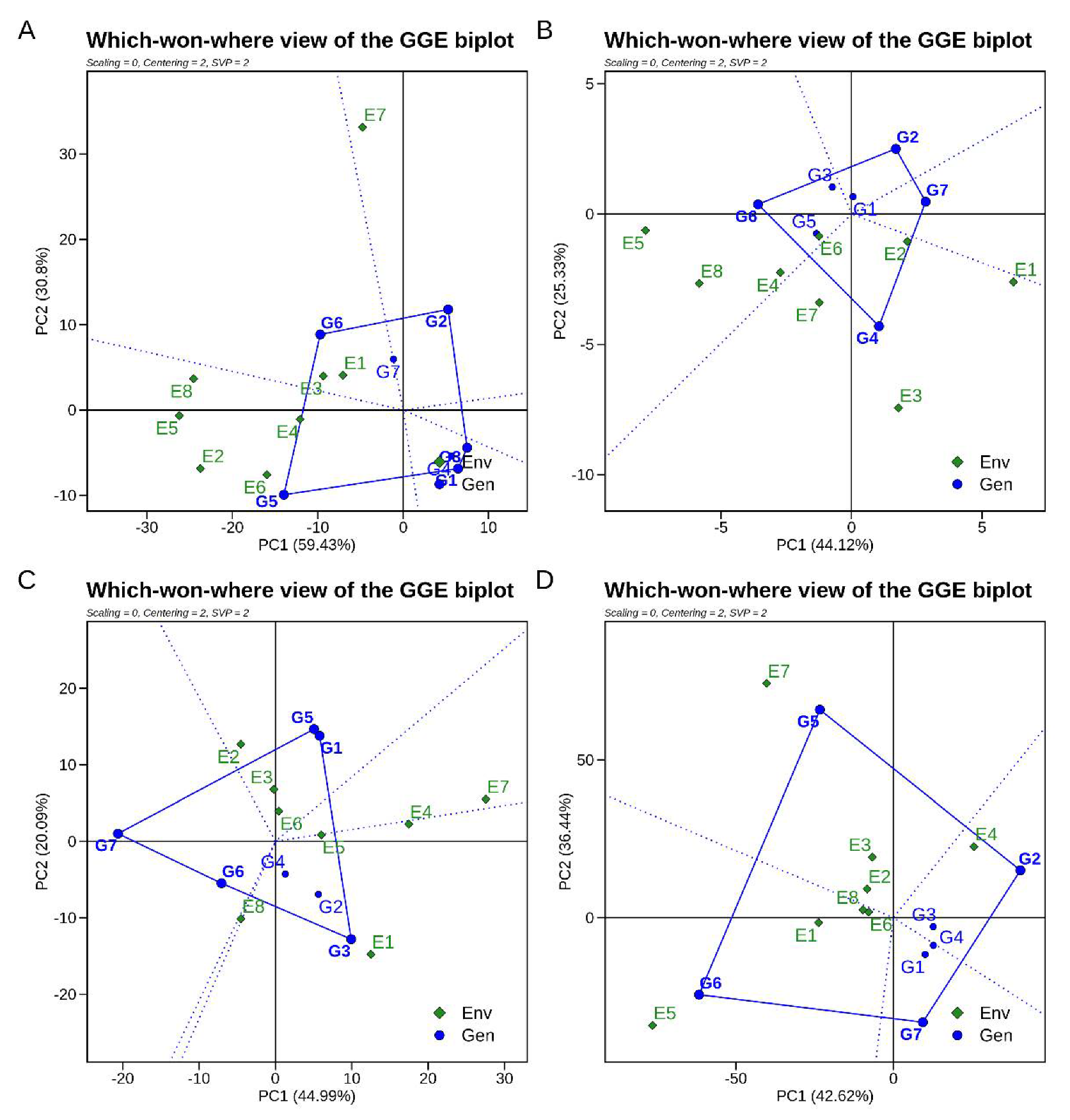
‘Which-Won-Where’ GGE Biplot
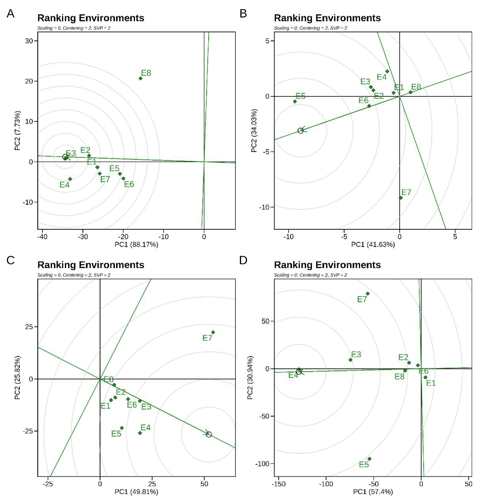
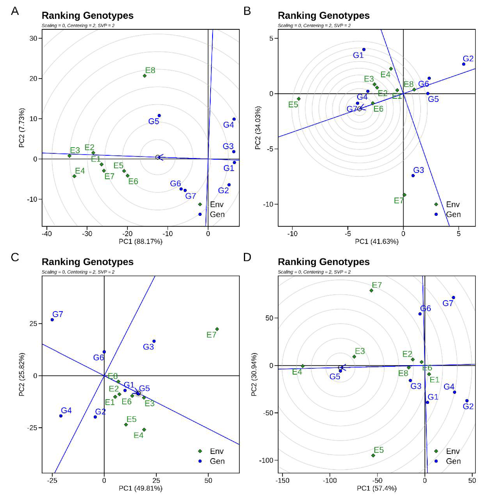
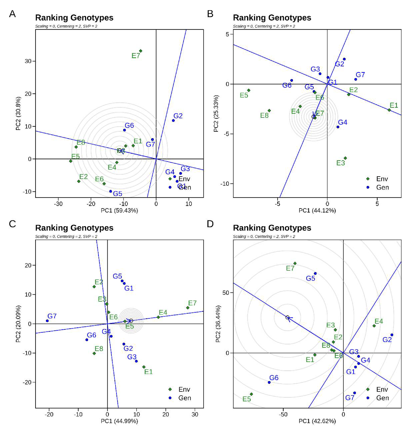
Locations and Genotypes Ranking: Best and Stable Location/Genotypes Evaluation
3.4.4. GGE Biplot Analysis (Second-Year 2021)
Mean vs. Stability’ Analysis of GGE Biplot (First-Year 2021)
‘Which-Won-Where’ GGE Biplot
Locations and Genotypes Ranking: Best and Stable Location/Genotypes Evaluation
4. Discussion
5. Conclusions
Supplementary Materials
Author Contributions
Funding
Data Availability Statement
Acknowledgments
Conflicts of Interest
References
- FAO. World Food and Agriculture—Statistical Yearbook 2020; FAO Statistical Yearbook—World Food and Agriculture; FAO: Rome, Italy, 2020; ISBN 978-92-5-133394-5. [Google Scholar]
- Yu, S.; Ali, J.; Zhang, C.; Li, Z.; Zhang, Q. Genomic Breeding of Green Super Rice Varieties and Their Deployment in Asia and Africa. Theor. Appl. Genet. 2020, 133, 1427–1442. [Google Scholar] [CrossRef] [PubMed] [Green Version]
- Wricke, G. Uber eine Methode zur Erfassung der okologischen Streubreite in Feldverzuchen. Z. Pflanzenzuchtg 1962, 47, 92–96. [Google Scholar]
- Piepho, H.P. A Comparison of the Ecovalence and the Variance of Relative Yield as Measures of Stability. J. Agron. Crop Sci. 1994, 173, 1–4. [Google Scholar] [CrossRef]
- Farshadfar, E.; Mohammadi, R.; Aghaee, M.; Vaisi, Z. GGE biplot analysis of genotype x environment interaction in wheat-barley disomic addition lines. Aust. J. Crop Sci. 2012, 6, 1074–1079. [Google Scholar] [CrossRef]
- Shukla, G. Some statistical aspects of partitioning genotype environmental components of variability. Heredity 1972, 29, 237–245. [Google Scholar] [CrossRef]
- Francis, T.R.; Kannenberg, L.W. Yield stability studies in short-season maize. i. a descriptive method for grouping genotypes. Can. J. Plant Sci. 1978, 58, 1029–1034. [Google Scholar] [CrossRef]
- Roemer, J. Sinde die ertagdreichen Sorten ertagissicherer. Mitt DLG 1917, 32, 87–89. [Google Scholar]
- Plaisted, R.L.; Peterson, L.C. A technique for evaluating the ability of selections to yield consistently in different locations or seasons. Am. Potato J. 1959, 36, 381–385. [Google Scholar] [CrossRef]
- Plaisted, R.L. A shorter method for evaluating the ability of selections to yield consistently over locations. Am. Potato J. 1960, 37, 166–172. [Google Scholar] [CrossRef]
- Finlay, K.W.; Wilkinson, G.N. The analysis of adaptation in a plant-breeding programme. Aust. J. Agric. Res. 1963, 14, 742–754. [Google Scholar] [CrossRef] [Green Version]
- Gauch, H.G., Jr. Model selection and validation for yield trials with interaction. Biometrics 1988, 44, 705–715. [Google Scholar] [CrossRef]
- Yan, W.; Cornelius, P.L.; Crossa, J.; Hunt, L.A. Two Types of GGE Biplots for Analyzing Multi-Environment Trial Data. Crop Sci. 2001, 41, 656–663. [Google Scholar] [CrossRef] [Green Version]
- Gauch, H.G., Jr.; Piepho, H.-P.; Annicchiarico, P. Statistical Analysis of Yield Trials by AMMI and GGE: Further Considerations. Crop Sci. 2008, 48, 866–889. [Google Scholar] [CrossRef]
- Nassar, R.; Hühn, M. Studies on Estimation of Phenotypic Stability: Tests of Significance for Nonparametric Measures of Phenotypic Stability. Biometrics 1987, 43, 45–53. [Google Scholar] [CrossRef]
- Kang, M. A rank-sum method for selecting high-yielding, stable corn genotypes. Cereal Res. Commun. 1988, 16, 113–115. [Google Scholar]
- Fox, P.N.; Skovmand, B.; Thompson, B.K.; Braun, H.-J.; Cormier, R. Yield and adaptation of hexaploid spring triticale. Euphytica 1990, 47, 57–64. [Google Scholar] [CrossRef]
- Thennarasu, K. On Certain Non-Parametric Procedures for Studying Genotype-Environment Inertactions and Yield Stability. Ph.D. Thesis, IARI, Division of Agricultural Statistics, New Delhi, India, 1995. [Google Scholar]
- Farshadfar, E. Incorporation of AMMI stability value and grain yield in a single non-parametric index (GSI) in bread wheat. Pak. J. Biol. Sci. PJBS 2008, 11, 1791–1796. [Google Scholar] [CrossRef] [Green Version]
- Burton, G.W.; DeVane, E.H. Estimating Heritability in Tall Fescue (Festuca Arundinacea) from Replicated Clonal Material1. Agron. J. 1953, 45, 478–481. [Google Scholar] [CrossRef]
- Purchase, J.L.; Hatting, H.; van Deventer, C.S. Genotype × environment interaction of winter wheat (Triticum aestivum L.) in South Africa: II. Stability analysis of yield performance. South Afr. J. Plant Soil 2000, 17, 101–107. [Google Scholar] [CrossRef]
- Jambhulkar, N.; Rath, N.; Bose, L.; Subudhi, H.; Mondal, B.; Das, L.; Meher, J. Stability analysis for grain yield in rice in demonstrations conducted during rabi season in India. ORYZA Int. J. Rice 2017, 54, 234. [Google Scholar] [CrossRef]
- Zobel, R.W.; Wright, M.J.; Gauch, H.G., Jr. Statistical Analysis of a Yield Trial. Agron. J. 1988, 80, 388–393. [Google Scholar] [CrossRef]
- Olivoto, T.; Lúcio, A.D. metan: An R package for multi-environment trial analysis. Methods Ecol. Evol. 2020, 11, 783–789. [Google Scholar] [CrossRef]
- Kempton, R.A. The use of biplots in interpreting variety by environment interactions. J. Agric. Sci. 1984, 103, 123–135. [Google Scholar] [CrossRef]
- Gauch, H.G., Jr.; Zobel, R.W. Optimal Replication in Selection Experiments. Crop Sci. 1996, 36, 838–843. [Google Scholar] [CrossRef]
- Oladosu, Y.; Rafii, M.Y.; Abdullah, N.; Magaji, U.; Miah, G.; Hussin, G.; Ramli, A. Genotype × Environment interaction and stability analyses of yield and yield components of established and mutant rice genotypes tested in multiple locations in Malaysia. Acta Agric. Scand. Sect. B Soil Plant Sci. 2017, 67, 590–606. [Google Scholar] [CrossRef]
- Haider, Z.; Akhter, M.; Mahmood, A.; Khan, R.A.R. Comparison of GGE biplot and AMMI analysis of multi-environment trial (MET) data to assess adaptability and stability of rice genotypes. Afr. J. Agric. Res. 2017, 12, 3542–3548. [Google Scholar] [CrossRef] [Green Version]
- Bose, L.; Jambhulkar, N.; Singh, O. Additive Main effects and Multiplicative Interaction (AMMI) analysis of grain yield stability in early duration rice. JAPS J. Anim. Plant Sci. 2014, 24, 1885–1897. [Google Scholar]
- Zeigler, R.S. Rice research for poverty alleviation and environmental sustainability in Asia. GeoJournal 2006, 35, 286–298. [Google Scholar]
- Kanfany, G.; Ayenan, M.A.T.; Zoclanclounon, Y.A.B.; Kane, T.; Ndiaye, M.; Diatta, C.; Diatta, J.; Gueye, T.; Fofana, A. Analysis of Genotype-Environment Interaction and Yield Stability of Introduced Upland Rice in the Groundnut Basin Agroclimatic Zone of Senegal. Adv. Agric. 2021, 2021, e4156167. [Google Scholar] [CrossRef]
- Balakrishnan, D.; Subrahmanyam, D.; Badri, J.; Raju, A.K.; Rao, Y.V.; Beerelli, K.; Mesapogu, S.; Surapaneni, M.; Ponnuswamy, R.; Padmavathi, G.; et al. Genotype × Environment Interactions of Yield Traits in Backcross Introgression Lines Derived from Oryza sativa cv. Swarna/Oryza nivara. Front. Plant Sci. 2016, 7, 1530. [Google Scholar] [CrossRef] [Green Version]
- Sharifi, P.; Aminpanah, H.; Erfani, R.; Mohaddesi, A.; Abbasian, A. Evaluation of Genotype × Environment Interaction in Rice Based on AMMI Model in Iran. Rice Sci. 2017, 24, 173–180. [Google Scholar] [CrossRef]
- Shrestha, J.; Kushwaha, U.K.S.; Maharjan, B.; Kandel, M.; Gurung, S.B.; Poudel, A.P.; Karna, M.K.L.; Acharya, R. Grain Yield Stability of Rice Genotypes. Indones. J. Agric. Res. 2020, 3, 116–126. [Google Scholar] [CrossRef]
- Shojaei, S.H.; Mostafavi, K.; Omrani, A.; Omrani, S.; Nasir Mousavi, S.M.; Illés, Á.; Bojtor, C.; Nagy, J. Yield Stability Analysis of Maize (Zea mays L.) Hybrids Using Parametric and AMMI Methods. Scientifica 2021, 2021, 5576691. [Google Scholar] [CrossRef] [PubMed]
- Tremmel-Bede, K.; Szentmiklóssy, M.; Tömösközi, S.; Török, K.; Lovegrove, A.; Shewry, P.R.; Láng, L.; Bedő, Z.; Vida, G.; Rakszegi, M. Stability analysis of wheat lines with increased level of arabinoxylan. PLoS ONE 2020, 15, e0232892. [Google Scholar] [CrossRef] [PubMed]
- Pour-Aboughadareh, A.; Khalili, M.; Poczai, P.; Olivoto, T. Stability Indices to Deciphering the Genotype-by-Environment Interaction (GEI) Effect: An Applicable Review for Use in Plant Breeding Programs. Plants 2022, 11, 414. [Google Scholar] [CrossRef] [PubMed]
- Katsura, K.; Tsujimoto, Y.; Oda, M.; Matsushima, K.; Inusah, B.; Dogbe, W.; Sakagami, J.-I. Genotype-by-environment interaction analysis of rice (Oryza spp.) yield in a floodplain ecosystem in West Africa. Eur. J. Agron. 2016, 73, 152–159. [Google Scholar] [CrossRef]
- Gauch, H.G.J. AMMI analysis on yield trials. CIMMYT Wheat Spec. Rep. CIMMYT 1992, 9–12. [Google Scholar]
- Wade, L.J.; McLaren, C.G.; Quintana, L.; Harnpichitvitaya, D.; Rajatasereekul, S.; Sarawgi, A.K.; Kumar, A.; Ahmed, H.U.; Sarwoto; Singh, A.K.; et al. Genotype by environment interactions across diverse rainfed lowland rice environments. Field Crops Res. 1999, 64, 35–50. [Google Scholar] [CrossRef]
- Singh, R.; Huerta Espino, J. The use of single-backcross, selected-bulk breeding approach for transferring minor genes based rust resistance into adapted cultivars. Cereals 2004, 54, 48–51. [Google Scholar]


| Genotypes with Codes | Locations with Environment Codes | Years |
|---|---|---|
| GSR-48 = G1 | Pindi Bhattian = E1 | 2020, 2021 |
| GSR-82 = G2 | Kala Shah Kaku = E2 | |
| GSR-112 = G3 | Narowal = E3 | |
| GSR-252 = G4 | Swat = E4 | |
| GSR-305 = G5 | Islamabad = E5 | |
| IRRI6 = G6 | Dera Ismail Khan = E6 | |
| Kissan Basmati = G7 | Muzaffargarh = E7 | |
| Dokri = E8 |
| Locations | Month | July | August | September | October | November | Soil Type | |||||
|---|---|---|---|---|---|---|---|---|---|---|---|---|
| Year | Temp (°C) | Rain (mm) | Temp (°C) | Rain (mm) | Temp (°C) | Rain (mm) | Temp (°C) | Rain (mm) | Temp (°C) | Rain (mm) | ||
| NARC | 2020 | 35 | 162.5 | 32 | 165.1 | 31 | 68.5 | 29 | 22.8 | 22 | 12.7 | loam |
| 2021 | 28 | 174 | 26 | 162 | 25 | 73 | 21 | 31 | 15 | 39 | ||
| Swat | 2020 | 33 | 89.8 | 35 | 55.8 | 28 | 91.8 | 23 | 36.8 | 19 | 64.4 | sandy |
| 2021 | 28 | 55.8 | 27 | 55.8 | 25 | 27.9 | 19 | 20.3 | 13 | 15.2 | ||
| Kala Shah Kaku | 2020 | 36 | 50.6 | 33 | 57.2 | 32 | 39.2 | 32 | 3.2 | 23.5 | 2.8 | silty clay |
| 2021 | 31 | 134.6 | 31 | 124.4 | 30 | 55.8 | 25 | 12.7 | 20 | 5 | ||
| Pindi Bhattian | 2020 | 34 | 71.1 | 33 | 67.5 | 32 | 45.3 | 32 | 6.4 | 24 | 4.4 | sandy loam |
| 2021 | 35 | 19.2 | 36 | 91.4 | 34 | 40.6 | 30 | 7.6 | 24 | 5 | ||
| Narowal | 2020 | 36 | 160.5 | 33 | 232.6 | 35 | 139.9 | 32 | 14.3 | 23.5 | 12.4 | silty, loamy |
| 2021 | 33 | 89 | 31 | 59 | 28.5 | 43 | 23 | 11 | 19 | 4 | ||
| Muzaffargarh | 2020 | 40 | 37.5 | 37 | 43.7 | 36 | 20.8 | 36 | 2.21 | 28.5 | 1.8 | salinity |
| 2021 | 39.2 | 52 | 38.1 | 40 | 37.2 | 19 | 34.4 | 2 | 28.3 | 3 | ||
| Dokri | 2020 | 41 | 118.8 | 38.5 | 106.8 | 37 | 50.1 | 33 | 12.23 | 26.5 | 5.8 | sandy clay loam |
| 2021 | 41.1 | 41 | 39 | 24 | 38.3 | 9 | 35.7 | 2 | 30.1 | 2 | ||
| Dera Ismail Khan | 2020 | 33 | 61 | 32 | 58 | 30 | 18 | 25 | 5 | 19 | 2 | sandy/loamy sand |
| 2021 | 41.4 | 60 | 38.4 | 57 | 37.3 | 18 | 36.6 | 5 | 33.2 | 2 | ||
| Source of Variation | df | Plant Height | Tillers Per Plant | Grain Yield per plant | Straw Yield per plant |
|---|---|---|---|---|---|
| Genotype | 6 | 1.07 × 10−52 | 7.07 × 10⁻⁴ | 3.14 × 10⁻¹⁶ | 1.54 × 10⁻¹⁵ |
| location | 7 | 2.76 × 10⁻¹² | 2.12 × 10−52 | 1.05 × 10−86 | 2.74 × 10−60 |
| Year | 1 | 1.78 × 10⁻³ | 2.43 × 10⁻² | 1.52 × 10−72 | 7.03 × 10−36 |
| Replication | 2 | 7.59 × 10⁻⁶ | 6.57 × 10⁻¹ | 2.30 × 10⁻¹ | 9.54 × 10⁻³ |
| Genotype: Location | 42 | 3.78 × 10⁻⁵ | 4.77 × 10⁻³ | 1.97 × 10⁻¹⁰ | 3.23 × 10⁻⁷ |
| Genotype: Year | 6 | 1.76 × 10⁻⁶ | 6.72 × 10⁻² | 1.88 × 10⁻³ | 6.03 × 10⁻³ |
| Genotype:Location:Year | 42 | 2.84 × 10⁻⁷ | 2.22 × 10⁻³ | 4.11 × 10⁻⁶ | 3.97 × 10⁻¹⁵ |
| Genetics Parameters | Plant Height | Tillers Per Plant | Grain Yield Per Plant | Straw Yield per Plant |
|---|---|---|---|---|
| Vg | 1104.9 | 9.9 | 466 | 2468 |
| Ve | 14 | 3.2 | 28.6 | 161.2 |
| Vp | 1118 | 13.1 | 490 | 2629 |
| (%) | 98.7 | 75.3 | 94.2 | 94 |
| Year 2020 | Plant Height | Tillers per Plant | Grain Yield per Plant | Straw Yield per Plant | ||||||||||||
|---|---|---|---|---|---|---|---|---|---|---|---|---|---|---|---|---|
| Lines | Wi2 | ASV | ASI | Wi2 | ASV | ASI | Wi2 | ASV | ASI | Wi2 | ASV | ASI | ||||
| G1 | −0.6 | 63.5 | 1.5 | 0.3 | 7.3 | 126.1 | 2.7 | 0.8 | 59.9 | 1277.4 | 2.3 | 0.5 | 399.5 | 8503.5 | 4.3 | 1.7 |
| G2 | 32.9 | 568.4 | 3.5 | 0.8 | 7.9 | 135.0 | 2.0 | 0.6 | 84.0 | 1637.9 | 6.5 | 1.4 | 672.7 | 12601.5 | 6.0 | 2.4 |
| G3 | 8.7 | 204.6 | 2.9 | 0.6 | 12.0 | 196.1 | 3.5 | 1.0 | 280.5 | 4586.2 | 11.4 | 2.6 | 269.2 | 6548.4 | 2.4 | 1.0 |
| G4 | 43.6 | 727.7 | 7.8 | 1.7 | 3.5 | 68.4 | 1.2 | 0.3 | 230.7 | 3839.2 | 10.6 | 2.4 | 352.8 | 7803.6 | 4.6 | 1.8 |
| G5 | 23.3 | 423.4 | 2.2 | 0.5 | 3.9 | 74.4 | 1.0 | 0.3 | 118.8 | 2159.7 | 4.6 | 1.0 | 1598.0 | 26481.4 | 8.4 | 3.4 |
| G6 | 33.0 | 569.8 | 6.6 | 1.5 | 0.6 | 25.5 | 0.5 | 0.1 | 74.5 | 1495.7 | 3.9 | 0.8 | 931.2 | 16478.9 | 6.2 | 2.5 |
| G7 | 30.6 | 533.2 | 6.3 | 1.4 | 1.2 | 34.2 | 1.1 | 0.3 | 32.7 | 869.0 | 0.5 | 0.1 | 1633.6 | 27014.9 | 8.6 | 3.5 |
| Year 2021 | Plant height | Tillers Per Plant | Grain Yield per Plant | Straw Yield per Plant | ||||||||||||
| Lines | Wi2 | ASV | ASI | Wi2 | ASV | ASI | Wi2 | ASV | ASI | Wi2 | ASV | ASI | ||||
| G1 | 22.5 | 484.5 | 4.1 | 0.6 | 2.1 | 52.3 | 0.6 | 0.1 | 74.1 | 1272.1 | 3.5 | 0.9 | 133.1 | 3218.3 | 2.5 | 0.7 |
| G2 | 95.7 | 1582.1 | 15.6 | 2.5 | 2.8 | 61.7 | 2.2 | 0.4 | 40.4 | 766.7 | 3.4 | 0.8 | 397.0 | 7176.7 | 7.7 | 2.1 |
| G3 | 29.3 | 585.5 | 3.0 | 0.4 | 0.6 | 29 | 1.7 | 0.3 | 70.0 | 1210.7 | 5.1 | 1.3 | −10.6 | 1061.5 | 1.8 | 0.5 |
| G4 | 8.3 | 270.1 | 3.0 | 0.4 | 7.9 | 138 | 3.4 | 0.7 | −1.2 | 141.2 | 0.9 | 0.2 | 87.3 | 2531.9 | 0.8 | 0.2 |
| G5 | 136.5 | 2194.3 | 18.3 | 2.9 | 5.2 | 97.8 | 2.3 | 0.4 | 55.2 | 988.2 | 2.7 | 0.7 | 765.7 | 12707.5 | 9.0 | 2.5 |
| G6 | 25.6 | 530.2 | 4.8 | 0.7 | 14.4 | 235 | 6.1 | 1.2 | 62.5 | 1098.0 | 5.4 | 1.4 | 1012.1 | 16403.0 | 12.4 | 3.4 |
| G7 | 21.7 | 472.5 | 5.8 | 0.9 | 13 | 215 | 5.1 | 1.0 | 70.6 | 1218.6 | 6.3 | 1.6 | 465.7 | 8208.4 | 4.7 | 1.3 |
Publisher’s Note: MDPI stays neutral with regard to jurisdictional claims in published maps and institutional affiliations. |
© 2022 by the authors. Licensee MDPI, Basel, Switzerland. This article is an open access article distributed under the terms and conditions of the Creative Commons Attribution (CC BY) license (https://creativecommons.org/licenses/by/4.0/).
Share and Cite
Zaid, I.U.; Zahra, N.; Habib, M.; Naeem, M.K.; Asghar, U.; Uzair, M.; Latif, A.; Rehman, A.; Ali, G.M.; Khan, M.R. Estimation of Genetic Variances and Stability Components of Yield-Related Traits of Green Super Rice at Multi-Environmental Conditions in Pakistan. Agronomy 2022, 12, 1157. https://doi.org/10.3390/agronomy12051157
Zaid IU, Zahra N, Habib M, Naeem MK, Asghar U, Uzair M, Latif A, Rehman A, Ali GM, Khan MR. Estimation of Genetic Variances and Stability Components of Yield-Related Traits of Green Super Rice at Multi-Environmental Conditions in Pakistan. Agronomy. 2022; 12(5):1157. https://doi.org/10.3390/agronomy12051157
Chicago/Turabian StyleZaid, Imdad Ullah, Nageen Zahra, Madiha Habib, Muhammad Kashif Naeem, Umair Asghar, Muhammad Uzair, Anila Latif, Anum Rehman, Ghulam Muhammad Ali, and Muhammad Ramzan Khan. 2022. "Estimation of Genetic Variances and Stability Components of Yield-Related Traits of Green Super Rice at Multi-Environmental Conditions in Pakistan" Agronomy 12, no. 5: 1157. https://doi.org/10.3390/agronomy12051157