
A Reversible Automatic Selection Normalization (RASN) Deep Network for Predicting in the Smart Agriculture System


Abstract
:1. Introduction
2. Materials and Methods
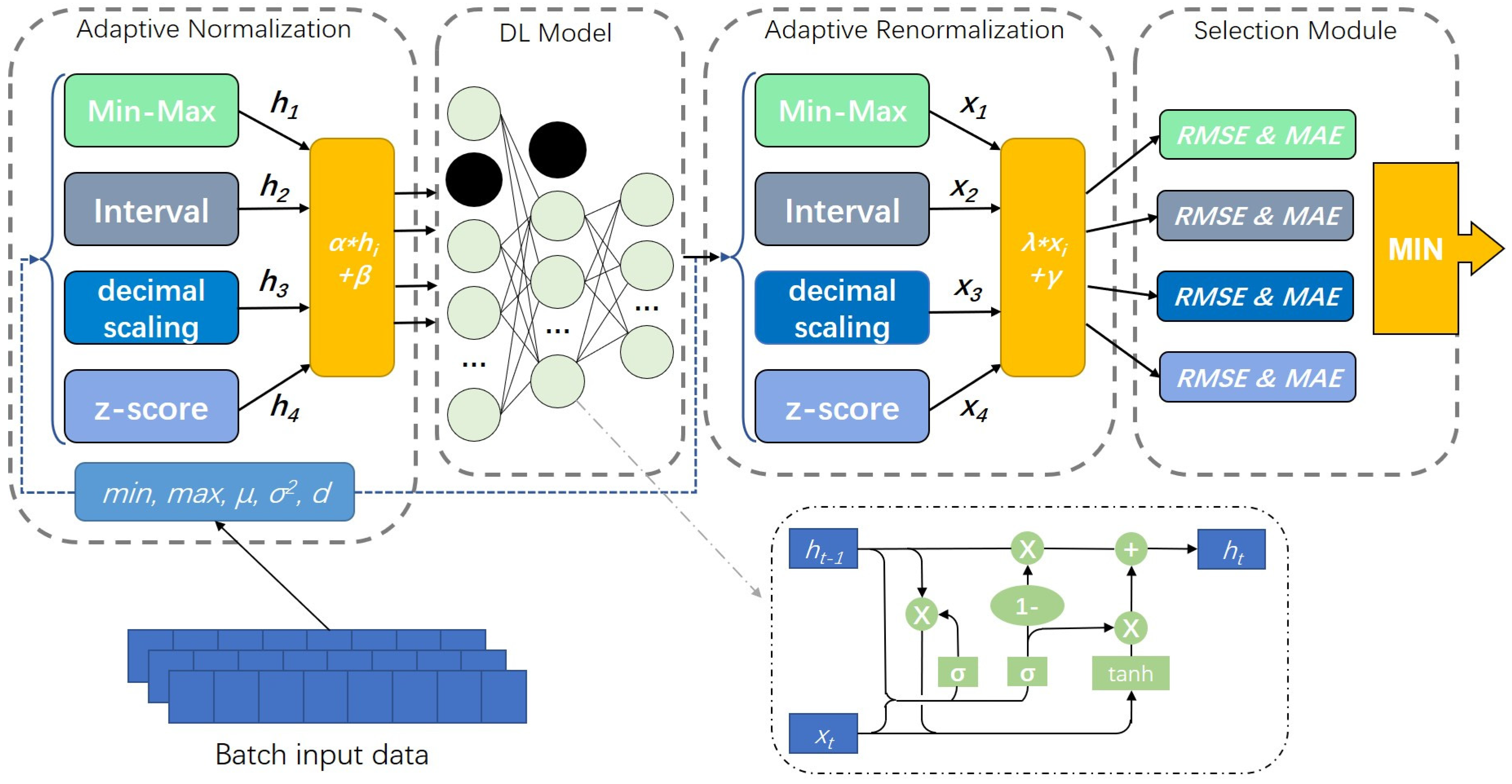
2.1. Networks Structure
2.2. Adaptive Normalization Layer
| Algorithm 1 Normalization Layer Algorithm Framework |
| Input:, , Forgetting weight: m, Selection parameter: mode; Output: // Update max parameters // Update min parameters // Update d parameters if mode = ‘minmax’ then //Min-Max normalization if mode = ‘Interval’ then //Interval normalization if mode = ‘calibrate’ then // Decimal calibration normalization if mode = ‘z-score’ then //z-score normalization if flag = ‘train’ then // Update var parameters else |
2.3. Adaptive Inverse Normalization Layer
| Algorithm 2 Renormalization Layer Algorithm Framework |
| Input:, Output: if mode = ‘minmax’ then //Min-Max renormalization if mode = ‘Interval’ then // Interval renormalization if mode = ‘calibrate’ then // Decimal calibration renormalization if mode = ‘z-score’ then // z-score renormalization if flag = ‘train’ then else |
2.4. Normalization Method Selection Module
3. Experiments and Analysis
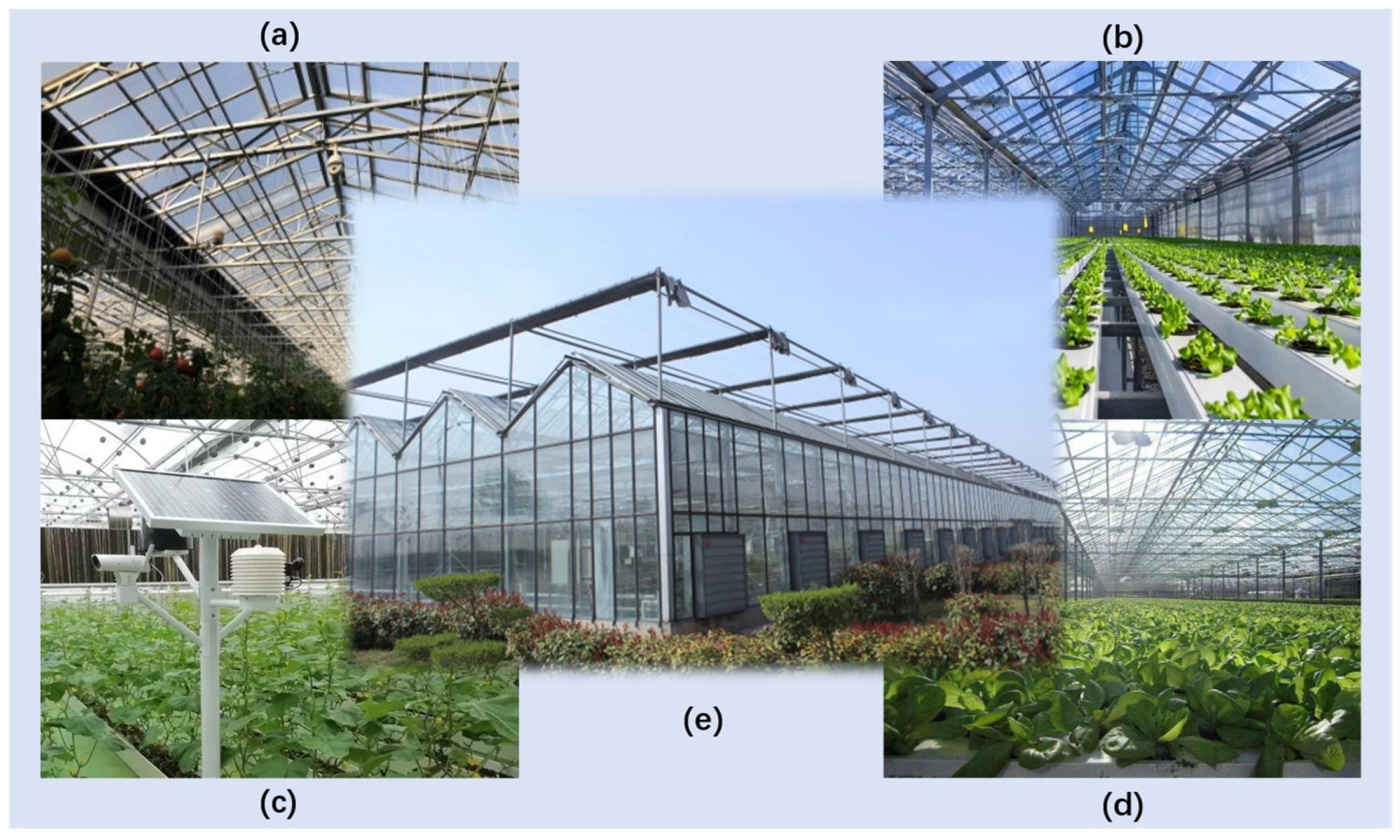
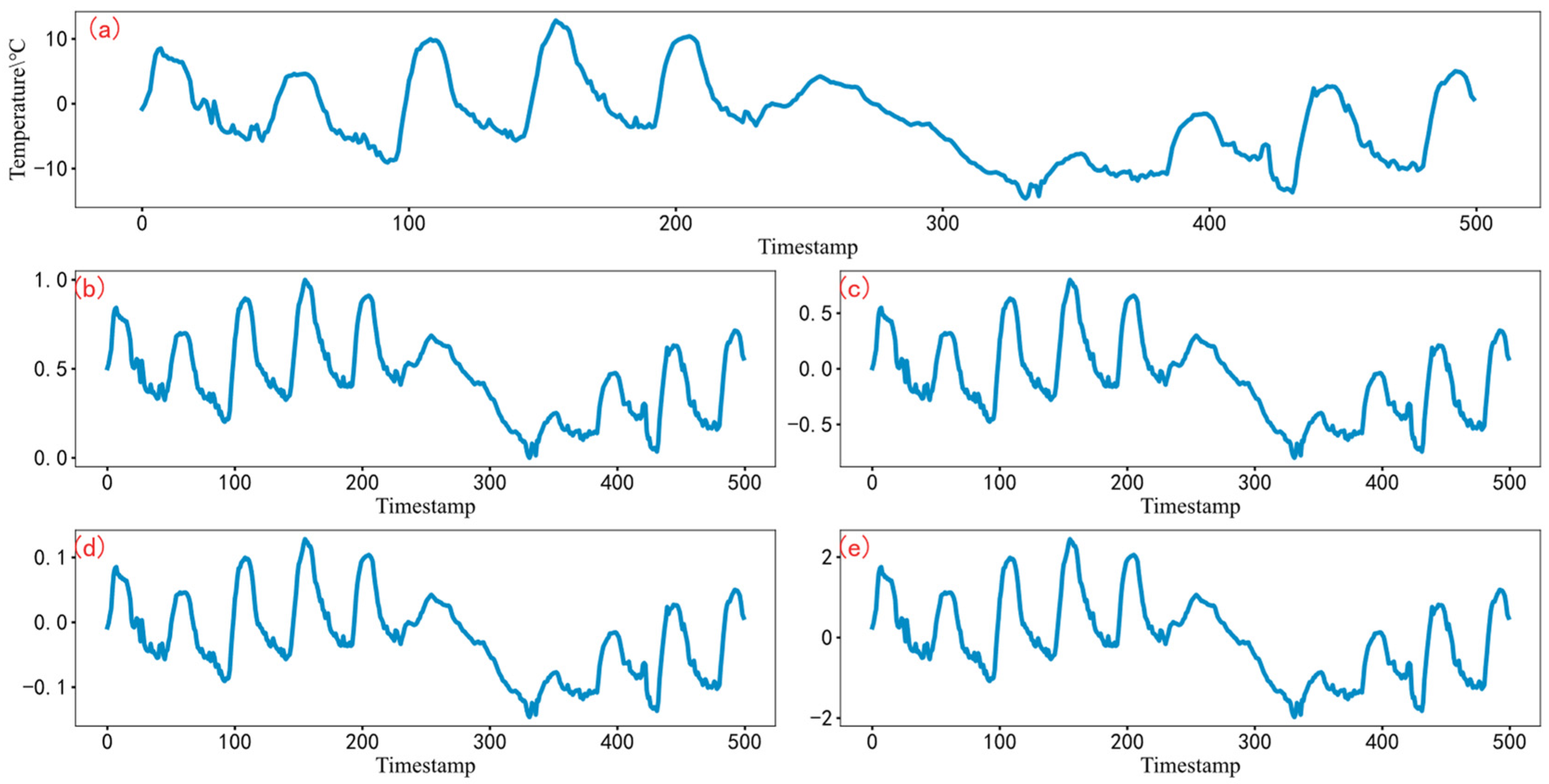
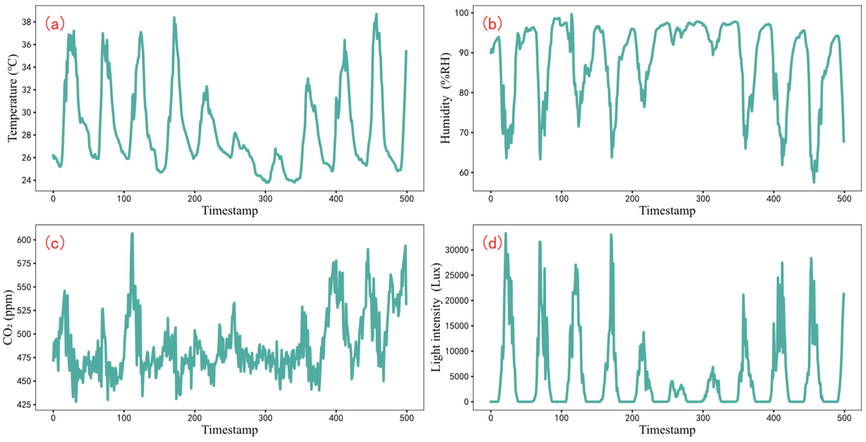
3.1. Experimental Dataset
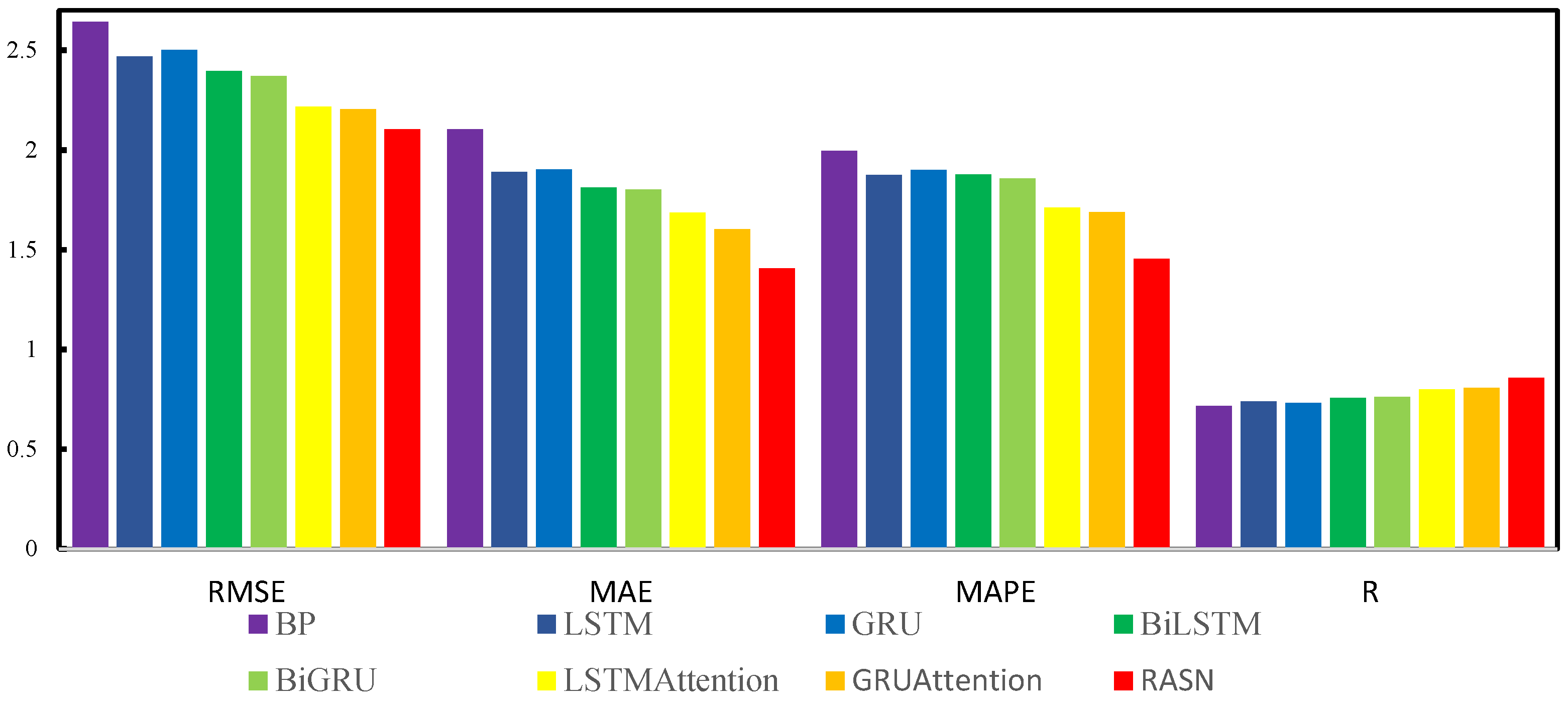
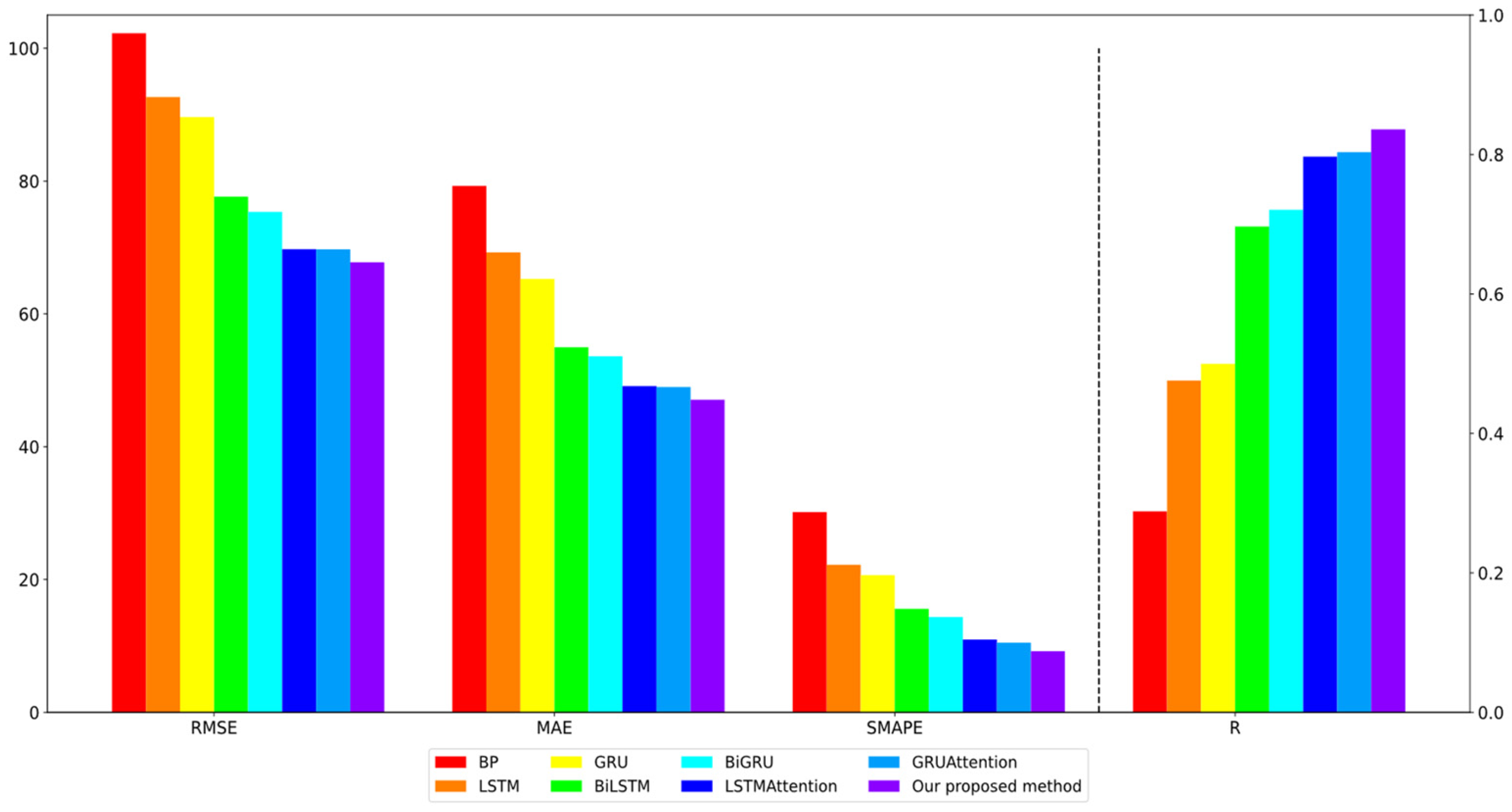
3.2. Evaluation Indexes
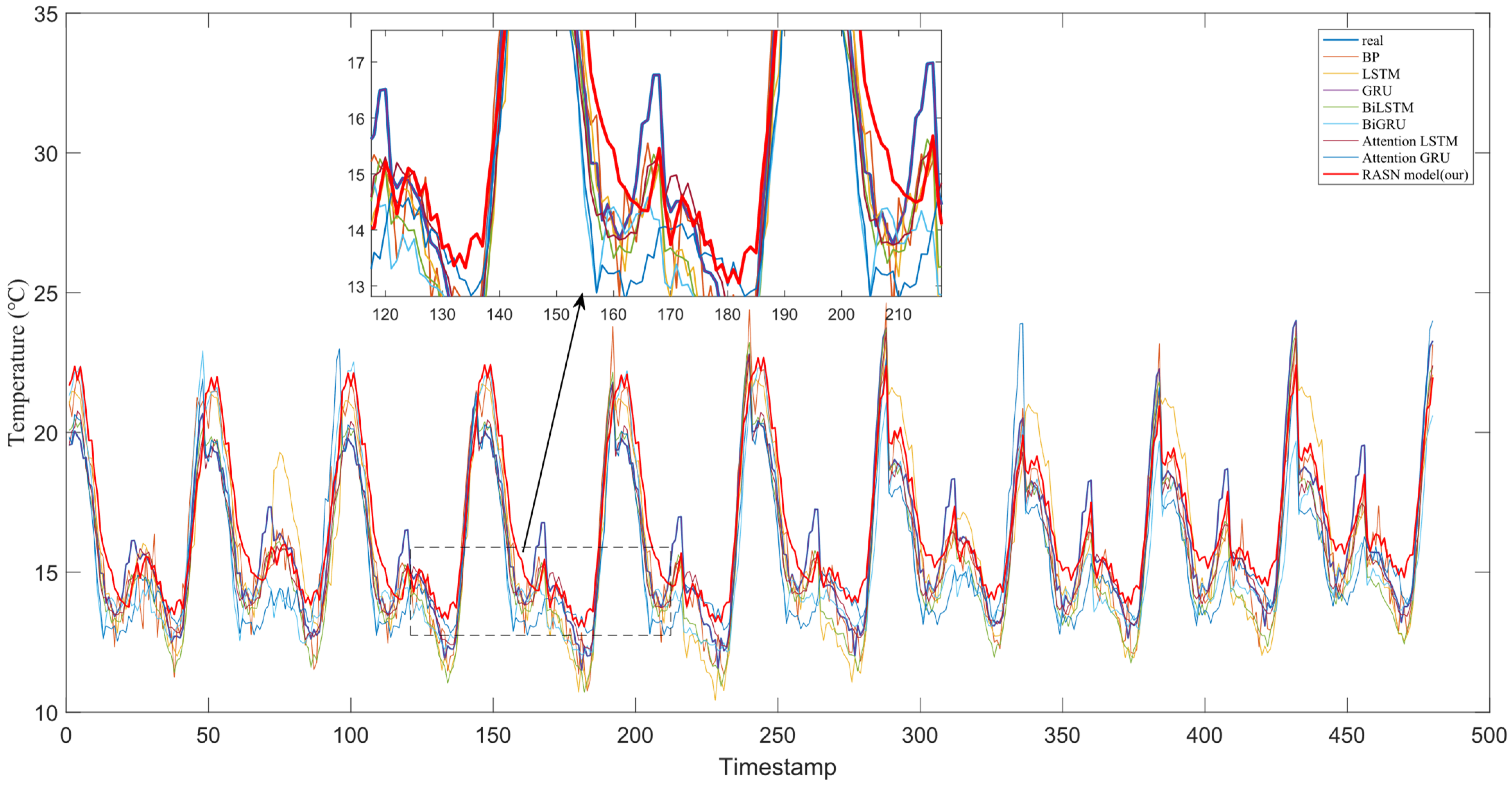
3.3. Prediction in the Greenhouse in Smart Agriculture
4. Conclusions
Author Contributions
Funding
Data Availability Statement
Conflicts of Interest
References
- Zheng, Y.Y.; Kong, J.L.; Jin, X.B.; Wang, X.Y.; Zuo, M. Crop Deep: The crop vision dataset for deep-learning-based classification and detection in precision agriculture. Sensors 2019, 19, 1058. [Google Scholar] [CrossRef] [PubMed] [Green Version]
- Zheng, Y.Y.; Kong, J.L.; Jin, X.B.; Wang, X.Y.; Su, T.L.; Wang, J.L. Probability fusion decision framework of multiple deep neural networks for fine-grained visual classification. IEEE Access 2019, 7, 122740–122757. [Google Scholar] [CrossRef]
- Idrees, S.M.; Alam, M.A.; Agarwal, P. A prediction approach for stock market volatility based on time series data. IEEE Access 2019, 7, 7287–17298. [Google Scholar] [CrossRef]
- Jin, X.B.; Yu, X.H.; Su, T.L.; Yang, D.N.; Bai, Y.T.; Kong, J.L.; Wang, L. Distributed deep fusion predictor for a multi-sensor system based on causality entropy. Entropy 2021, 23, 219. [Google Scholar] [CrossRef]
- Faruk, S.; Yigit, A.; Adnan, K. Hybrid time series forecasting methods for travel time prediction. Phys. A 2021, 579, 126134. [Google Scholar]
- Jin, X.B.; Zheng, W.Z.; Kong, J.L.; Wang, X.Y.; Bai, Y.T.; Su, T.L.; Lin, S. Deep-learning forecasting method for electric power load via attention-based encoder-decoder with bayesian optimization. Energies 2021, 14, 1596. [Google Scholar] [CrossRef]
- Jin, X.B.; Wang, H.X.; Wang, X.Y.; Bai, Y.T.; Su, T.L.; Kong, J.L. Deep-Learning prediction model with serial two-level decomposition based on bayesian optimization. Complexity 2020, 2020, 14. [Google Scholar] [CrossRef]
- Ding, F.; Chen, T. Combined parameter and output estimation of dual-rate systems using an auxiliary model. Automatica 2004, 40, 1739–1748. [Google Scholar] [CrossRef]
- Ding, F.; Chen, T. Parameter estimation of dual-rate stochastic systems by using an output error method. IEEE Trans. Autom. Control 2005, 50, 1436–1441. [Google Scholar] [CrossRef]
- Ding, F.; Shi, Y.; Chen, T. Auxiliary model-based least-squares identification methods for Hammerstein output-error systems. Syst. Control Lett. 2007, 56, 373–380. [Google Scholar] [CrossRef]
- Zhou, Y. Modeling nonlinear processes using the radial basis function-based state-dependent autoregressive models. IEEE Signal Processing Lett. 2020, 27, 1600–1604. [Google Scholar] [CrossRef]
- Zhou, Y.H.; Zhang, X. Partially-coupled nonlinear parameter optimization algorithm for a class of multivariate hybrid models. Appl. Math. Comput. 2022, 414, 126663. [Google Scholar] [CrossRef]
- Zhou, Y.H.; Zhang, X. Hierarchical estimation approach for RBF-AR models with regression weights based on the increasing data length. IEEE Trans. Circuits Syst. II Express Briefs 2021, 68, 3597–3601. [Google Scholar] [CrossRef]
- Ding, F.; Zhang, X.; Xu, L. The innovation algorithms for multivariable state-space models. Int. J. Adapt. Control Signal Processing 2019, 33, 1601–1608. [Google Scholar] [CrossRef]
- Ding, F.; Liu, G.; Liu, X.P. Parameter estimation with scarce measurements. Automatica 2011, 47, 1646–1655. [Google Scholar] [CrossRef]
- Liu, Y.J.; Shi, Y. An efficient hierarchical identification method for general dual-rate sampled-data systems. Automatica 2014, 50, 962–970. [Google Scholar] [CrossRef]
- Zhang, X. Optimal adaptive filtering algorithm by using the fractional-order derivative. IEEE Signal Processing Lett. 2022, 29, 399–403. [Google Scholar] [CrossRef]
- Li, M.H.; Liu, X.M. The filtering-based maximum likelihood iterative estimation algorithms for a special class of nonlinear systems with autoregressive moving average noise using the hierarchical identification principle. Int. J. Adapt. Control Signal Processing 2019, 33, 1189–1211. [Google Scholar] [CrossRef]
- Ding, J.; Liu, X.P.; Liu, G. Hierarchical least squares identification for linear SISO systems with dual-rate sampled-data. IEEE Trans. Autom. Control 2011, 56, 2677–2683. [Google Scholar] [CrossRef]
- Ding, F.; Liu, Y.J.; Bao, B. Gradient-based and least squares based iterative estimation algorithms for multi-input multi-output systems. Proc. Inst. Mech. Eng. Part I J. Syst. Control Eng. 2012, 226, 43–55. [Google Scholar] [CrossRef]
- Xu, L.; Chen, F.Y.; Hayat, T. Hierarchical recursive signal modeling for multi-frequency signals based on discrete measured data. Int. J. Adapt. Control Signal Processing 2021, 35, 676–693. [Google Scholar] [CrossRef]
- Wang, Y.J. Novel data filtering based parameter identification for multiple-input multiple-output systems using the auxiliary model. Automatica 2016, 71, 308–313. [Google Scholar] [CrossRef]
- Jin, X.B.; Yu, X.H.; Wang, X.Y.; Bai, Y.T.; Su, T.L.; Kong, J.L. Deep learning predictor for sustainable precision agriculture based on internet of things system. Sustainability 2020, 12, 1433. [Google Scholar] [CrossRef] [Green Version]
- Jin, X.B.; Yang, N.X.; Wang, X.Y.; Bai, Y.T.; Su, T.L.; Kong, J.L. Deep hybrid model based on EMD with classification by frequency characteristics for long-term air quality prediction. Mathematics 2020, 8, 214. [Google Scholar] [CrossRef] [Green Version]
- Zhen, T.; Kong, J.; Yan, L. Hybrid Deep-Learning framework based on gaussian fusion of multiple spatiotemporal networks for walking gait phase recognition. Complexity 2020, 2020, 1–17. [Google Scholar] [CrossRef]
- Jin, X.B.; Zheng, W.Z.; Kong, J.L.; Wang, X.Y.; Zuo, M.; Zhang, Q.C.; Lin, S. Deep-Learning temporal predictor via bi-directional self-attentive Encoder-Decoder framework for IoT-based environmental sensing in intelligent greenhouse. Agriculture 2021, 11, 802. [Google Scholar] [CrossRef]
- Jin, X.B.; Yang, N.X.; Wang, X.Y.; Bai, Y.T.; Su, T.L.; Kong, J.L. Integrated predictor based on decomposition mechanism for PM2.5 long-term prediction. Appl. Sci. 2019, 9, 4533. [Google Scholar] [CrossRef] [Green Version]
- Kim, H.J.; Baek, J.W.; Chung, K. Associative knowledge graph using fuzzy clustering and Min-Max normalization in video contents. IEEE Access 2021, 9, 74802–74816. [Google Scholar] [CrossRef]
- Jain, A.; Nandakumar, K.; Ross, A. Score normalization in multimodal biometric systems. Pattern Recognit. 2013, 38, 2270–2285. [Google Scholar] [CrossRef]
- Summers, C.; Dinneen, M.J. Four things everyone should know to improve Batch Normalization. ICLR 2020, 1–18. [Google Scholar]
- Pan, H.; Niu, X.; Li, R.; Dou, Y.; Jiang, H. Annealed gradient descent for Deep Learning. Neurocomputing 2019, 380, 201–211. [Google Scholar] [CrossRef]
- Zou, Z.X.; Yang, Y.M.; Fan, Z.Q.; Tang, H.M.; Zou, M.; Hu, X.L.; Xiong, C.R.; Ma, J.W. Suitability of data preprocessing methods for landslide displacement forecasting. Stoch. Environ. Res. Risk Assess. 2020, 34, 1105–1119. [Google Scholar] [CrossRef]
- Singh, D.; Singh, B. Feature wise normalization: An effective way of normalizing data. Pattern Recognit. 2022, 122, 108307. [Google Scholar] [CrossRef]
- Jain, S.; Shukla, S.; Wadhvani, R. Dynamic selection of normalization techniques using data complexity measures. Expert Syst. Appl. 2018, 106, 252–262. [Google Scholar] [CrossRef]
- Ioffe, S.; Szegedy, C. Batch Normalization: Accelerating deep network training by reducing internal covariate shift. arXiv 2015, arXiv:1502.03167. [Google Scholar]
- Passalis, N.; Tefas, A.; Kanniainen, J.; Gabbouj, M.; Iosifidis, A. Deep adaptive input normalization for time series forecasting. IEEE Trans. Neural Netw. Learn. Syst. 2019, 99, 1–6. [Google Scholar] [CrossRef] [PubMed] [Green Version]
- Tomar, D.; Lortkipanidze, M.; Vray, G.; Bozorgtabar, B.; Thiran, J.P. Self-Attentive spatial adaptive normalization for cross-modality domain adaptation. IEEE Trans. Med. Imaging 2021, 40, 2926–2938. [Google Scholar] [CrossRef] [PubMed]
- Park, T.; Liu, M.Y.; Wang, T.C.; Zhu, J.Y. Semantic image synthesis with spatially-adaptive normalization. In Proceedings of the IEEE/CVF Conference on Computer Vision and Pattern Recognition (CVPR), Long Beach, CA, USA, 15–20 June 2019; 2019; pp. 1–10. [Google Scholar]
- Yan, J.J.; Wan, R.S.; Zhang, X.Y.; Zhang, W.; Wei, Y.C.; Sun, J. Towards stabilizing batch statistics in backward propagation of Batch Normalization. arXiv 2020, arXiv:2001.06838. [Google Scholar]
- Du, Y.J.; Zhen, X.T.; Shao, L.; Snoek, C.G.M. MetaNorm: Learning to normalize few-shot batches across domains. In Proceedings of the International Conference on Learning Representations, online, 3–7 May 2021; pp. 1–23. [Google Scholar]
- Luo, P.; Ren, J.M.; Peng, Z.L.; Zhang, R.M.; Li, J.Y. Differentiable learning-to-normalize via switchable normalization. arXiv 2019, arXiv:1806.10779. [Google Scholar]
- Shao, W.Q.; Meng, T.J.; Li, J.Y.; Zhang, R.M.; Wang, X.G.; Luo, P. SSN: Learning sparse switchable normalization via SparsestMax. Int. J. Comput. Vis. 2020, 128, 2107–2125. [Google Scholar] [CrossRef] [Green Version]
- Yang, S.; Yu, S.; Zhao, B.; Wang, Y. Reducing the feature divergence of RGB and near-infrared images using Switchable Normalization. In Proceedings of the IEEE/CVF Conference on Computer Vision and Pattern Recognition (CVPR) Workshops, Seattle, WA, USA, 13–19 June 2020; pp. 206–211. [Google Scholar]
- Giraldo, L.G.S.; Schwartz, O. Integrating flexible normalization into midlevel representations of deep convolutional neural Networks. Neural Comput. 2019, 31, 2138–2176. [Google Scholar] [CrossRef] [PubMed] [Green Version]
- Bermudez-Edo, M.; Barnaghi, P.; Moessner, K. Analysing real world data streams with spatio-temporal correlations: Entropy vs. Pearson correlation. Autom. Constr. 2018, 88, 87–100. [Google Scholar] [CrossRef]
- Wang, W.; Li, W. Research on trend analysis method of multi-series economic data based on correlation enhancement of deep learning. Neural Comput. Appl. 2021, 33, 4815–4831. [Google Scholar] [CrossRef]
- Khodabandelou, G.; Jung, P.G.; Amirat, Y.; Mohammed, S. Attention-Based gated recurrent unit for gesture recognition. IEEE Trans. Autom. 2020, 18, 495–507. [Google Scholar] [CrossRef]
- Tian, L.; Li, X.; Ye, Y.; Xie, P.; Li, Y. A generative adversarial gated recurrent unit model for precipitation nowcasting. IEEE Geosci. Remote Sens. Lett. 2020, 17, 601–605. [Google Scholar] [CrossRef]
- Shen, X.; Tian, X.; Liu, T.; Xu, F.; Tao, D.C. Continuous dropout. IEEE Trans. Neural Netw. Learn. Syst. 2018, 29, 3926–3937. [Google Scholar] [CrossRef] [PubMed]
- Yu, J.; Kim, S.B.; Bai, J.; Han, S.W. Comparative study on exponentially weighted moving average approaches for the self-starting forecasting. Appl. Sci. 2020, 10, 7351. [Google Scholar] [CrossRef]
- Kong, J.L.; Wang, H.X.; Jin, X.B.; Wang, X.Y.; Fang, X.; Lin, S. Multi-stream hybrid architecture based on cross-level fusion strategy for fine-grained crop species recognition in precision agriculture. Comput. Electron. Agric. 2021, 185, 106134. [Google Scholar] [CrossRef]
- Idoje, G.; Dagiuklas, T.; Iqbal, M. Survey for smart farming technologies: Challenges and issues. Comput. Electr. Eng. 2021, 92, 107104. [Google Scholar] [CrossRef]
- Kong, J.L.; Yang, C.C.; Wang, J.L.; Zuo, M.; Jin, X.B.; Lin, S. Deep-stacking network approach by multisource data mining for hazardous risk identification in IoT-based intelligent food management systems. Comput. Intell. Neurosci. 2021, 2021, 1194565. [Google Scholar] [CrossRef] [PubMed]
- Chakrabarty, A.; Mansoor, N.; Uddin, M.I.; Al-adaileh, M.H.; Alsharif, N.; Alsaade, F.W. Prediction approaches for Smart cultivation: A comparative study. Complexity 2021, 2021, 1–16. [Google Scholar] [CrossRef]
- Yang, S.T.; Luo, L.N.; Tan, B.H. Research on sports performance prediction based on BP neural network. Mob. Inf. Syst. 2021, 2021, 8. [Google Scholar] [CrossRef]
- Van Houdt, G.; Mosquera, C.; Nápoles, G. A review on the long short-term memory model. Artif. Intell. Rev. 2020, 53, 5929–5955. [Google Scholar] [CrossRef]
- Jin, X.B.; Gong, W.T.; Kong, J.L.; Bai, Y.T.; Su, T.L. Variational Bayesian deep network with data self-screening layer for massive time-series data forecasting. Entropy 2022, 24, 335. [Google Scholar] [CrossRef]
- Petroanu, D.M.; Prjan, A. Electricity consumption forecasting based on a bidirectional long-short-term memory artificial neural network. Sustainability 2020, 13, 104. [Google Scholar] [CrossRef]
- Meng, F.; Song, T.; Xu, D.Y.; Xie, P.F.; Li, Y. Forecasting tropical cyclones wave height using bidirectional gated recurrent unit. Ocean Eng. 2021, 234, 108795. [Google Scholar] [CrossRef]
- Niu, Z.; Yu, Z.; Tang, W.; Wu, Q.; Reformat, M. Wind power forecasting using attention-based gated recurrent unit network. Energy 2020, 196, 117081. [Google Scholar] [CrossRef]
- Ding, F.; Lv, L.; Pan, J.; Wang, X.K.; Jin, X.B. Two-stage gradient-based iterative estimation methods for controlled autoregressive systems using the measurement data. Int. J. Control Autom. Syst. 2020, 18, 886–896. [Google Scholar] [CrossRef]
- Ding, F.; Wang, F.F.; Wu, M.H. Decomposition based least squares iterative identification algorithm for multivariate pseudo-linear ARMA systems using the data filtering. J. Frankl. Inst. 2017, 354, 1321–1339. [Google Scholar] [CrossRef]
- Zhang, X. Hierarchical parameter and state estimation for bilinear systems. Int. J. Syst. Sci. 2020, 51, 275–290. [Google Scholar] [CrossRef]
- Xu, L.; Zhu, Q.M. Decomposition strategy-based hierarchical least mean square algorithm for control systems from the impulse responses. Int. J. Syst. Sci. 2021, 52, 1806–1821. [Google Scholar] [CrossRef]
- Zhang, X.; Xu, L.; Hayat, T. Combined state and parameter estimation for a bilinear state space system with moving average noise. J. Frankl. Inst. 2018, 355, 3079–3103. [Google Scholar] [CrossRef]
- Pan, J.; Jiang, X.; Ding, W. A filtering based multi-innovation extended stochastic gradient algorithm for multivariable control systems. Int. J. Control Autom. Syst. 2017, 15, 1189–1197. [Google Scholar] [CrossRef]
- Zhang, X.; Yang, E.F. State estimation for bilinear systems through minimizing the covariance matrix of the state estimation errors. Int. J. Adapt Control Signal Processing 2019, 33, 1157–1173. [Google Scholar] [CrossRef]
- Pan, J.; Ma, H.; Liu, Q.Y. Recursive coupled projection algorithms for multivariable output-error-like systems with coloured noises. IET Signal Processing 2020, 14, 455–466. [Google Scholar] [CrossRef]
- Ding, F.; Liu, G.; Liu, X.P. Partially coupled stochastic gradient identification methods for non-uniformly sampled systems. IEEE Trans. Autom. Control 2010, 55, 1976–1981. [Google Scholar] [CrossRef]
- Ding, F.; Shi, Y.; Chen, T. Performance analysis of estimation algorithms of non-stationary ARMA processes. IEEE Trans. Signal Processing 2006, 54, 1041–1053. [Google Scholar] [CrossRef]
- Wang, Y.J.; Wu, M.H. Recursive parameter estimation algorithm for multivariate output-error systems. J. Frankl. Inst. 2018, 355, 5163–5181. [Google Scholar] [CrossRef]
- Xu, L. Separable multi-innovation Newton iterative modeling algorithm for multi-frequency signals based on the sliding measurement window. Circuits Syst. Signal Processing 2022, 41, 805–830. [Google Scholar] [CrossRef]
- Xu, L. Separable Newton recursive estimation method through system responses based on dynamically discrete measurements with increasing data length. Int. J. Control Autom. Syst. 2022, 20, 432–443. [Google Scholar] [CrossRef]
- Xu, L.; Yang, E.F. Auxiliary model multiinnovation stochastic gradient parameter estimation methods for nonlinear sandwich systems. Int. J. Robust Nonlinear Control 2021, 31, 148–165. [Google Scholar] [CrossRef]
- Zhang, X. Adaptive parameter estimation for a general dynamical system with unknown states. Int. J. Robust Nonlinear Control 2020, 30, 1351–1372. [Google Scholar] [CrossRef]
- Zhang, X. Recursive parameter estimation methods and convergence analysis for a special class of nonlinear systems. Int. J. Robust Nonlinear Control 2020, 30, 1373–1393. [Google Scholar] [CrossRef]
- Zhang, X. Recursive parameter estimation and its convergence for bilinear systems. IET Control Theory Appl. 2020, 14, 677–688. [Google Scholar] [CrossRef]
- Liu, S.Y.; Hayat, T. Hierarchical principle-based iterative parameter estimation algorithm for dual-frequency signals. Circuits Syst. Signal Processing 2019, 38, 3251–3268. [Google Scholar] [CrossRef]
- Wan, L.J. Decomposition- and gradient-based iterative identification algorithms for multivariable systems using the multi-innovation theory. Circuits Syst. Signal Processing 2019, 38, 2971–2991. [Google Scholar] [CrossRef]
- Jin, X.B.; Yang, N.X.; Wang, X.Y.; Bai, Y.T. Hybrid deep learning predictor for smart agriculture sensing based on empirical mode decomposition and gated recurrent unit group model. Sensors 2020, 20, 1334. [Google Scholar] [CrossRef] [Green Version]
- Wang, X.H. Modified particle filtering-based robust estimation for a networked control system corrupted by impulsive noise. Int. J. Robust Nonlinear Control 2022, 32, 830–850. [Google Scholar] [CrossRef]
- Pan, J.; Li, W.; Zhang, H.P. Control algorithms of magnetic suspension systems based on the improved double exponential reaching law of sliding mode control. Int. J. Control Autom. Syst. 2018, 16, 2878–2887. [Google Scholar] [CrossRef]
- Ma, H.; Pan, J.; Ding, W. Partially-coupled least squares based iterative parameter estimation for multi-variable output-error-like autoregressive moving average systems. IET Control Theory Appl. 2019, 13, 3040–3051. [Google Scholar] [CrossRef]
- Ding, F.; Liu, X.P.; Yang, H.Z. Parameter identification and intersample output estimation for dual-rate systems. IEEE Trans. Syst Man Cybern. Part A Syst. Hum. 2008, 38, 966–975. [Google Scholar] [CrossRef]
- Ding, F.; Liu, X.P.; Liu, G. Multiinnovation least squares identification for linear and pseudo-linear regression models. IEEE Trans. Syst. Man Cybern. Part B Cybern. 2010, 40, 767–778. [Google Scholar] [CrossRef]
- Xu, L.; Song, G.L. A recursive parameter estimation algorithm for modeling signals with multi-frequencies. Circuits Syst. Signal Processing 2020, 39, 4198–4224. [Google Scholar] [CrossRef]
- Jin, X.B.; Gong, W.T.; Kong, J.L.; Bai, Y.T.; Su, T.L. PFVAE: A planar flow-based variational auto-encoder prediction model for time-series data. Mathematics 2022, 10, 610. [Google Scholar] [CrossRef]
- Xu, L.; Sheng, J. Separable multi-innovation stochastic gradient estimation algorithm for the nonlinear dynamic responses of systems. Int. J. Adapt. Control Signal Processing 2020, 34, 937–954. [Google Scholar] [CrossRef]
- Hou, J.; Chen, F.W.; Li, P.H.; Zhu, Z.Q. Gray-box parsimonious subspace identification of Hammerstein-type systems. IEEE Trans. Ind. Electron. 2021, 68, 9941–9951. [Google Scholar] [CrossRef]
- Zhao, Z.Y.; Zhou, Y.Q.; Wang, X.Y.; Wang, Z.Y.; Bai, Y.T. Water quality evolution mechanism modeling and health risk assessment based on stochastic hybrid dynamic systems. Expert Syst. Appl. 2022, 193, 116404. [Google Scholar] [CrossRef]
- Chen, Q.; Zhao, Z.Y.; Wang, X.Y.; Xiong, K. Microbiological predictive modeling and risk analysis based on the one-step kinetic integrated Wiener process. Innovat. Food Sci. Emerg. Technol. 2022, 75, 102912. [Google Scholar] [CrossRef]
- Shu, J.; He, J.C.; Li, L. MSIS: Multispectral instance segmentation method for power equipment. Comput. Intell. Neurosci. 2022, 2022, 2864717. [Google Scholar] [CrossRef]
- Peng, H.X.; He, W.J.; Zhang, Y.L.; Li, X.W.; Ding, Y.; Menon, V.G.; Verma, S. Covert non-orthogonal multiple access communication assisted by multi-antenna jamming. Phys. Comm. 2022, 2022, 101598. [Google Scholar] [CrossRef]


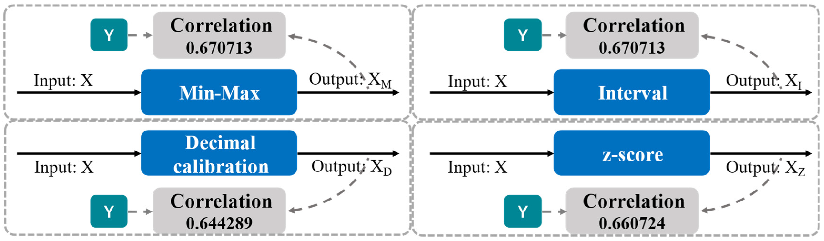
| Methods | Between X and Y | Between XM and Y (Min-Max Normalization) | Between XI and Y (Interval Normalization) | Between XD and Y (Decimal Calibration) | Between XZ and Y (z-Score Normalization) |
|---|---|---|---|---|---|
| Correlation | 0.660778 | 0.670713 | 0.670713 | 0.644289 | 0.660724 |
| MODELS | RMSE | MAE | MSE | MAPE | R |
|---|---|---|---|---|---|
| BP [55] | 2.2326 | 1.6305 | 4.9848 | 1.0068 | 0.8358 |
| LSTM [56] | 2.3901 | 1.8321 | 5.7132 | 1.0049 | 0.8034 |
| GRU [57] | 2.4916 | 1.8748 | 5.7296 | 1.0034 | 0.7814 |
| BiLSTM [58] | 2.3745 | 1.8002 | 5.6022 | 0.9991 | 0.8124 |
| BiGRU [59] | 2.3603 | 1.7999 | 5.5714 | 0.9873 | 0.8207 |
| Attention_LSTM [6] | 2.2372 | 1.7033 | 5.3406 | 1.0112 | 0.8341 |
| Attention_GRU [60] | 2.1542 | 1.6613 | 4.6404 | 1.0008 | 0.8426 |
| RASN (our) | 1.9032 | 1.4609 | 3.4609 | 0.7001 | 0.8928 |
| MODELS | RMSE | MAE | MSE | MAPE | R |
|---|---|---|---|---|---|
| BP [55] | 2.6413 | 2.1036 | 6.7658 | 1.9965 | 0.7161 |
| LSTM [56] | 2.4681 | 1.8895 | 6.2634 | 1.8759 | 0.7379 |
| GRU [57] | 2.5015 | 1.9033 | 6.3631 | 1.8996 | 0.7321 |
| BiLSTM [58] | 2.3946 | 1.8112 | 6.0986 | 1.8769 | 0.7568 |
| BiGRU [59] | 2.3711 | 1.8012 | 6.0124 | 1.8586 | 0.7621 |
| Attention_LSTM [6] | 2.2172 | 1.6863 | 5.8735 | 1.7121 | 0.7989 |
| Attention_GRU [60] | 2.2025 | 1.6036 | 5.8632 | 1.6876 | 0.8068 |
| RASN (our) | 2.1017 | 1.4077 | 5.6007 | 1.4553 | 0.8572 |
| MODELS | RMSE | MAE | MAPE | R |
|---|---|---|---|---|
| BP [55] | 102.2564 | 79.2658 | 30.1542 | 0.3026 |
| LSTM [56] | 92.6584 | 69.2546 | 22.2165 | 0.4996 |
| GRU [57] | 89.6359 | 65.2597 | 20.6541 | 0.5248 |
| BiLSTM [58] | 77.6521 | 54.9854 | 15.5896 | 0.7316 |
| BiGRU [59] | 75.3654 | 53.6218 | 14.3584 | 0.7568 |
| Attention_LSTM [6] | 69.7441 | 49.1254 | 10.9651 | 0.8368 |
| Attention_GRU [60] | 69.7258 | 48.9856 | 10.4852 | 0.8436 |
| RASN (our) | 67.7661 | 47.0659 | 9.2122 | 0.8778 |
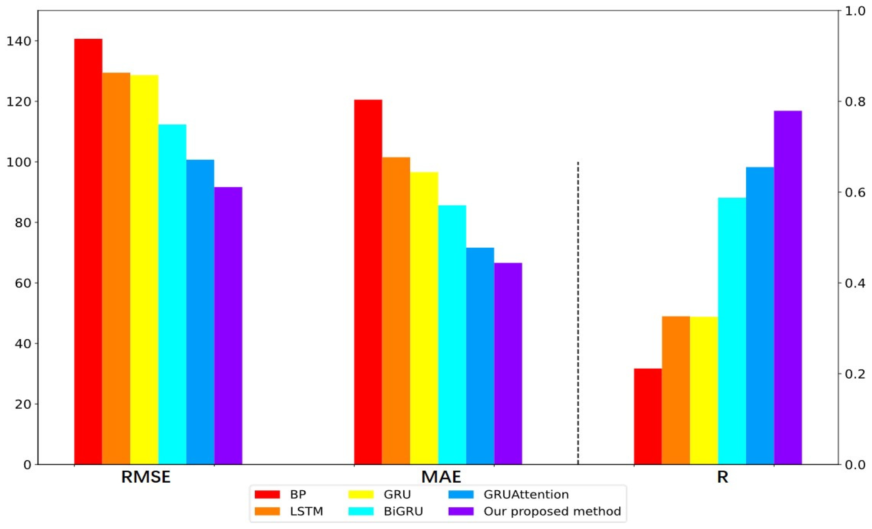
| MODELS | RMSE | MAE | R |
|---|---|---|---|
| BP [55] | 140.6614 | 120.5418 | 0.2114 |
| LSTM [56] | 129.4581 | 101.5268 | 0.3265 |
| GRU [57] | 128.6524 | 96.5924 | 0.3254 |
| BiGRU [59] | 112.3584 | 85.6521 | 0.5876 |
| Attention_GRU [60] | 100.7216 | 71.6594 | 0.6551 |
| RASN (our) | 91.6691 | 66.6154 | 0.7791 |
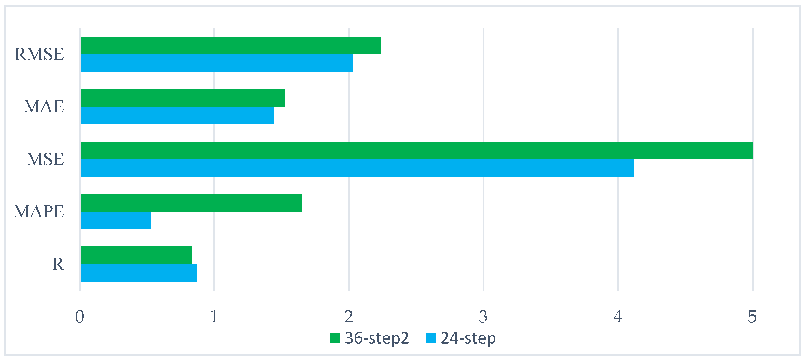
| STEP | RMSE | MAE | MSE | MAPE | R |
|---|---|---|---|---|---|
| 36-step | 2.2364 | 1.5242 | 5.0014 | 1.6478 | 0.8358 |
| 24-step | 2.0289 | 1.4467 | 4.1165 | 0.5279 | 0.8673 |
Publisher’s Note: MDPI stays neutral with regard to jurisdictional claims in published maps and institutional affiliations. |
© 2022 by the authors. Licensee MDPI, Basel, Switzerland. This article is an open access article distributed under the terms and conditions of the Creative Commons Attribution (CC BY) license (https://creativecommons.org/licenses/by/4.0/).
Share and Cite
Jin, X.; Zhang, J.; Kong, J.; Su, T.; Bai, Y. A Reversible Automatic Selection Normalization (RASN) Deep Network for Predicting in the Smart Agriculture System. Agronomy 2022, 12, 591. https://doi.org/10.3390/agronomy12030591
Jin X, Zhang J, Kong J, Su T, Bai Y. A Reversible Automatic Selection Normalization (RASN) Deep Network for Predicting in the Smart Agriculture System. Agronomy. 2022; 12(3):591. https://doi.org/10.3390/agronomy12030591
Chicago/Turabian StyleJin, Xuebo, Jiashuai Zhang, Jianlei Kong, Tingli Su, and Yuting Bai. 2022. "A Reversible Automatic Selection Normalization (RASN) Deep Network for Predicting in the Smart Agriculture System" Agronomy 12, no. 3: 591. https://doi.org/10.3390/agronomy12030591