Analysis of Turbulent Air Flow Characteristics Due to the Presence of a 13 × 30 Threads·cm⁻² Insect Proof Screen on the Side Windows of a Mediterranean Greenhouse

Abstract

Insect-proof screens are a frequent passive method to restrict the entrance of insects into greenhouses. However, the installation of these screens also has a negative effect on natural ventilation, which is reflected in the turbulence and velocity of the airflow inside the greenhouse. The turbulent characteristics of airflow through an insect-proof screen installed in the greenhouse windows have not been studied thoroughly in the literature. The present work focuses on the use of two simultaneous 3D sonic anemometers to study the impact of the use of a 13 × 30 threads·cm⁻² insect-proof screen on the turbulence properties of the micro and microscale airflow turbulence. Four tests have been carried out in windward-oriented side windows of a Mediterranean greenhouse. Results demonstrate that the approach of using two simultaneous 3D sonic anemometers for the first time allows one to observe that the effect is different for the three components of the velocity vector field, and there is a strong connection between the simultaneous conditions inside and outside of the greenhouse. Useful information and data on the effect of using a 13 × 30 threads·cm⁻² insect-proof screen are also provided. To give details on the impact of screens in the turbulent properties of ventilation is essential for any commercial distribution, as well as providing important data in the design and development of more efficient insect-proof screens.

1. Introduction

Currently, natural ventilation systems in greenhouses are conditioned by the widespread use of insect-proof screens with high thread density and low porosity. The use of these screens pursues the objective of reducing the entry of insects that are harmful to crops. Its use is essential in Mediterranean regions, as well as tropical-subtropical countries, where climatic conditions favor the spread of insect pests, thus representing an important issue in agriculture. The installation of insect-proof screens (IPS) represents a passive, low-cost protection mechanism against migratory insects, dramatically reducing the damage to crops and insect-vectored diseases [1,2]. The use of IPS, in essence, exhibits multifold objectives, one of which is to reduce the need to use pesticides [2,3,4,5]. This satisfies international sustainability regulations and attracts certifications on biological control. It also prevents scaping beneficial insect pollinators [2]. As a reference on the impact on the greenhouse economy, Taylor et al. [5] estimated that the losses caused by the Bemisia tabaci (also known as a sweetpotato whitefly) were up to between 15 and 32 million dollars during 1980 and 1990. These significant economic losses could have been easily avoided with the use of efficient IPS.

IPS are designed to reduce the entry of insects into the greenhouse. It is obvious that the size of the pores needs to be smaller than the size of the smallest damaging insect to be deterred. The main harmful insects in the Mediterranean region are aphids (Myzus persicae Sulzev and Aphis gossipii Glover), the leaf miner (Liriomyza sp.), the whitefly (Trialeurodes vaporariorum Westwood and Bemisia tabaci Gennadius), and especially thrips (Frankliniella occidentalis Pergande and Thrips tabaci Lindeman), and the tomato moth (Tuta absolu Meyrick), which recently appeared in the province of Almería (Spain). The most difficult insects to prevent from entering the greenhouse are thrips, due to two reasons: (i) because of their small size, mean width of the thorax between 184.4 µm for males and 245.5 µm for females [6], and (ii) because of their intelligence and ability to overcome the physical barrier created by the interlaced mesh by crawling across the IPS pores, the thrips are very thin from a lateral point of view and can use the whole length to pass through the screens [3].

The main drawback of the use of IPS is the reduction of the air renewal capacity of natural ventilation systems and its consequent inefficient microclimate conditions inside the greenhouse. For greenhouses without IPS, the recommended values of the ventilation surface to keep adequate microclimatic conditions were estimated around 30% [7], between 18 and 25% [8], 15% [9], or between 15 and 25% [10]. With the incorporation of IPSs in greenhouses, average ventilation has been decreased, being very difficult to achieve high-performance microclimate conditions while preventing the entrance of insects into crops [11]. The effect on ventilation by the installation of IPSs can lead to misaligning the heat and mass exchange with the exterior, leading to unpunctual growth of crops and development and spread of fungal diseases [1,12,13,14]. The effect of installing IPS on natural ventilation and the microclimate of greenhouses has been studied by many authors before. Yang et al. [15] observed significant reductions in ventilation and significant increases in indoor temperature values. Similarly, Teitel et al. [16] identified that the presence of the IPS has an important impact on the levels of turbulence inside the greenhouse. Bartzanas et al. [17] observed that an IPS of 53% of porosity affects ventilation rate up to 50% and increases indoor temperature by 4 °C. Fatnassi et al. [18,19,20] also noticed that air humidity is strongly affected by the installation of IPS. The researchers concluded that humidity and temperature inside and outside the greenhouse could be doubled (with an IPS of 41% of porosity) or tripled (with IPS of 20% of porosity). Harmanto et al. [14] studied, by means of an energy and mass balance, the effect on ventilation of three IPS (with porosities of 41, 38, and 30%). Compared to the most porous IPS, the less porous screen reduced 50% of the ventilation rate capacity while increasing the indoor temperature by 3 °C. The IPS with intermediate porosity reduced 35% of the ventilation rate while increasing the indoor temperature by 1 °C. Baeza et al. [21] also concluded that an IPS with a 28% of porosity could lead to a reduction of the ventilation rate—depending on the size of the greenhouse—by as much as 77–87%.

The reduction in the greenhouse ventilation rate due to IPSs can be considered proportional to the reduction in the speed of air passage through the windows [22] because of the reduction in the discharge coefficient [2]. López-Martínez et al. [23] used sonic anemometry to determine airflow patterns in a multi-tunnel greenhouse, where it was suggested the installation of ailerons to guide the flow being impinged more or less perpendicularly to the IPS. Lately, López-Martínez et al. [24] studied the installation of three different IPSs to observe the impact on the difference between temperature and air velocity inside and outside Mediterranean greenhouses, as well as the discharge coefficient, and to find relevant relations with geometric characteristics of the mesh.

In order to increase the effectiveness of the IPSs as a physical barrier, it is necessary to reduce the size of the pore, which is generally associated with a reduction in porosity (which reduces the ventilation rate and increases the temperature and humidity inside the greenhouse [18,19]). The study of the aerodynamic properties of IPS is then also an important aspect in order to understand their impact on ventilation. López-Martínez et al. [25] obtained mathematical models for the characterization of insect-proof screens, which were related to geometric aspects (diameter of threads, porosity, etc.) with parameters of interest for ventilation, such as permeability, inertia factor, and pressure drop coefficient. To overcome the ambiguity of the characterization of porosity as a 2D measure, which does not take into account the thickness of screens, Granados-Ortiz et al. [26] developed a mathematical approach to characterize a three-dimensional porosity (volumetric porosity) as a more complete and accurate estimation.

In some studies, the reduction in the ventilation rate due to the use of IPSs has been quantified between 77–87% for a mesh with a porosity of 28% [21] and by 50% for a mesh with a porosity of 53% [17], for both ventilation rates compared to a greenhouse without IPSs. Decreases the porosity of IPSs from 41% to 30% can decrease the ventilation rate by up to 50% [14]. Additionally, in Fatnassi et al. [20], it was observed that, compared to unscreened vents at the roof and lateral openings of a four-span greenhouse, with the installation of IPSs, the average air temperature and humidity was increased by a factor of two for a mesh of 40% porosity; and by a factor of three for a mesh of 20% porosity. With the presence of IPSs, the only possibility to maintain similar ventilation and temperature/humidity conditions would be to use additional openings and cooling systems [20].

To better know whether or not an IPS design is suitable for a greenhouse, it is important to understand the aerodynamics of the IPS, as well as the characteristics of the wind and geometry of the greenhouse and the screened vent. Such studies determine the ventilation rate and heat and mass exchange to achieve decent microclimatic conditions for growing crops. However, unfortunately, the existing literature on the study of turbulent airflow mechanics of IPSs is really scarce. Very little work has been performed on studying the effect that IPS has on the characteristics of the turbulence of the airflow entering or leaving the greenhouse. Likely, this dearth of literature is the consequence of the interest of researchers on more controllable aspects, such as the geometry of the greenhouse, the position of windows, the use of forced convection, or the orientation of the vents to the more probable winds. Turbulence is a field in fluid dynamics with many unresolved questions about the generation of turbulence; thus, its control is not easy, and efforts are not oriented toward its characterization. Teitel and Tanny [27] analyzed turbulence flow data from a one-dimensional sonic anemometer positioned at the roof openings of a four-light greenhouse. In their investigation, it was concluded that IPS of low porosity reduced the intensity of turbulence and increased the spectral decay rate (prone to generation of smaller, less energetic, and more energy dissipative turbulent flow scales [2]). Teitel et al. [16] also studied the airflow patterns and its turbulence characteristics in an insect-proof tomato crop greenhouse, measuring velocity at six different positions. In their analysis, they observed that airflow and turbulence characteristics vary day and night, especially due to the variations in temperature and humidity, which lead to effects of buoyancy. Thus, it is of interest to analyze the turbulent length scales of the airflow through IPSs, since these determine the heat and mass transfer taking place in turbulent mixing, which also affects the ventilation capabilities of the greenhouse. The importance of turbulence in natural greenhouse ventilation is given by the changes in fluid density and the ability of turbulent flows to transport and mix fluids more efficiently than laminar flows [28]. By installing IPSs on the windows, the amount of turbulence is reduced [2,16], and therefore, the ability of the airflow to mix with the indoor air of the greenhouse and evacuate heat and humidity is also reduced. The flow mechanics of turbulent airflows have a dramatic effect on the transport of pollutants and heat transfer from one area to another in buildings, as well as the inside–outside exchange rate and air quality [29].

For the above reasons, it is important to achieve a better understanding of how IPSs affect airflow turbulence characteristics. This may correctly inform the selection and design of natural ventilation systems [29] and in order to optimize their performance. In this work, experimental work on the effect of an IPS on the flow turbulence due to some relevant parameters has been studied by measuring the air velocities on the inside and outside of the side window of a Mediterranean greenhouse by using two three-dimensional anemometers simultaneously. This approach allows one to compare the turbulence characteristics of the airflow before and after passing through the IPS, being possible to draw conclusions and correlate results. All previous work in the literature seems to have obtained data inside or outside alone, which does not allow a full physical picture. The present manuscript consists of the following sections. Section 2 is dedicated to the detailed description of the materials used in this investigation, as well as the methodology. Section 3 results from the analysis are shown and discussed. Finally, Section 4 concludes the analysis on the turbulent airflow through IPSs are drawn.

2. Materials and Methods

2.1. Experimental Setup

The present experimental work was carried out at the research farm property of the University of Almería (Spain), located at (36°51′ N, 2°16′ W). The tests were conducted at the western half (24 × 20 m) of the 1080 m² three-span greenhouse as depicted in Figure 1. Furthermore, each span of the greenhouse was transversally partitioned into two halves by means of a polyethylene sheet fixed to a stainless-steel structure.

During the tests, two side windows (1.05 × 17.5 m) and one roof window (0.97 × 17.5 m) were opened, achieving an 11.2% ventilation surface (S_V) with respect to the wintering surface (S_A). The insect-proof screen (IPS) installed at the vents is a 13 × 30 threads·cm⁻² (Figure 2), whose geometric properties can be characterized according to Valera et al. [30]. Following the methodology,

Table 1. Relevant geometric parameters of the insect-proof screen (IPS): Density of threads (D_th, [threads cm⁻²]), porosity (φ, [%]), volumetric porosity (φ_3D, [%]), separation of the warp threads (L_px), separation of the weft threads (L_py); average diameter of threads (D_h), inner diameter of the mesh pore (D_i), average surface of the pore (S_p, [mm²]), thickness of the screen (e, [µm]). Lenghts are given in micrometers.

Dth	φ	φ3D	Lpx	Lpy	Dh	Di	Sp	e
13.1 × 30.5	39.0	75.1	164.6	593.3	165.5	167.4	0.098	391.7

summarizes the characteristics of the IPS under study, which is a standard IPS in greenhouses in the Mediterranean region of Almería because of its demonstrated good ventilation properties together with exclusion of most insects typical of the area [25]. The size of the greenhouse is similar to the average greenhouse that can be found in the Mediterranean region. It is then irrelevant its size as we conducted the experiments near the IPS, where convection of windward-oriented vents is dominant. The greenhouse grows a tomato crop (Solanum lycopersicum L. var. cerasiforme Hort., cv. Salomee) with an average crop height of approximately 2.0 m and a leaf area index [m² leaf/m² ground] of 2.9. The north–south oriented crop rows were orthogonal to the side windows.

2.2. Equipment and Instrumentation

Regarding the air velocity measurements, 3D sonic anemometers (mod. CSAT3, Campbell Scientific Spain S.L., Barcelona, Spain) with a resolution of 0.001 m s⁻¹ and accuracy of ±0.04 m s⁻¹ were deployed for the experimental data campaign. For the record of the data, two CR3000 Micrologger (Campbell Scientific Spain S.L.) were used, with a data acquisition frequency of 10 Hz [31]. Air velocity was measured simultaneously outside and inside the greenhouse, in the center of the north side window of the western sector of the experimental greenhouse (see Figure 1 and Figure 3). An anemometer was placed at the inner face of the window and another at the outer face, measuring the air velocity at 6 cm away from the IPS for a total of 30 min (Figure 3).

Climatic conditions of temperature and humidity inside the greenhouse were measured by using six autonomous dataloggers (HOBO Pro Temp-HR U23-001, Onset Computer Corp., Bourne, MA, USA). They were placed in a vertical profile under the ridge of the three greenhouse spans at heights of 1 and 2 m shown in Figure 1. The dataloggers are able to measure temperature within a range from −40 °C up to 70 °C with an accuracy of ±0.18 °C, and the relative humidity from 0% to 100% with an accuracy of ±2.5%. These devices have a data acquisition frequency of 0.5 Hz. A passive solar radiation open shield was used to protect them from direct solar radiation.

Regarding climatic conditions outside, a meteorological station consisting of a BUTRON II measurement box (Hortimax S.L., Almería, Spain) with a Pt1000 temperature sensor and a capacitive humidity sensor, with a temperature measurement range from −25 °C to 75 °C and accuracy of ±0.01 °C, and a humidity range from 0% to 100% and accuracy of ±3% was used. The station was placed at the height of 10 m (see Figure 1). Outside wind speed was measured with a Meteostation II (Hortimax S.L.), which consists of a cup anemometer with a measurement range from 0 to 40 m s⁻¹, accuracy of ±5%, and a resolution of 0.01 m s⁻¹. Wind direction was measured with a vane with an accuracy of ±5° and resolution of 1°. Solar radiation was quantified by means of a Kipp Solari sensor (Hortimax S.L.), with a measurement range from 0 to 2000 W m⁻², accuracy of ±20 W m⁻², and resolution of 1 W m⁻².

The experimental measurements took place under a predominant Levante wind from the north-east (NE), which is a very frequent wind in the Mediterranean region of Almería. The northern side window of the greenhouse is directly windward oriented, completely exposed to the action of the wind in the west sector of the greenhouse. The outside climatic conditions remained relatively stable over the four measurement tests, as can be seen in

Table 2. Climatic conditions from the experimental tests (inside and outside the greenhouse): Average wind speed u_o [m s⁻¹], wind direction θ [°], outside and inside temperature T_o and T_i [°C], respectively, outside and inside humidity HR_o and HR_i (%) and outside radiation R_g [W m⁻²].

Test	Time	uo	θ a	HRo	HRi	To	Ti	Rg
12 June 2009	10:25–10:55	10.28 ± 0.37	75 ± 3	19 ± 1	50 ± 1	29.7 ± 0.5	26.0 ± 0.4	539 ± 28
15 June 2009	11:00–11:30	3.20 ± 0.28	98 ± 14	32 ± 1	72 ± 2	32.0 ± 0.4	28.6 ± 0.6	578 ± 58
17 June 2009	10:58–11:28	5.77 ± 0.55	96 ± 7	62 ± 1	77 ± 1	26.6 ± 0.3	26.8 ± 0.3	486 ± 57
18 June2009	10:20–10:50	5.59 ± 0.56	76 ± 5	64 ± 1	78 ± 2	25.8 ± 0.1	25.4 ± 0.1	295 ± 10

^a Direction perpendicular to the windows is 28° for a Levante wind from northeast (NE).

. In order to study the airflow passing through IPSs, it is important to conduct the experiment with the most stable velocity magnitude and direction of the wind. We collected all the experimental data taking into account this condition for a total of 30 min and windward oriented to a Levante wind. All tests were carried out during sunny days, except Test 4, and daily temperature was high in all tests.

2.3. Theoretical Foundations of Turbulence Characteristics

Turbulent flows have been studied since more than a century ago, and many definitions have been given, all converging to a common idea of irregular motion. One of the very first definitions of turbulent flow was given by von Karman [32], who explicitly stated that “turbulence is an irregular motion which in general makes its appearance in fluids, gaseous or liquid, when they flow past solid surfaces or even when neighboring streams same fluid past or over one another”. Another important definition given years later can be found in Hinze [33]: “turbulent fluid motion is an irregular condition of the flow in which quantities show a random variation with time and space coordinates so that statistically distinct average values can be discerned”. Chapman and Tobak [34] also provided a different definition of turbulence as “any chaotic solution to the 3D Navier–Stokes equations that is sensitive to initial data and which occurs as a result of successive instabilities of laminar flows as a bifurcation parameter is increased through a succession of values”. More formal definitions of turbulence [35] depict the scenario as the total velocity u of the flow (and also the components of velocity) represented as the superposition of a mean velocity ($\overline{u}$) and a fluctuation ($u^{\prime }$). According to Cebeci [36], the mean flow velocity measured over a time period Δt is the average temporal velocity:

$$\overline{u}=\frac{1}{\Delta t}{\displaystyle {\int }_t^{t+\Delta t}udt}$$

(1)

Similarly, the average value of two-dimensional resultant of air velocity in the XY plane (l) and in the XZ plane (v) can be calculated. By using superposition, this value $\overline{u}$ can be combined with the fluctuating component $u^{\prime }\left(t\right)$ to reconstruct the instantaneous total velocity u(t) or for any of its components [35,36]:

$$u(t)=\overline{u}+u^{\prime }(t)$$

(2)

The variance of the velocity measurements over time gives an indication of the intensity and energy of the fluctuations due to turbulence. The variance of velocity over a time period Δt is defined as the integral:

$${\sigma }^2=\overline{u^{\prime 2}}=\frac{1}{\Delta t}{\displaystyle \underset{t}{\overset{t+\Delta t}{\int }}{\left(u-\overline{u}\right)}^2}dt$$

(3)

From this calculation, turbulence intensity i can be defined as the proportion of the average size of velocity fluctuations with respect to the mean velocity of the flow. That is to say, the standard deviation σ divided by mean local velocity u [36]:

$$i=\frac{\sqrt{\overline{u^{\prime 2}}}}{\overline{u}}=\frac{\sigma }{\overline{u}}$$

(4)

Turbulence is mainly characterized by the length scale, which reveals the size of the eddies and then the turbulence mixing characteristics of the flow [37]. In addition, turbulence is also characterized temporally by the turbulent time scale, which is the time scale of the turbulence flow, given by the largest eddies over the mean flow velocity [33]. These values can be obtained from the sonic anemometer velocity measurements because the distance covered by large eddies in a characteristic time is a characteristic length that can be associated with the scale. Since turbulence is a cascading process that starts from large eddies, this is a good estimate, and such characteristic time can be obtained from the correlation between two measured velocity signals. The autocorrelation function R(t) is the correlation between flow velocity at a fixed position at two different instants, t and t + δ_t [38]:

$$R(t)=\frac{\overline{u^{\prime }\left(t\right)·u^{\prime }\left(t+{\delta }_t\right)}}{{\sigma }^2}$$

(5)

In order to obtain the time scale t_int, the autocorrelation should be integrated to infinity. However, this is not feasible as measurement data is finite, and thus the integral is solved only up to the first zero crossing value (t₀) by [37,39,40]:

$$t_{\mathrm{int}}={\displaystyle {\int }_0^{t_0}R(t)·dt}$$

(6)

From the temporal scale, the length scale of the largest eddies, L_i [m], can be obtained. This is also called macroscale [33] or the average size of the largest eddies [41], and can be calculated by:

$$L_i=\overline{u}·t_{\mathrm{int}}$$

(7)

The turbulent flow field can be interpreted as the result of the superposition of eddies at different scales [42]. These eddies are energy-associated and can be analyzed by the spectrum of energy density or spectral energy, E(f) [m² s⁻¹], which relates to the frequency f of a signal. The analysis of this quantity is very useful to understand the scale of dependence of turbulent fluctuations, especially in isotropic turbulence [43] as in insect-proof screens. To obtain the discrete power spectrum density function E(f), the Fast Fourier Transform (FFT) is used [44]:

$$E\left(f\right)=2\Delta t{N}^{-1}{\left|X\left(f\right)\right|}^2=2\Delta t{N}^{-1}X\left(f\right)·X^{*}\left(f\right)$$

(8)

Here X(f) is the fast Fourier transform (FFT) of the sample data X(t) of instantaneous velocity, and X^*(f) is the conjugate complex number of X(f). This quantity can be represented in terms of logarithmic scale. This logarithmic power spectrum representation allows one to observe the slope (β) of the spectrum curve. The average value of this slope, which is negative, gives an insight into the isotropy of turbulence because it provides a reference to the energy distribution of eddies of different scales. In natural ventilation, turbulence is usually isotropic with the typical value of β = 5/3, also known as Kolmogorov’s law [45,46]. Mechanically generated airflows have a smaller value of β [44]. The slope of the logarithmic power spectrum is related to E(f) [36] as below:

$$E\left(f\right)\propto f^{-\beta }$$

(9)

Turbulence kinetic energy (TKS), k is a measure of the mean kinetic energy transported by the turbulent flow eddies per unit mass [m² s⁻²]. This value can be obtained from the integration of the spectrum of energy density, $k={{\displaystyle \int }}_0^{\infty }E\left(\nu \right) d\nu$, (with $\nu$ being the wavenumber and $\nu =2\pi /\lambda$). This can also be easily calculated from the variance of the measured velocity components by the following expression [47]:

$$k=\frac{1}{2}\left({\sigma }_x^2+{\sigma }_y^2+{\sigma }_z^2\right)$$

(10)

where σ_x, σ_y, and σ_z are the standard deviations for each air velocity component. On the other hand, the turbulence energy dissipation rate ε [m² s⁻³] can be defined as the total amount of energy lost by viscous dissipation. Large eddies transfer energy into smaller eddies in order to achieve a very small size at which viscous forces dissipate them. This microscale is known as Taylor microscale (λ), whereas the smallest eddy size that can be achieved is the famous Kolmogorov microscale, η [48]. The turbulence energy dissipation rate ε is represented by the expression [37]:

$$\epsilon =k^{3/2}{\lambda }^{-1}$$

(11)

The smallest possible eddy lengths are given by the Kolmogorov microscale, η = ν^3/4 ε⁻⁴. In terms of dissipation, the Taylor microscale λ [m] provides an average length for the eddies that produce most dissipation, often known as turbulence dissipation scale [41,48]. This scale can be calculated as [33]:

$$\lambda ={\left|\frac{{\overline{u}}^2{\sigma }^2}{2\pi {\displaystyle {\int }_0^{\infty }{f}^{2}E\left(f\right)df}}\right|}^{\frac{1}{2}}$$

(12)

3. Results

3.1. Description of Airflow throughout the Side Openings

3.1.1. Airflow through the NE Window, before and after Passing through the Insect-Proof Screen

Four tests were carried out with the Levante wind onto the windward exposed north side window, as summarized in Figure 4. For the horizontal XY plane, it is observed that on the outer face of the window, the mean direction of the airflow has a very low angle of incidence with respect to the normal of the window. This means that the flow is almost parallel to the window. As the airflow passes through the IPS, a change of direction occurs due to the decreasing angle of inclination with respect to the normal of the window, as well as the effects of buoyancy. For the vertical plane XZ, the airflow on the exterior face of the window has an important negative vertical component u_z. When the airflow passes through the IPS, the vertical component is reduced, and the airflow becomes practically horizontal, which is attributed to the laminarization effect of the IPS as a porous medium. This effect is similar to the popular honeycomb effect to reduce turbulence inflows. When the side window faces windward, part of the airflow that reaches the window comes into the greenhouse, and also the amount of air that does not come in descends through the side of the greenhouse and continues to the west, following the direction of the northeast wind.

3.1.2. Airflow through the Northern Side Window, before and after Passing through the Insect-Proof Screen

The air velocity u, much higher on the exterior face of the window, is reduced up to 61 and 83% when passing through the IPS and entering the greenhouse. This is not happening, in the same way, compared to the three orthogonal components, as can be seen in

Table 3. Mean values of air velocity u [m s⁻¹], and the three components of the velocity vector field u_x, u_y and u_z [m s⁻¹]. Velocity data represents velocity before and after passing through the IPS of density 13 × 30 threads·cm⁻². Subscript i and e stands for “inside” and “outside”, respectively.

Test		u	ui/ue	ux	ux,i/ux,e	uy	uy,i/uy,e	uz	uz,i/uz,e
1	Inside	2.09 ± 1.21	0.39	1.11 ± 0.79	0.97	−1.56 ± 1.16	0.37	−0.27 ± 0.33	0.13
	Outside	5.42 ± 2.53		1.15 ± 1.06		−4.25 ± 2.82		−2.12 ± 1.65
2	Inside	0.22 ± 0.13	0.17	0.04 ± 0.18	0.39	−0.11 ± 0.09	0.11	0.07 ± 0.04	−0.27
	Outside	1.25 ± 0.87		0.10 ± 0.24		−1.05 ± 0.91		−0.27 ± 0.48
3	Inside	0.62 ± 0.46	0.26	0.29 ± 0.45	1.19	−0.39 ± 0.38	0.19	0.01 ± 0.12	−0.02
	Outside	2.43 ± 1.52		0.24 ± 0.52		−2.02 ± 1.58		−0.72 ± 0.90
4	Inside	1.23 ± 0.66	0.34	0.73 ± 0.41	1.18	−0.93 ± 0.61	0.30	−0.05 ± 0.12	0.05
	Outside	3.60 ± 1.66		0.62 ± 0.51		−3.11 ± 1.83		−1.12 ± 0.88

. Most airflow approaching the side window is deflected transversely or vertically without passing through the window. Thus, the absolute air velocity u is reduced on average by 71% when entering the greenhouse through the window and passing through the IPS. Due to this flow deviation, the transversal u_y and vertical u_z components are reduced, on average, by 76% and 88%, respectively.

The x-velocity component u_x, perpendicular to the side window (parallel to the normal of the window opening surface), in the first two tests, was reduced by 3% and 61% when entering the greenhouse. It is surprising that in the last two tests, the u_x component on the inner face of the window was greater than on the outer face, increasing by 19% and 18%. The variations observed in u_x, are mainly due to the separation of the anemometers with respect to the window and not so much to the effect of the mesh. In considering the continuity equation (equivalent to the conservation of mass), if the downstream component of airflow velocity u_x is measured right before and after passing through the IPS, it should reach the same value on both faces due to symmetry and no mass-flow rate losses. However, the reality is that due to the reduction of the cross-sectional area when passing though pores rather than a screenless window, velocity may increase for energy conservation (pressure changes due to the presence of the screen) and mass conservation (the volume flow rate is kept unless strong recirculation occurs or streamlines are deviated from passing through the pores). As studied numerically by Abou-Hweij and Azizi [49], this increase in velocity past the screen is only noticed up to a certain short distance. The length of the area strongly depends on the velocity of the wind. Thus, if the sonic anemometers are placed at the same position for the four tests, it is not surprising to observe some differences. Furthermore, since in the last two tests, the outside humidity was three times the outside humidity in the first test and twice in the second, the transport of water particles has an effect on buoyancy. The effect of a large discrepancy between humidity indoors and outdoors was also noticed by Teitel et al. [16] in their measurements of turbulence inside tomato crop greenhouse, finding a higher contribution of buoyancy. The mesh should act as a filter reducing the magnitude of the fluctuations but maintaining their mean value (Figure 5).

The different behavior for the three components of air velocity is likely to be the consequence of the orientation of the pores of the mesh and the arrangement of the threads. A potential reduction of air mass-flow rate caused by the presence of the IPS occurs, mainly because it prevents the easy passage of air currents (or flows) non-perpendicular to the window. That is to say, u_y and u_z components may take a minor contribution to the mass-flow rate and may even be the consequence of rejected flow or formation of small swirls and recirculation due to the blockage effect. The reduction in the magnitude of these components of the airflow velocity field can be observed in Figure 6. This knowledge can help in the improvement of window design optimization, as one may consider introducing devices or mechanisms to ensure that most of the airflow is directed to the windows perpendicular to the plane formed by the ventilation surfaces.

The percentages in the reduction in total air velocity and the velocity vector field components observed in this work agree with the experiences of other authors who also saw reduced airspeed in the windows or inside the greenhouse and, therefore, the ventilation capacity of the greenhouse due to the use of IPS [50,51,52]. For example, Fatnassi et al. [19] determined that a 19% porosity mesh reduced the airspeed inside the greenhouse by 50% compared to a 69% porosity mesh.

3.2. Influence of the Insect-Proof Screen on the Turbulence of the Airflow

The passage of air through porous media, such as IPSs, causes the laminarization of the airflow [53,54]. From the analysis of the turbulence intensity i inside and outside the greenhouse, it has been observed that for the air velocity, i is lower inside the greenhouse only in one out of four of the tests. The same situation also occurs in the transversal i_y and vertical i_z components (shown in

Table 4. Turbulence intensity i (longitudinal component, i_x; transversal component, i_y; vertical component, i_z), turbulence kinetic energy, k [m² s⁻²], and turbulence dissipation rate ε [m² s⁻³].

Test		i	ix	iy	iz	k	Ε
1	Inside	0.58	0.71	0.74	1.22	1.04	1.35
	Outside	0.47	0.92	0.66	0.47	5.92	11.81
2	Inside	0.61	4.69	0.82	0.58	0.02	0.04
	Outside	0.69	2.38	0.86	1.77	0.56	0.98
3	Inside	0.74	1.56	0.97	8.29	0.18	0.31
	Outside	0.63	2.18	0.79	1.24	1.79	3.57
4	Inside	0.53	0.56	0.66	2.37	0.28	0.20
	Outside	0.46	0.82	0.59	0.79	2.20	2.92

). The laminarization effect of the IPS is observed when analyzing the longitudinal component u_x perpendicular to the window and the pore section of the IPS. The turbulence intensity i_x is reduced when passing through the IPS, except in Test 2, carried out at very low wind speed. This may be due to several reasons. First, in this situation, the thermal effect plays an important role in greenhouse ventilation, and its contribution is greater to the airflow on the inner side of the window. Second, as aforesaid when describing velocity, the variations in velocity when passing through the IPS are mostly noticed in a region close to the pore, and the length of this region depends on the wind velocity [49]. Thus, if the anemometers are placed at the same distance in all tests, there may be some differences in the behavior of a parameter. Furthermore, in Tests 3 and 4, the vertical component i_z has a significant increase inside the greenhouse. This is due to the buoyancy forces acting in the z-direction, which appears due to the great difference in humidity inside and outside and temperature effect, as also observed in Teitel et al. [16] in measurements inside and outside greenhouses. In addition, it must be noted that the tests have been carried out in an open system: if the airflow would be isolated, for example, in a wind tunnel, results may vary slightly, as, for instance, buoyancy effects would not take place.

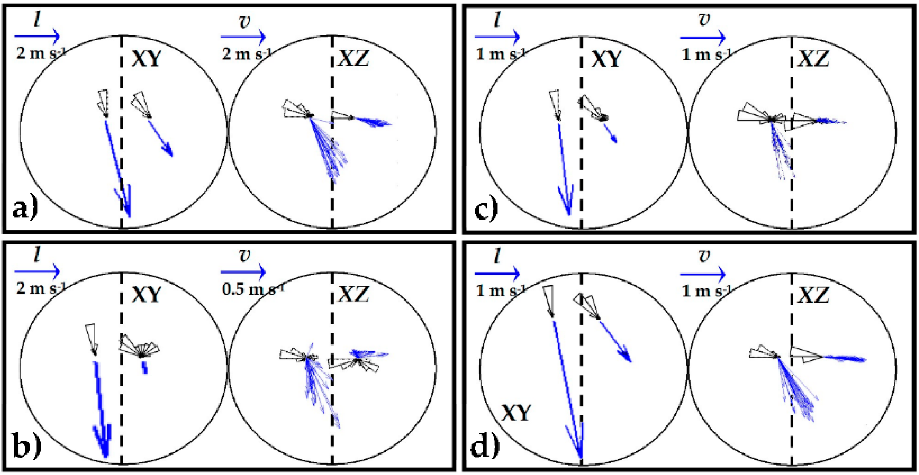
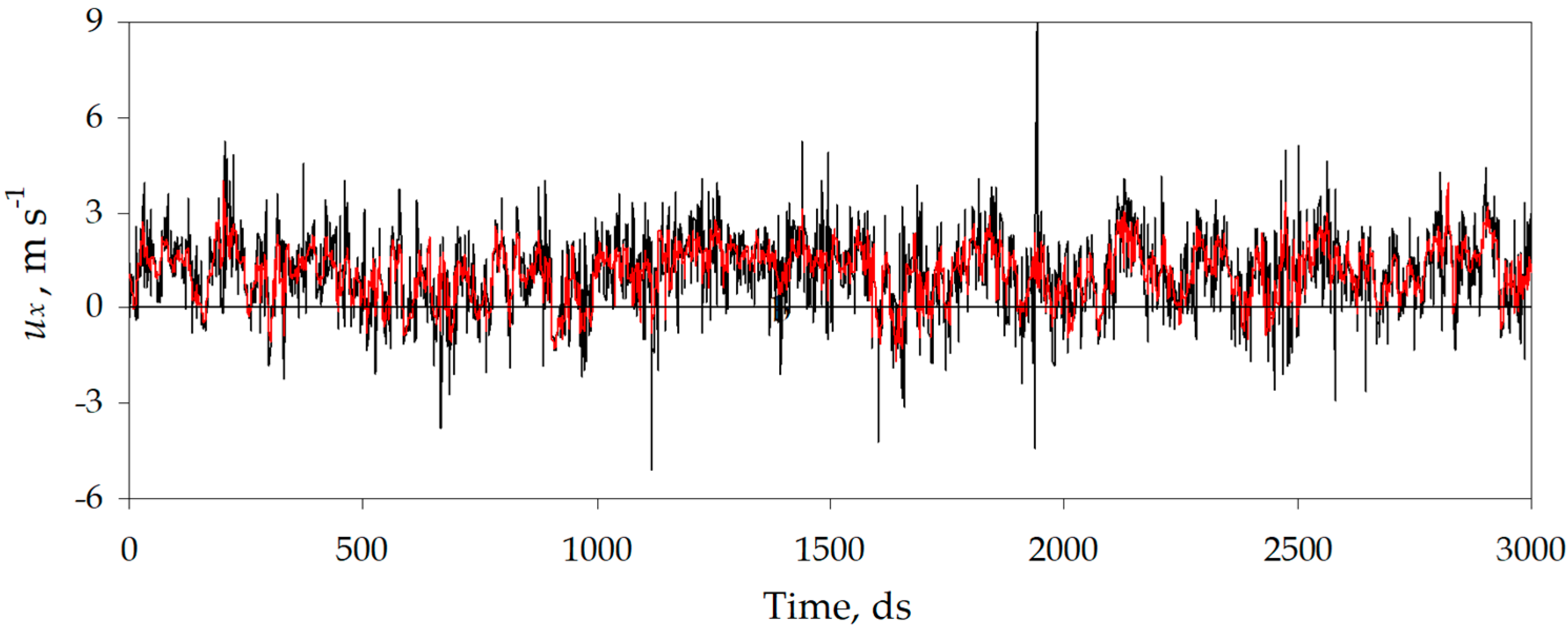
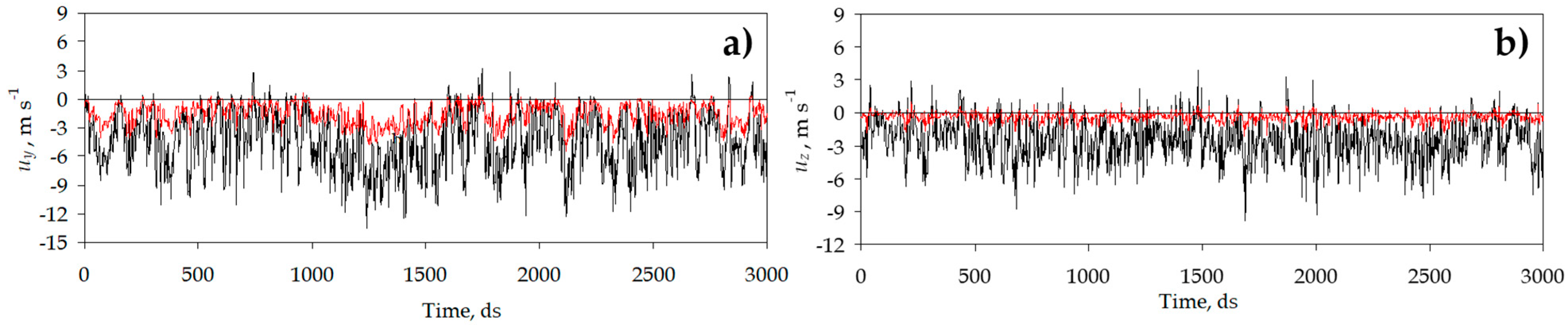
The porous IPS acts as a filter mainly for the u_x component, as it reduces part of the large fluctuations, while the lower variations are kept around the mean value (see Figure 5). On the other hand, for the transversal and vertical components (see Figure 6), in addition, to eliminate part of the large fluctuations, it considerably reduces the mean value of these components. This is reasonable because the size of the pores can filter only larger velocity fluctuations, and as the size of the pore increases (and actually the porosity), the filtering may be less noticeable. Thus, the filtering effect in u_y and u_z is directly related to the reduction of the turbulence scales for the said components after passing through the IPS (

Table 5. Macroscale L_i [m] and microscale λ [m] (longitudinal component, L_ix; transversal component, L_iy; vertical component, L_iz).

Test		Li	Lix	Liy	Liz	λ	λx	λy	λz
1	Inside	3.17	1.67	2.57	5.57	0.04	0.32	0.44	0.04
	Outside	9.61	0.92	6.07	8.85	0.36	0.13	0.99	0.36
2	Inside	0.12	0.08	0.13	0.37	0.08	0.02	0.03	0.02
	Outside	3.36	0.10	2.48	2.32	0.43	0.01	0.34	0.06
3	Inside	0.52	0.47	0.47	0.15	0.24	0.13	0.08	0.00
	Outside	2.94	0.23	2.23	2.54	0.67	0.03	0.53	0.14
4	Inside	2.47	1.43	2.19	2.85	0.73	0.33	0.37	0.01
	Outside	9.62	0.65	6.93	10.71	1.12	0.08	1.01	0.21

). In this table, the macroscale (average size of the largest eddies) and microscale (average size of the smallest eddies) parameters are given (including also their three components) for the turbulence inside and outside the window sides observing a dramatical reduction in turbulence.

As also observed by other researchers, the use of a high-density IPS, such as the one studied in this work, reduces turbulence dramatically, whilst the spectral decay rate is increased. This is observed by a transition to smaller turbulence flow scales, which are less energetic and dissipative in the evacuation of heat and mass from the greenhouse [2]. Thus, providing additional information on the characteristics of the turbulence filtering of IPS as performed in the present work is essential since the larger the size of the eddies, the more dominant the turbulent mixing, and hence the more efficient the ventilation is. Furthermore, as pointed out in Tanny et al. [29], to find the potential relations between the turbulent scales and the geometric parameters of the IPS is of significant interest in the design of efficient, low-cost, and sustainable natural ventilation systems.

The effect on the scales of the turbulence of the IPS is different according to the orthogonal component of the air velocity considered. The structure of the IPS causes the breaking of the turbulence scales for the transverse component (L_iy and λ_y) and the vertical component (L_iz and λ_z), while an increase in the turbulence scales of the longitudinal component (L_ix and λ_x) (Table 5). This increase in the turbulence scale may be the consequence of the grid-generated effect on turbulence, which is adopted in many fluid dynamics experiments to generate turbulent flows by passing laminar flows through grids [46,55]. More specifically, for u_y and u_z, at each pore, there are top–bottom and left–right threads contributing to the filtering. However, for u_x, two scenarios take place together: small eddies can pass through the pore with minimal perturbations, and larger eddies may split or break due to the presence of the threads, leading quicker to smaller eddies entering the greenhouse. Thus, the macroscale of the longitudinal component L_ix can increase up to 220% on the inner face of the window and the microscale λ_x up to 429% (Test 4). On the contrary, for the other two components, the macroscale is reduced by an average of 75% and 72% for the transversal component L_iy and vertical L_iz, respectively. Likewise, the microscale is reduced by an average of 74% and 87% for λ_y and λ_z, respectively. The increase in the longitudinal component of the turbulence scale and decrease in the transversal and vertical components has also been noticed by Teitel et al. [16]. Although they characterized turbulence inside the greenhouse and not near the IPSs, they noticed the same behavior mainly due to the top bound and side bounds of the canopy. In our case, the threads also create lateral and top bounds that constrain the airflow, but not in the longitudinal motion, hence the here shown observation.

The main drawback from the use of IPSs is the reduction of the turbulent kinetic energy, k, and the energy dissipation rate, ε. The most relevant and useful characteristic of turbulence flows in natural ventilation is the ability of turbulent flows to mix and transport heat and water vapor [28,29]. This is mainly attributed to the turbulence kinetic energy: the higher the k, the more efficient the heat and mass transfer. Unfortunately, the use of IPSs on the greenhouse window drastically reduced such turbulence kinetic energy levels, with an average reduction in turbulence kinetic energy k of 95%, but even reaching reductions of up to 99.97% (Test 2). The dissipation rate was also reduced (average reduction of 99.9%).

The energy levels observed on the outer face of the side window are similar to the values observed by Boulard et al. [56] inside a screenless tunnel greenhouse, with k values greater than 1.44 m² s⁻², and ε greater than 1.44 m² s⁻³ in the lateral windward ventilation openings. Similar facts were observed in the macroscale. They indicated maximum values of L_ix equal to 8.37 m, L_iy equal to 3.76 m, and L_iz equal to 2.07 m in the windward-oriented window.

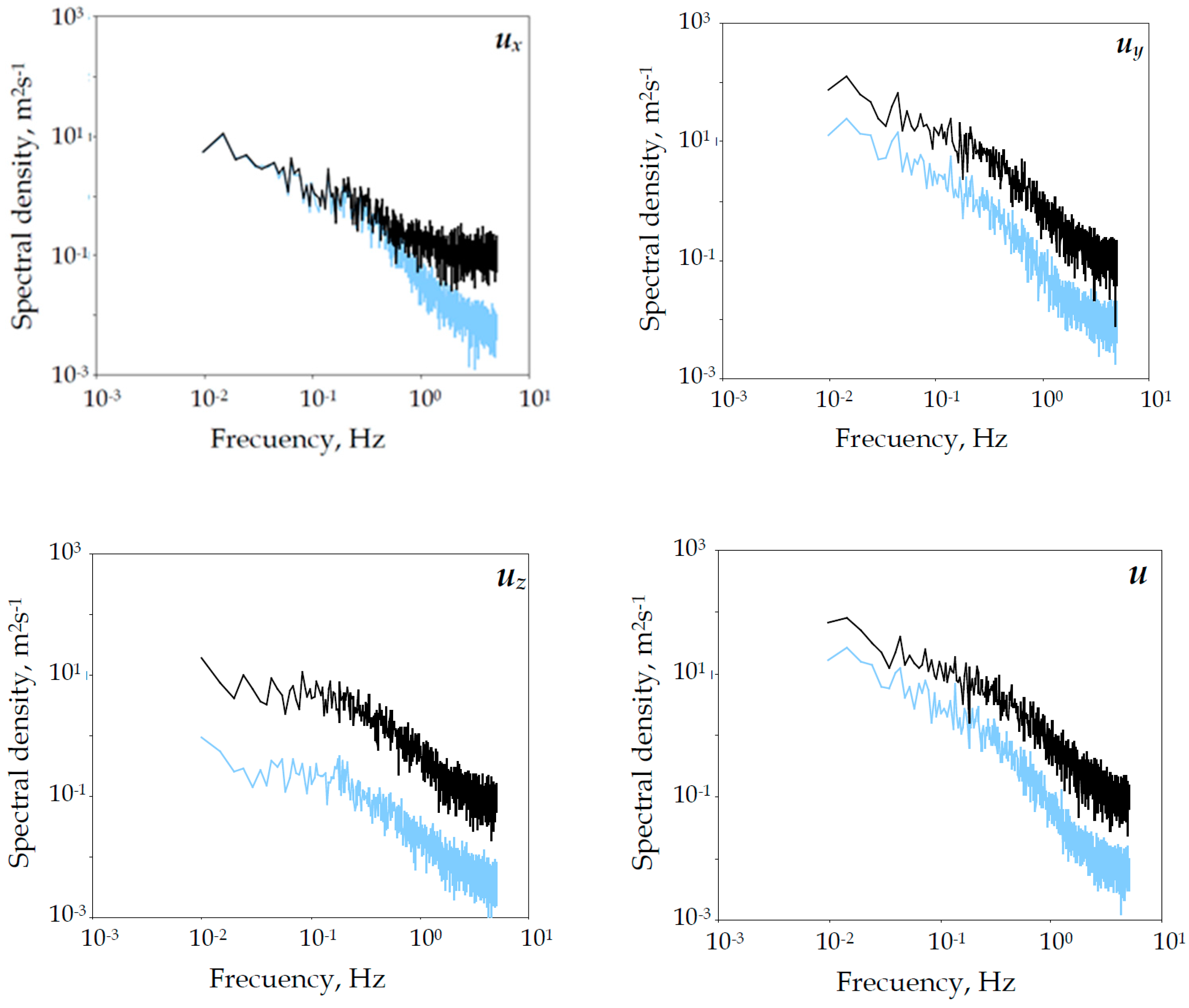
The reduction in energy suffered after passing through the IPS is clearly observed in the plot of the energy density spectra on the inner and outer faces of the window. Teitel and Tanny [27] used a one-dimensional sonic anemometer to certify that the use of a high-mesh IPS leads to a reduction in turbulence levels and scales and an increase in the spectral decay rate. However, since they used a one-dimensional anemometer, they could not observe the effect on each airflow vector field component. In the present investigation, 3D sonic anemometers have been used, being possible to observe that the impact on each component is not the same. Spectra of the velocity components were calculated using detrended records of the 30 min data acquired by a sonic anemometer at a sampling rate of 10 Hz. The 30 min period was subdivided into six consecutive sections of 5 min, each with 3000 data points. A spectrum was calculated for each section, and the six resulting values were averaged. The results for each velocity component and total velocity are shown in Figure 7.

From Figure 7, interesting observations can be made. In the transversal and vertical components u_y and u_z, turbulence energy is reduced throughout the entire frequency range. However, in the longitudinal component u_x, the energy transported in the larger scales (at low frequency) is maintained after passing through the mesh, whereas the energy transported by the smaller scales (high frequency) is dissipated or lost when passing through the porous mesh. For the total airflow velocity u, the results obtained agree with the observations made by Teitel and Tanny [27], which confirms that the turbulence energy decreases and the spectral decay rate is increased. It is obvious that this loss of energy at high frequency is what produces the reduction in the velocity fluctuations of u_x (seen in Figure 5). Regarding the other two components, the turbulence energy at low and high frequencies is reduced, which results in a decrease in the average airspeed and also in fluctuations (Figure 6). The passage of air through the mesh pores also causes a generalized increase in the slope of the spectrum (see

Table 6. Spectral decay slope β (slope in the longitudinal component, β_x; transversal component, β_y; vertical component, β_z).

Test		β	βx	βy	βz
1	Inside	1.58	1.45	1.55	1.08
	Outside	1.28	0.63	1.36	1.12
2	Inside	1.40	2.13	1.83	1.85
	Outside	1.37	0.59	1.55	1.33
3	Inside	1.53	1.82	1.59	1.31
	Outside	1.37	0.66	1.47	1.21
4	Inside	1.76	1.69	1.67	1.21
	Outside	1.36	0.65	1.53	1.25

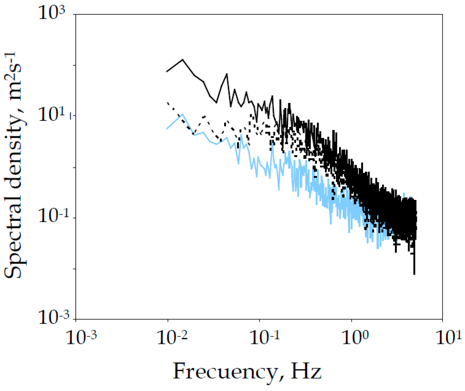
and Figure 7) [2]. A greater slope of the spectrum indicates a greater distribution of energy in the larger scales (lower frequencies). In addition, if the three spectral density plots are matched, it can be observed that the one corresponding to u_x is less energetic (Figure 8). Most of the airflow turbulence energy is transported in the transverse and vertical components. An important part of such energy is lost as discussed above, either when passing through the mesh or because of the air rejection due to the barrier created by the IPS threads, perhaps even avoiding part of the mass-flow rate to enter into the greenhouse as part of the flow may be deviated by the screen.

4. Conclusions

The present investigation focused on the analysis of the impact of the use of 13 × 30 threads·cm⁻² insect-proof screen (IPS) on the turbulence properties of the airflow, as IPSs represent an important physical barrier to insects but also to efficient natural ventilation in greenhouses.

Four independent tests were performed in the study. Much of the outside airflow approaching the side windows is deflected transversely or vertically without passing through the windows. Thus, the total air velocity u is reduced on average by 71% when entering into the greenhouse through the windward oriented side window. Due to this flow deviation, the transversal u_y and vertical u_z components are reduced by 76% and 88%, respectively. However, the observed variations of the longitudinal component u_x, perpendicular to the lateral window, are mainly due to the separation of the anemometers with respect to the window placed at the same position in the four tests. Furthermore, reduction in air velocity caused by the presence of the IPS may occur, mainly due to preventing the passage of air currents or flows that are not directed perpendicular to the window cross-surface (i.e., to the pore section of the mesh).

The IPS acts as a filter for the u_x component, eliminating part of the magnitude of the large fluctuations while keeping the lower variations around the mean value. In addition, the transverse and vertical components considerably reduce the mean value since the physical barrier created by the screen slows down the airflow velocity component that has not arrived with enough perpendicularity to the window surface plane.

The use of the IPS in the greenhouse windows drastically reduces the levels of turbulent kinetic energy k of the airflow by 95% and may up to 99.97%. The energy density spectra allow the visualization of the reduction in the turbulence energy of the airflow after passing through the IPS. For the transversal u_y and vertical u_z components, the energy is reduced throughout the entire frequency range. However, for the longitudinal component u_x, the energy transported by the larger scales is maintained after passing through the mesh, whereas the energy transported by the smaller scales is highly dissipated or lost. The use of classic natural ventilation systems as windows with installed IPSs represents a very important barrier to the benefits of using turbulent airflows for ventilation. Providing details on the impact of screens on the turbulence properties of ventilation airflows is vital for commercial distribution. In addition, gaining more knowledge on the impact of the installation of IPSs is important in order to deliver and develop better and more suitable IPSs. Thus, future work involves finding the potential relations between the turbulent scales and the geometric parameters of the IPS since this can lead to the design of more efficient, low-cost, and sustainable natural ventilation systems. The performance of turbulence models in CFD simulations can be validated with the present experimental results. Once simulations are validated, many new designs can be tested computationally in order to find optimal IPS designs.

References

1. Agrafioti, P.; Faliagka, S.; Lampiri, E.; Orth, M.; Pätzel, M.; Katsoulas, N.; Athanassiou, C.G. Evaluation of silica-coated insect proof nets for the control of Aphis fabae, Sitophilus oryzae, and Tribolium confusum. Nanomaterials 2020, 10, 1658. [Google Scholar] [CrossRef] [PubMed]
2. Teitel, M. The effect of screened openings on greenhouse microclimate. Agric. For. Meteorol. 2007, 143, 159–175. [Google Scholar] [CrossRef]
3. Oliva, R.M.; Álvarez, A.J. Factors influencing the efficacy of insect-proof screens. Acta Hortic. 2017, 1170, 1027–1033. [Google Scholar] [CrossRef]
4. Berlinger, M.J.; Leblush-Mordechl, S.; Fridja, D.; Mor, N. The effect of types of greenhouse screens on the presence of western flower thrips: A preliminary study. OILB-SROP Bull. 1992, 16, 13–19. [Google Scholar]
5. Taylor, R.A.J.; Shalhevet, S.; Spharim, I.; Berlinger, M.J.; Lebiush-Mordechi, S. Economic evaluation of insect-proof screens for preventing tomato yellow leaf curl virus of tomatoes in Israel. Crop Prot. 2001, 20, 561–569. [Google Scholar] [CrossRef]
6. Bethke, J.A.; Paine, T.D. Screen hole size and barriers for exclusion on insect pest of glasshouse crops. J. Entomol. Sci. 1991, 26, 169–177. [Google Scholar] [CrossRef]
7. Verheye, P.; Verlodt, H. Comparison of different systems for static ventilation of hemispheric plastic greenhouses. Acta Hortic. 1990, 281, 183–197. [Google Scholar] [CrossRef]
8. Von Zabeltitz, C. L’efficacité énergétique dans la conception des serres méditerranéennes. Plasticulture 1992, 96, 6–16. [Google Scholar]
9. ANSI/ASAE. EP406.1: Heating, Ventilating, and Cooling Greenhouses; ASAE: St. Joseph, MI, USA, 1994. [Google Scholar]
10. Kittas, C.; Boulard, T.; Papadakis, G. Natural ventilation of a greenhouse with ridge and side openings: Sensitivity to temperature and wind effects. Trans. ASAE 1997, 40, 415–425. [Google Scholar] [CrossRef]
11. Kittas, C.; Katsoulas, N.; Bartzanas, T.; Mermier, M.; Boulard, T. The impact of insect screens and ventilation openings on the greenhouse microclimate. Trans. ASABE 2008, 51, 2151–2165. [Google Scholar] [CrossRef]
12. Formisano, L.; El-Nakhel, C.; Corrado, G.; De Pascale, S.; Rouphael, Y. Biochemical, physiological, and productive response of greenhouse vegetables to suboptimal growth environment induced by insect nets. Biology 2020, 9, 432. [Google Scholar] [CrossRef] [PubMed]
13. López-Martínez, A.; Martínez, D.L.V.; Aiz, F.D.M.; Peña, A.; Membrive, P.M. Microclimate evaluation of a new design of insect-proof screens in a Mediterranean greenhouse. Span. J. Agric. Res. 2014, 2, 338–352. [Google Scholar] [CrossRef] [Green Version]
14. Harmanto; Tantau, H.J.; Salokhe, V.M. Microclimate and air exchange rates in greenhouses covered with different nets in the humid tropics. Biosyst. Eng. 2006, 94, 239–253. [Google Scholar] [CrossRef]
15. Yang, G.; Guo, Z.; Ji, H.; Sheng, J.; Chen, L.; Zhao, Y. Application of insect-proof nets in pesticide-free rice creates an altered microclimate and differential agronomic performance. PeerJ 2018, 6, e6135. [Google Scholar] [CrossRef] [Green Version]
16. Teitel, M.; Liang, H.; Vitoshkin, H.; Tanny, J.; Ozer, S. Airflow patterns and turbulence characteristics above the canopy of a tomato crop in a roof-ventilated insect-proof screenhouse. Biosyst. Eng. 2020, 190, 184–200. [Google Scholar] [CrossRef]
17. Bartzanas, T.; Boulard, T.; Kittas, C. Numerical simulation of the airflow and temperature distribution in a tunnel greenhouse equipped with insect-proof screen in the openings. Comput. Electron. Agric. 2002, 34, 207–221. [Google Scholar] [CrossRef]
18. Fatnassi, H.; Boulard, T.; Demrati, H.; Bouirden, L.; Sappe, G. Ventilation Performance of a Large Canarian-Type Greenhouse equipped with Insect-proof Nets. Biosyst. Eng. 2002, 82, 97–105. [Google Scholar] [CrossRef]
19. Fatnassi, H.; Boulard, T.; Bouirden, L. Simulation of climatic conditions in full-scale greenhouse fitted with insect-proof screens. Agric. For. Meteorol. 2003, 118, 97–111. [Google Scholar] [CrossRef]
20. Fatnassi, H.; Boulard, T.; Poncet, C.; Chave, M. Optimisation of greenhouse insect screening with computational fluid dynamics. Biosyst. Eng. 2006, 93, 301–312. [Google Scholar] [CrossRef]
21. Baeza, E.J.; Pérez-Parra, J.J.; Montero, J.I.; Bailey, B.J.; López, J.C.; Gázquez, J.C. Analysis of the role of sidewall vents on buoyancy-driven natural ventilation in parral-type greenhouses with and without insect screens using computational fluid dynamics. Biosyst. Eng. 2009, 104, 86–96. [Google Scholar] [CrossRef]
22. Teitel, M.; Barak, M.; Berlinger, M.J.; Lebiush-Mordechai, S. Insect-proof screens in greenhouses: Their effect on roof ventilation and insect penetration. Acta Hortic. 1999, 507, 25–34. [Google Scholar] [CrossRef]
23. López, A.; Martínez, D.L.V.; Aiz, F.D.M.; Peña, A. Sonic anemometry measurements to determine airflow patterns in multi-tunnel greenhouses. Span. J. Agric. Res. 2012, 3, 631–642. [Google Scholar] [CrossRef] [Green Version]
24. López-Martínez, A.; Molina-Aiz, F.D.; Valera, D.L.; Peña, A. Wind tunnel analysis of the airflow through insect-proof screens and comparison of their effect when installed in a Mediterranean greenhouse. Sensors 2016, 16, 690. [Google Scholar] [CrossRef] [PubMed] [Green Version]
25. López-Martínez, A.; Molina-Aiz, F.D.; Valera, D.L.; Espinoza-Ramos, K.E. Models for characterising the aerodynamics of insect-proof screens from their geometric parameters. Biosyst. Eng. 2020, 192, 42–55. [Google Scholar] [CrossRef]
26. Granados-Ortiz, F.-J.; Arrabal-Campos, F.M.; Lopez-Martinez, A.; Molina-Aiz, F.D.; Peña-Fernández, A.; Valera-Martínez, D.L. On the estimation of three-dimensional porosity of insect-proof screens. Comput. Electron. Agric. 2022. in Press. [Google Scholar] [CrossRef]
27. Teitel, M.; Tanny, T. Heat Fluxes and Airflow Patterns Through Roof Windows in a Naturally Ventilated Enclosure. Flow Turbul. Combust. 2005, 74, 21–47. [Google Scholar] [CrossRef]
28. Pope, S.B. Turbulent Flows; Cambridge University Press: Cambridge, UK, 2000. [Google Scholar]
29. Tanny, J.; Haslavsky, V.; Teitel, M. Airflow and heat flux through the vertical opening of buoyancy-induced naturally ventilated enclosures. Energ. Build. 2008, 40, 637–646. [Google Scholar] [CrossRef]
30. Valera, D.L.; Álvarez, A.J.; Molina-Aiz, F.D. Aerodynamic analysis of several insect-proof screens used in greenhouses. Span. J. Agric. Res. 2006, 4, 273–279. [Google Scholar] [CrossRef]
31. Shilo, E.; Teitel, M.; Mahrer, Y.; Boulard, T. Air-flow patterns and heat fluxes in roof-ventilated multi-span greenhouse with insect-proof screens. Agric. For. Meteorol. 2004, 122, 3–20. [Google Scholar] [CrossRef]
32. Von Karman, T. Some remarks on the statistical theory of turbulence. In Proceedings of the fifth International Congress for Applied Mechanics, Cambridge, MA, USA, 12–16 September 1938; p. 347. [Google Scholar]
33. Hinze, J.O. Turbulence; McGraw-Hill: New York, NY, USA, 1975. [Google Scholar]
34. Chapman, G.T.; MTobak, M. Observations, Theoretical Ideas, and Modeling of Turbulent Flows—Past, Present and Future. In Theoretical Approaches to Turbulence; Dwoyer, D.L., Hussaini, M.Y., Voigt, R.G., Eds.; Springer: New York, NY, USA, 1985; pp. 19–49. [Google Scholar]
35. Gustavsson, H. Lecture notes: Introduction to turbulence. In Luleå: Division of Fluid Mechanics; Luleå University of Technology: Luleå, Sweden, 2006. [Google Scholar]
36. Cebeci, T. Analysis of Turbulent Flows; Elsevier Science: Amsterdan, The Netherlands, 2004. [Google Scholar]
37. Heber, A.J.; Boon, C.R.; Peugh, M.W. Air patterns and turbulence in an experimental livestock building. J. Agric. Eng. Res. 1996, 64, 209–226. [Google Scholar] [CrossRef] [Green Version]
38. Maryami, R.; Showkat Ali, S.A.; Azarpeyvand, M.; Afshari, A. Turbulent flow interaction with a circular cylinder. Phys. Fluids 2020, 32, 015105. [Google Scholar] [CrossRef] [Green Version]
39. Mora, D.O.; Obligado, M. Estimating the integral length scale on turbulent flows from the zero crossings of the longitudinal velocity fluctuation. Exp. Fluids 2020, 61, 199. [Google Scholar] [CrossRef]
40. O’Neill, P.L.; Nicolaides, D.; Honnery, D.; Soria, J. Autocorrelation functions and the determination of integral length with reference to experimental and numerical data. In Proceedings of the 15th Australasian Fluid Mechanics Conference, Sydney, NSW, Australia, 13–17 December 2004; Volume 1, pp. 1–4. [Google Scholar]
41. Melikov, A.K.; Langkilde, G.; Derbiszewski, B. Airflow characteristic in the occupied zone of rooms with displacement ventilation. ASHRAE Trans. 1990, 96, 555–563. [Google Scholar]
42. Shen, Z.; Zhang, X. Random-eddy-superposition technique for leading edge noise predictions. In Proceedings of the 2018 AIAA/CEAS Aeroacoustics Conference, Atlanta, Georgia, 25–29 June 2018; p. 3597. [Google Scholar]
43. Hamba, F. Turbulent energy density in scale space for inhomogeneous turbulence. J. Fluid Mech. 2018, 842, 532–553. [Google Scholar] [CrossRef]
44. Ouyang, Q.; Dai, W.; Li, H.; Zhu, Y. Study on dynamic characteristics of natural and mechanical wind in built environment using espectral analisis. Build. Environ. 2006, 41, 418–426. [Google Scholar] [CrossRef]
45. Stull, R.B. An Introduction to Boundary Layer Meteorology; Kluwer Academics Publishers: Dordrecht, The Netherlands, 1988. [Google Scholar]
46. Laizet, S.; Nedić, J.; Vassilicos, J.C. The spatial origin of −5/3 spectra in grid-generated turbulence. Phys. Fluids 2015, 27, 065115. [Google Scholar] [CrossRef] [Green Version]
47. Loomans, M.G.L.C. The Measurement and Simulation of Indoor Air Flow. Master’s Thesis, Technische Universiteit Eindhoven, Eindhoven, The Netherlands, 1998. [Google Scholar]
48. Ting, D. Basics of Engineering Turbulence; Academic Press: Cambridge, MA, USA; Elsevier: Amsterdam, The Netherlands, 2016. [Google Scholar]
49. Abou-Hweij, W.; Azizi, F. CFD simulation of wall-bounded laminar flow through screens. Part I: Hydrodynamic characterization. Eur. J. Mech.-B/Fluids 2020, 84, 207–232. [Google Scholar] [CrossRef]
50. Muñoz, P.; Montero, J.I.; Antón, A.; Giuffrida, F. Effect of insect-proof screens and roof openings on greenhouse ventilation. J. Agric. Eng. Res. 1999, 73, 171–178. [Google Scholar] [CrossRef]
51. Teitel, M. The effect of insect-proof screens in roof openings on greenhouse microclimate. Agric. For. Meteorol. 2001, 110, 13–25. [Google Scholar] [CrossRef]
52. Molina-Aiz, F.D.; Valera, D.L.; Peña, A.A.; Gil, J.A.; López, A. A Study of Natural Ventilation in an Almería-Type Greenhouse with Insect Screens by Means of Tri-sonic Anemometry. Biosyst. Eng. 2009, 104, 224–242. [Google Scholar] [CrossRef]
53. Fang, F. A design method for contractions with square end sections. Trans. ASME 1997, 119, 454–458. [Google Scholar] [CrossRef]
54. Fang, F.; Chen, J.C.; Hong, Y.T. Experimental and analytical evaluation of flow in a square-to-square wind tunnel contraction. J. Wind Eng. Ind. Aerodyn. 2001, 89, 247–262. [Google Scholar] [CrossRef]
55. Melina, G.; Bruce, P.J.; Vassilicos, J.C. Vortex shedding effects in grid-generated turbulence. Phys. Rev. Fluids 2016, 1, 044402. [Google Scholar] [CrossRef] [Green Version]
56. Boulard, T.; Wang, S.; Haxaire, R. Mean and turbulent air flows and microclimatic patterns in an empty greenhouse tunnel. Agric. For. Meteorol. 2000, 100, 169–181. [Google Scholar] [CrossRef]
Figure 1. Sketch of the halved greenhouse for the experimental tests.
Agronomy 12 00586 g001
Figure 2. Detail of the IPS under study: (a) Microscope image of the insect-proof screen (IPS) under analysis (density: 13 × 30 threads·cm−2), and (b) Computational reconstruction of the 3D shape using Poro3D software [26], where warp threads are shown in red color, and the weft threads in blue color.
Agronomy 12 00586 g002
Figure 3. Sketch of the setup of the 3D anemometers placed at the side vent north.
Agronomy 12 00586 g003
Figure 4. Representation of the airflow on the outer and inner face of the north side window facing windward. Tests 1 (a), 2 (b), 3 (c) and 4 (d). Representation of the global mean vector for the XY plane and minute mean vectors for the XZ plane.
Agronomy 12 00586 g004
Figure 5. Three-dimensional sonic anemometry ux measurements from Test 1 at the side window windward oriented. Inner side of the IPS at the window (); outer side of the IPS at the window (▬). Total acquisition time: Five minutes.
Agronomy 12 00586 g005
Figure 6. Three-dimensional sonic anemometry measurements from Test 1 at the side window windward oriented. The measurements correspond to the transversal component uy (a), and vertical component uz (b). Inner side of the IPS at the window (); outer side of the IPS at the window (▬). Total acquisition time: Five minutes.
Agronomy 12 00586 g006
Figure 7. Energy density spectra at the north side window (Test 1). Outer window side (▬) and inner window side ().
Agronomy 12 00586 g007
Figure 8. Energy density spectra at outer window side at the north side window (Test 1). Spectra of ux (), uy (▬), and uz ( Agronomy 12 00586 i001).
Agronomy 12 00586 g008