Comparison of Methane Emission Patterns from Dairy Housings with Solid and Slatted Floors at Two Locations

Abstract

Methane (CH${}_4$) emissions from dairy husbandry are a hot topic in the context of active climate protection, where housing systems with slatted floors and slurry storage inside are in general expected to emit more than systems with solid floors. There are multiple factors, including climate conditions, that modulate the emission pattern. In this study, we investigated interrelations between CH${}_4$ emission patterns and climate conditions as well as differences between farm locations versus floor effects. We considered three data sets with 265, 264 and 275 hourly emission values from two housing systems (one slatted, one solid floor) in Switzerland and one system with solid floors in Germany. Each data set incorporated measurements in summer, winter and a transition season. The average CH${}_4$ emission was highest for the slatted floor system. For the solid floor systems, CH${}_4$ emissions at the Swiss location were around 30% higher compared to the German location. The shape of the distributions for the two solid floor systems was rather similar but very different from the distribution for the slatted floor system, which showed higher prevalence for extreme emissions. Rank correlations, which measure the degree of similarity between two rankings in terms of linear relation, were not able to detect dependencies at the selected significance level. In contrast, mutual information, which measures more general statistical dependencies in terms of shared information, revealed highly significant dependencies for almost all variable pairs. The weakest statistical relation was found between winds speed and CH${}_4$ emission, but the convection regime was found to play a key role. Clustering was consistent among the three data sets with five typical clusters related to high/low temperature and wind speed, respectively, as well as in some cases to morning and evening hours. Our analysis showed that despite the disparate and often insignificant correlation between environmental variables and CH${}_4$ emission, there is a strong relation between both, which shapes the emission pattern in many aspects much more in addition to differences in the floor type. Although a clear distinction of high and low emission condition clusters based on the selected environmental variables was not possible, trends were clearly visible. Further research with larger data sets is advisable to verify the detected trends and enable prognoses for husbandry systems under different climate conditions.

1. Introduction

One of the great challenges of our century is to take action to combat climate change and its impacts, as it is verbalized in the thirteenth sustainable development goal of the United Nations (https://sdgs.un.org/goals, last access 20 December 2021). Regional and local impacts of the continuing global warming trend have already become apparent and highlight the urgent need for adaptation and greenhouse gas mitigation measures in all economic sectors, including agriculture [1,2,3,4]. On the other hand, in terms of agriculture, the global economic development and population growth resulted in continuously increasing demand for food, where a substantial part is currently covered by animal-based products [5,6]. At the same time, livestock production is a substantial source of air pollution in terms of ammonia and greenhouse gases.

With regard to greenhouse gases, methane (CH${}_4$) is a substance of particular importance and complexity regarding its emission process. The Food and Agricultural Organization (FAO) of the United Nations estimated in 2013 that nearly half of the greenhouse gas emissions from the livestock sector are in the form of CH${}_4$, while nitrous oxide and carbon dioxide contribute about 28% each [7]. Moreover, dairy cattle husbandry contributed around 20% of the total greenhouse gas emissions from the livestock sector by that time. In addition, according to recent estimates of the global CH${}_4$ budget for 2017, around 30% of the total anthropogenic CH${}_4$ emissions originate from enteric fermentation and manure [8]. Therefore, CH${}_4$ emissions from dairy husbandry are a hot topic among farmers, society and stakeholders in the context of active climate protection. Freestalls and loose housings with cubicles are the most common housing systems in many parts of the world [9]. In most European countries, naturally ventilated housings (NVH) with cubicles play an important role in dairy husbandry (e.g., [10,11,12,13]). In these systems, the indoor climate is strongly related to the outdoor weather conditions, which has implications for pollutant emissions in general. NVHs with cubicles can be further subdivided with respect to floor types: solid floors or slatted floors [12]. According to measurements and modeling in a loose housing with cubicles and solid floors in the study by Ngwabie et al., around 81% of the CH${}_4$ emissions originate from enteric fermentation and about 19% is manure-based [14]. Similarly, Dutch CH${}_4$ emission data show that enteric fermentation is responsible for roughly 80% of the CH${}_4$ emissions from cattle housings [15]. Whereby Monteny et al. assumed that the proportion of slurry-based CH${}_4$ emissions could be higher in housing systems with perforated floors and slurry storage inside the housing compared to systems with solid floors. Furthermore, both enteric and slurry-based CH${}_4$ emissions can be modulated by multiple factors, such as breed, diet, feeding routines, animal activity, climate conditions, etc. (e.g., [12,16,17,18,19,20,21]). In contrast, to other emitted air pollutants (e.g., ammonia) the effect of meteorological variables, such as temperature and wind speed, on the emission process of methane is not conclusively explained in the literature. On the one hand, this is related to the complex physiological and behavioral reactions to ambient climate affecting the metabolism of ruminants and, thereby, likely the enteric fermentation also [22]. On the other hand, if the wind speed near the active emission surface increases, the thickness of the boundary layer between liquid manure and the atmosphere and, in consequence, the resistance for diffusive gas transfer decreases, resulting in higher local emissions [23]. The literature on the temperature effect on methane emissions from manure is partly contradictory. In general, CH${}_4$ emissions from manure are expected to increase with increasing temperature, and thus, cooling liquid manure is considered to be a CH${}_4$ mitigation measure [16,24]. However, in an experiment conducted in a dairy housing with slatted floors, a slight decrease in averaged CH${}_4$ emissions was found at increased temperature, whereas the mean temperature per measuring phase ranged from 4 to 15 ${}^{\circ }$C [25]. A notable increase in slurry-based CH${}_4$ emissions has been reported in the literature for temperatures above about 15 ${}^{\circ }$C [26]. However, if the temperature falls below a certain threshold for some time, the subsequent methane emission does not substantially increase anymore with raising temperatures, even for temperatures above the threshold [27]. In consequence, so far it is not conclusively clarified which combination of factors leads to particularly high or low CH${}_4$ emission values.

Correlation analysis is a common tool to identify potential relationships between measurands or model predictions in many research disciplines, including agriculture. In agricultural and environmental studies, it has been used, for example, to link exposure to pesticides and adverse health effects, to explore whether emission values are related to distinct features, or to compare the emission predictions of different modeling approaches [13,28,29,30,31,32]. In many applications, this kind of statistical analysis relies on the widely known Pearson correlation coefficient, which has, however, three major limitations with regard to its applicability [33]: (i) It is based on the assumption that the underlying distributions of the measured variables are normally distributed, i.e., the frequency distribution is approximately Gaussian with vanishing statistical moments of third and higher order. (ii) It focuses on linear relationships and ignores many other types of relationships, i.e., in particular, nonlinear relations might be misinterpreted as independent variables. (iii) It investigates only pairwise relations.

Alternatives are rank correlations, mutual information and cluster analysis, which are less common in agricultural and environmental studies. Rank correlation is a non-parametric equivalent to Pearson correlation. It measures how well any monotonic function describes the relation between two measurands. In this sense, rank correlations such as Spearman’s rho or Kendall’ tau overcome the first of the above-mentioned issues [34,35]. Mutual information is an information-theoretic measure that assesses the strength of an arbitrary statistical relation between two variables [36,37]. A vanishing mutual information means statistical independence. This measure is not restricted to linear relations and can thus overcome the first two issues with the Pearson correlation indicated above. However, mutual information is not normalized as a correlation, i.e., further statistics are required to define what is non-vanishing mutual information for a particular case. Clustering is an unsupervised machine learning technique to group data points that have similar properties and/or features [38]. Similarity measures such as the Euclidian distances are often used to distinguish cluster affiliations. Cluster analysis is usually intended for dimensionality reduction in large data sets. It does not rely on assumptions on the frequency distribution of the involved data or any linear relationships and can consider multiple variables at a time. In this context, it can also be useful to identify variables that show similar dynamics and thus might be causally interrelated. All of the before-mentioned tools for time series analysis focus on different statistical aspects and differ in the degree of complexity. They are not yet standard in environmental or agricultural research. Thus, the aim of our study was to explore the potential of those tools to compare the characteristics of CH${}_4$ emission data from slatted and solid floor systems. We highlight and discuss differences and similarities in the statistical characteristics of the emissions and their dependencies on the environmental conditions for the two flooring systems. Therefore, we investigate (i) the mutual potential interrelations between CH${}_4$ emissions and meteorological variables, and (ii) the differences between farm locations versus floor effects. In this context, the term farm location incorporates all effects of farm management (including breeds, diets, feeding routines, etc.) as well as local climatic conditions and any systematic bias related to the local measurement setup. We hypothesized that despite the differences related to the farm location, the solid floor systems show a distinct emission pattern that differs considerably from the pattern of slatted floors. The patterns are shaped by environmental factors such as air temperature, wind speed and direction, as well as the time of the day. Our study was intended to obtain a better understanding of under which climatic conditions higher or lower CH${}_4$ emissions can be expected from different flooring systems. Our findings should support the further refinement of measurement and modeling strategies to project future CH${}_4$ emission values from slatted and solid floor systems for different climate situations.

2. Materials and Methods

2.1. Measurement Sites

2.1.1. Switzerland

The experimental dairy housing for emission measurement under consideration is located in north-eastern Switzerland. The building axis is orthogonal to the prevailing wind directions around south-west and north-east. The housing consists of two naturally ventilated compartments, each for 20 lactating cows equipped with three cubicle rows with straw mattresses [39]. Per compartment, the animals’ activity area with aisles and cubicles comprises an area of 16.2 × 14.1 m, of which approx. 154 m${}^2$ are longitudinal and cross aisles [40]. In the northern compartment, the longitudinal aisles were equipped with a slatted floor cleaned by a robot spraying water [41]. The southern compartment has a solid floor cleaned by an automatic manure scraper every two hours. The central area between the housing compartments contains the milking parlor and waiting area as well as technical facilities, office and analytics. The housing is designed with a mono-pitched roof, whereby the eaves height of the compartments is 4 m and the ridge height is 8.2 m. The longitudinal facades are constructed with flexible curtains and in the upper area with spaced boards. During these measurements, the cows had no access to the outdoor exercise areas or to pasture. In both compartments, the herd consisted of Brown Swiss and Swiss Fleckvieh breeds. The cows were milked twice a day at 05:30 and 16:30. They were fed a mixed ration based on grass silage, maize silage, hay, sugar beet pulp silage, protein concentrate, and mineral feed, whereby the proportions varied per season. New portions of the mixed ration were offered at 16:45 after milking. In addition, concentrates rich in energy and protein were fed by automatic concentrate feeders according to the demand of the individual animals. The experimental protocol complied with the Swiss Legislation on Animal Welfare and was approved by the Cantonal Veterinary Office of Zürich (ZH091/15).

2.1.2. Germany

The naturally ventilated barn for dairy cattle is located in North-East Germany (see, e.g., [19] or [32] for further details). A total floor area of 96.15 × 34.2 m splits up into four connected compartments and two walking aisles. The gable height is 10.73 m and the side walls height 4.2 m. The building axis is orthogonal to the main prevailing wind direction, which is nearly south. The long sidewalls are equipped with wind-breaking nets and adjustable curtains. The gable walls incorporate space boards and doors with adjustable curtains as well as a gate each (approx. 16 m${}^2$ in size). The barn had straw-bedded cubicles to accommodate around 370 Holstein-Frisian cows in four groups. The solid concrete aisle floors were cleaned by automatic scrapers every 1.5 h. Cows went out for milking group-wise for about 1 h three times a day. A milking cycle for the whole barn took about 4.5 h. The three milking cycles started approximately at 06:00 a.m., 02:00 p.m. and 10:00 p.m. Feed was provided around 06:45 a.m. and 10:30 a.m. as a total mixed ration consisting of maize silage, grass silage, alfalfa silage, rye silage, wheat straw, sugar beet puree, dried sugar beet pulp, sugar beet molasses, soya extraction grist, rapeseed extraction meal, maize grist, rye grist, lupine grist, further concentrates, feed lime, sodium bicarbonate, and glycerin. Feed components and amounts varied between groups and seasons.

2.2. Estimation of Ventilation Rate and Emission

The estimation of methane emission was based on the assessment of tracer dynamics in both study sites. In the Swiss study site, artificial tracers were used, while the estimation in the German study site relied on CO${}_2$ as a natural tracer. Subsequently, a normalized methane emission $ME$ was calculated by dividing by the number and average body mass of the cows and multiplying with the quantity livestock unit (LU = 500 kg body mass equivalent).

2.2.1. Artificial Tracer Approach

The emission calculation was based on the assumption that the ratio of the concentrations of emitted target gas CH${}_4$ ($MC$) and external tracer gas $TC$ corresponds to the ratio of their mass flows ($\dot{m}·{\dot{m}}_T^{-1}$). Thus, the emission (i.e., the mass flow of the target gas) can be calculated following Equation (1):

$$\dot{m}={\dot{m}}_T·MC·T{C}^{-1}$$

(1)

By multiplying with the density of the gas, the mass flow rate can be translated into a volume flow rate. The tracer ratio method, as well as its validation, is documented in the literature [39].

2.2.2. Natural Tracer Approach

The CO${}_2$ production model, published by Pedersen 2002, was used to estimate the average CO${}_2$ output per cow [42]. The estimation is based on the animal heat production at 20 ${}^{\circ }$C depending on the average body mass, the milk yield and the days in milk of the cows in the herd. This heat production and in consequence the CO${}_2$ production was corrected by the average temperature of ambient air (approximated by the measured outdoor temperature in this study).

$$Q=N·P_{C{O}_2}·\Delta C_{C{O}_2}^{-1}$$

(2)

The resulting CO${}_2$ production term $P_{C{O}_2}$ is multiplied by the number (N) of cows within the housing system and divided by the measured CO${}_2$ difference $\Delta C_{C{O}_2}$ between outgoing and incoming air in order to derive the ventilation rate Q following Equation (2). The value of the emission E was obtained by multiplying the methane concentration difference $\Delta C_{C{H}_4}$ between outgoing and incoming air (which corresponds to the background-corrected target gas concentration in the artificial tracer gas approach) with the estimated ventilation rate Q at the same time (which corresponds to the volume flow rate of the CO${}_2$).

2.3. Data Collection

The analysis in this study was based on a selection of measurements, which were conducted in the framework of two independent studies—one at the Swiss study site and one at the German study site. In the following subsections, we summarize the key parameters of the measurement setups. We further explain how data were selected from those sets of measurement data in order to homogenize the framework conditions of data collection.

2.3.1. Swiss Study Site

In order to cover the climatic variation over the year, the data collection took place in three seasons: summer (18 July 2017 to 22 July 2017), transition season (2 October 2017 to 6 October 2017) and winter (11 December 2017 to 14 December 2017).

The diluted tracer gases (ppm-range), sulfur hexafluoride (SF${}_6$) and trifluoromethylsulfur pentafluoride (SF${}_5$CF${}_3$), were dosed constantly via steel tubes equipped with critical capillaries (hole diameter 30 $\mathsf{\mu }$m, Lenox Laser Inc., Glen Arm, MD, USA) next to the aisles to mimic the emission sources. Individual tracer gases were applied in each housing compartment in order to detect any cross contamination between the two compartments. Teflon (PTFE) tubes and critical glass capillaries (hole diameter 250 $\mathsf{\mu }$m, Thermo-Instruments, Dortmund, Germany and Louwers, Hapert, The Netherlands) at the height of 2.5 m ensure a representative integrative air sample for each compartment. Background concentration of CH${}_4$ was measured about 30 m south of the housing. Concentrations of CH${}_4$ were analyzed by cavity ring-down spectroscopy (G2301; Picarro Inc., Santa Clara, CA, USA). SF${}_6$ and SF${}_5$CF${}_3$ concentrations were analyzed by gas chromatography with electron capture detection (GC-ECD, 7890A, Agilent Technologies AG, Basel, Switzerland). Details are given in Mohn et al. (2018) [39].

Wind data were measured at the height of 10 m, 60 m south-west of the housing using a three-dimensional ultrasonic anemometer (Ultra-sonic Anemometer 3D, Adolf Thies GmbH and Co. KG, Göttingen, Germany). At the same position but at the height of 2.5 m, air temperature and relative humidity was measured by a combined sensor device (temperature: PT100/PT1000 sensor; relative humidity: ROTRONIC hygrometer^®IN-1; HygroClip2, ROTRONIC AG, Bassersdorf, Switzerland).

Milk yield and consumption of concentrates were documented daily by the herd management software at the individual animal level. Live weight of each cow was determined before and after each measuring period using a measuring tape. For further analysis, we considered 265 (northern compartment) and 264 (southern compartment) hourly values of each variable.

2.3.2. German Study Site

The data set is available in the PUBLISSO repository [43]. It includes data on gas concentration (e.g., of carbon dioxide and methane), temperature and wind velocity collected between 2016-11-01 and 2017-08-30 with at least hourly resolution.

Two high-resolution Fourier Transform Infrared (FTIR) spectrometers (Gasmet CX4000, Gasmet Technologies Inc., Karlsruhe, Germany) sequentially monitored gas concentrations from ten sampling lines (four outside, six inside the building) positioned at a distance of 4 to 8 m from the walls. One of the lines was placed in the barn’s center below the roof, the other lines at 3.2 m height. Out of the four sample lines outside the building, the line with the lowest CO${}_2$ value was selected to represent outdoor gas concentrations for the background correction of CO${}_2$ and CH${}_4$ concentrations. The average of the six individual sample lines inside the building was calculated to represent the indoor concentration. All sample lines were made of Teflon tubes with an inner diameter of 6 mm and an orifice with a capillary trap every 8–10 m to ensure constant volume flow through all orifices.

Air temperature was measured at a distance of 5 m from the building with an EasyLog USB 2+ sensor (Lascar Electronics Inc., Whiteparish, UK). Wind velocity was obtained from a three-dimensional ultrasonic anemometer (Windmaster Pro ultrasonic anemometer, Gill Instruments Limited, Lymington, Hampshire, UK) at the roof of the building at about a 12 m height.

Animal data (number, mass and milk yield of cows) were provided as daily herd average by the barn’s administration.

For the analysis in this study, we selected a subset of data between 11 December 2016 and 14 December 2016, between 2 April 2017 and 6 April 2017 and between 18 July 2017 and 22 July 2017 in order to consider a similar amount of data in summer, winter and the transition season as in the other data set. Compared with the measurement dates in the Swiss data set, the spring measurements were replaced by autumn measurements. The number of measurement days was equal, while slightly more measurement hours were included than in the Swiss data set. In total, 275 hourly values of each variable were included here.

2.4. Data Analysis

We used the open source software package R version 4.0.0 for the subsequent data analysis and plotting.

2.4.1. Histograms and Statistical Moments

We used histograms to illustrate differences among the three locations in the frequency density distribution of the individual environmental variables and the CH${}_4$ emission values. In addition to this visual inspection, we calculated higher-order statistical moments in order to quantify how close or far the distributions are to/from a normal distribution (which is the underlying assumption for Pearson correlation calculation and many statistical tests). Here, we focused on the skewness and the kurtosis. Skewness is a measure of asymmetry of the distribution. A left-skewed distribution means that the tail of the distribution is longer on the left because there are more low values. In contrast, a right-skewed distribution has a longer tail at the right side of the distribution because there are more high values. Kurtosis measures the width of the tail of the distribution. A higher value of kurtosis means that more extreme values must be expected. In the case of normally distributed values, both of these moments should vanish.

2.4.2. Convection Regimes

The airflow pattern and, in consequence, the local air exchange and the emission are influenced by the interaction of buoyancy (determined by local temperature gradients) and kinetic forces (determined by the wind magnitude). Three regimes are typically distinguished: The natural convection with dominating buoyancy forces, the forced convection with dominating kinetic forces and the mixed convection with both forces being approximately on par. Although the transition between the convection regimes is smooth, the Richardson number ($Ri$, see Equation (3)) can be used to roughly distinguish between the three types.

$$Ri=2gL(T_s-T_{in}){(T_s+T_{in})}^{-1}{U}^{-2},$$

(3)

Here, g is the gravitational acceleration ($9.81$ m s${}^{-2}$). Moreover, following Doumbia et al. [44], $T_s$ is the solid temperature (i.e., the cow temperature assumed as $311.15$ K), $T_{in}$ is the inlet air temperature (approximated with the outdoor measurements here), L is the characteristic length scale (assumed as 2.4 m) and U is the inlet velocity (approximated here by the outdoor wind measurements at a 10–12 m height) (cf. [44]). Ri values below 0.2 were classified as forced convection, values above 5 were classified as natural convection. Values between 0.2 and 5 were associated with mixed convection.

2.4.3. Pairwise Statistical Relations

Rank correlations can be understood as a generalization of the common Pearson product moment correlation. In contrast to the Pearson phrasing and understanding of correlation, rank correlations are not restricted to linear relationships. This means they describe a slightly different type of correlation but are also defined in the interval [−1, 1]. Perfect positive correlation is indicated by the value 1, and −1 refers to a perfect negative correlation. Rank correlation usually makes the derived coefficient less sensitive to non-normality of distributions. Spearman’s rank correlation quantifies the relationship between the ranks of two random variables X and Y, which correspond to two time series x and y (see Equation (4)).

$$\rho =ϵ\left[(R_x-ϵ\left[R_x\right])(R_y-ϵ\left[R_y\right])\right]ϵ\left[{(R_x-ϵ\left[R_x\right])}^{-2}\right]ϵ\left[{(R_y-ϵ\left[R_y\right])}^{-2}\right)],$$

(4)

where $R_x$ and $R_y$ are the ranked sets of X and Y. The $ϵ\left[a\right]$ (with a either $R_x$ or $R_y$) refers to the expectation value $\sum a_{i}p\left(a_i\right)$ with $p\left(a_i\right)$ being the probability of $a_i$ occuring. Here, we used the R function ‘cor’ with the method ‘spearman’.

Kendall’s rank correlation counts and compares the number of concordant and discordant pairs in the rank sets of the two random variables (see Equation (5)). We used the Tau-b formulation of this rank correlation, which explicitly considers ties in the sets (i.e., $T_x$ and $T_y$).

$${\tau }_b=2(n_c-n_d){\left((n_0-T_x)(n_0-T_y)\right)}^{-1/2},$$

(5)

where $n_c$ is the amount of concordant pairs, $n_d$ is the number of discordant pairs, $T_x$ and $T_y$ are the numbers of ties in the two sets and $n_0=0.5n(n-1)$ is the possible number of pairs in a sample with n observations. In this phrasing, perfect correlation can only be achieved if there are no ties. We used the R function ‘cor’ with the method ’kendall’.

Mutual information is an information-theoretic measure that quantifies the amount of information that two random variables X and Y share. Therefore, it determines the difference between the joint entropy of the pair $(X,Y)$ and the sum of the marginal entropies of X and Y (see Equation (6)).

$$MI=H\left(X\right)+H\left(Y\right)-H(X,Y),$$

(6)

where H is the Shannon entropy. Here, we used the R function ‘mutinformation’ from the ‘infotheo’ package on discretized datasets. The Schurmann–Grassberger algorithm was chosen to estimate the entropy from a Dirichlet probability distribution.

In order to assess the significance of the derived value for the indicator I of statistical dependency (i.e., Spearman correlation coefficient, Kendall correlation coefficient or mutual information), we compare it to typical values for statistically independent variables. Therefore, we consider surrogate data for the time series x and y, which have the same number of data points, the same mean value and the same standard deviation as the original time series. The surrogates are pulled from a Gaussian distribution. We consider 5000 realizations of the surrogates. Then, we count how often the absolute value of the indicator for the surrogates $I_{sur}$ is larger than the indicator for the original time series pair $I_{org}$ (i.e., $I_{sur}\ge I_{org}$, if $I_{sur}>0$ and $I_{sur}\le I_{org}$, if $I_{sur}<0$). The share of this count relative to the total number of realizations corresponds to the p-value of $I_{org}$.

2.4.4. Clustering

For the cluster analysis, we considered the sinus transformed values of the cyclic variables wind direction (with a period of 360${}^{\circ }$) and daytime (with a period of 24 h). We defined for each time point a vector containing all variable values (i.e., temperature, wind speed, sinus of wind direction, sinus of time of the day, methane concentration and methane emission) available at that time. This data frame was scaled by subtracting the mean values and dividing by the standard deviations in order to obtain a normalized set. We employed the k-means clustering algorithm, which groups the data frame into a predefined number of clusters by aiming to minimize the sum of squares within each cluster relative to the total sum of squares. Here we used the k-means function in R, which builds on the Hartigan–Wong algorithm. By looking at how the total within-cluster sum of squares changes with the number of clusters, a suitable number of clusters can be selected. Therefore, we varied the number of clusters from 1 to 24 and selected the number of clusters where the curve of the sum of squares started to flatten.

Once a suitable number of clusters was selected, we visualized the pairwise cluster association according to the k-means algrorithm with that number of clusters as color-coded scatter plots. In addition, we calculated the Spearmen’s rank correlations for each cluster again. The rank correlations are shown along with the clusters affiliations using the same color-coding and are sorted from low-emission to high-emission clusters (defined by the median methane emission of the individual clusters).

3. Results

3.1. Individual Characteristics

This section reviews feed and milk-related characteristics of the two farm locations and compares the frequency density distributions of the CH${}_4$ emission values as well as of the air temperature and wind speed in the three data sets. The analysis of the first four statistical moments indicates high non-normality in all cases. It further highlights that skewness and kurtosis of the CH${}_4$ emission distribution are the moments that are most affected by the flooring system, while the other moments are more strongly related to the environmental conditions. Differences in the environmental conditions at the two farm locations are reflected in deviations between the higher-order moments of the temperature and wind speed distributions and in the frequency of different convection regimes.

3.1.1. Feeding and Milk Yield

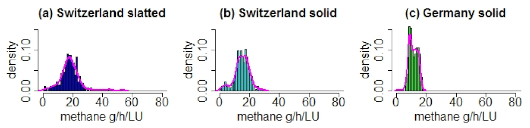
As enteric CH${}_4$ emissions are strongly influenced by dry matter intake, feed composition and thus metabolic processes in rumen, we compared feeding-related values and energy corrected milk at the two farms for the three seasons considered in this study. An overview is provided in

Table 1. Milk yield and feed composition for each site (i.e., S = Switzerland, G = Germany) and the different seasons (i.e., Wi = winter, Sp = spring, Su = summer and Au = autumn).

Site	S	S	S	G	G	G
Season	Wi	Au	Su	Wi	Sp	Su
Energy-corrected
milk per cow (kg day${}^{-1}$)	32.4	33.8	27.7	37.3	37.4	37.0
Dry matter
intake per cow (kg day${}^{-1}$)	21.1	21.6	20.9	26.6	26.0	26.7
Percentage of concentrate
(% of dry matter)	20.4	17.2	20.0	42.3	42.1	42.3
Crude protein
(g kg${}^{-1}$ of dry matter)	168	168	163	173	166	167
Neutral detergent fiber
(g kg${}^{-1}$ of dry matter)	362	360	445	292	338	346
Netto energy lactation
(MJ kg${}^{-1}$ of dry matter)	6.6	6.6	6.3	7.2	7.2	7.1

. Energy corrected milk per cow, dry matter intake, percentage of concentrate, crude protein content and net energy lactation were in general higher in the German farm, while the content of neutral detergent fiber was much higher in the Swiss diet. In general, the reported fluctuations over the seasons were slightly larger in the Swiss farm.

3.1.2. CH${}_4$ Emissions

The average of the CH${}_4$ emission value was highest in the housing compartment with slatted floors in Switzerland and lowest in the housing with solid floors in Germany (see

Table 2. Statistical moments associated with the probability density distributions of CH${}_4$ emission (ME) in g h${}^{-1}$ LU${}^{-1}$, ambient air temperature (T) in ${}^{\circ }$C and the magnitude of the approaching wind (WS) in m s${}^{-1}$ for three naturally ventilated dairy housings. The same number of days per season was considered in all three cases. Due to some missing values, the total number of values in the hourly data sets varied between 265 (Swiss Slatted Floor), 264 (Swiss Solid Floor) and 275 (German Solid Floor). Here, SD refers to the standard deviation of the distribution and CV refers to the coefficient of variation, i.e., the ratio of standard deviation to the mean.

Parameter	Site	Floor Type	Mean	SD	CV	Skewness	Kurtosis
ME	Switzerland	Slatted	18.23	6.79	0.37	1.13	7.68
ME	Switzerland	Solid	14.95	4.96	0.33	−0.50	3.68
ME	Germany	Solid	11.44	2.84	0.25	−0.11	2.68
T	Switzerland	Slatted	13.93	8.05	0.58	−0.08	2.05
T	Switzerland	Solid	14.31	8.02	0.56	−0.13	2.07
T	Germany	Solid	12.55	6.34	0.51	0.23	2.19
WS	Switzerland	Slatted	3.05	2.63	0.86	1.49	5.56
WS	Switzerland	Solid	3.01	2.41	0.80	1.27	4.53
WS	Germany	Solid	1.80	1.28	0.71	0.65	2.54

and Figure 1). The compartment with slatted floors had on average about 22% higher emissions than the compartment with a solid floor at the same location. On the other hand, the two housings with solid floor differed even more, where the compartment in Switzerland had on average about 31% higher CH${}_4$ emissions. A similar trend was observed for the standard deviation of the CH${}_4$ emission values: The value for the slatted floor compartment was about 37% higher than for the solid floor compartment in Switzerland, but the value for the solid floor compartment in Switzerland was again about 75% higher than the value for the solid floor housing in Germany. Focusing on the absolute values of skewness, we see an analog trend: The absolute value for the slatted floor housing was about 126% more than the one for solid floor housing in Switzerland, but the absolute value for the solid floor system in Switzerland was 355% more than for the solid floor system in Germany. For the kurtosis, we observed a slightly different trend where the slatted floor compartment in Switzerland had a value that was 109% more than that of the solid floor compartment in the same location, while the value for the solid floor housing in Switzerland was only 37% higher than for the solid floor housing in Germany. The higher-order moments, skewness and kurtosis, particularly highlighted the differences between slatted and solid floor systems: all three distributions were little to moderately skewed. However, the slatted floor compartment showed a distribution of CH${}_4$ emission values that was right-skewed (i.e., the mean was higher than the peak values), while the solid floor systems showed left-skewed distributions. This means higher emission values were more frequent in the slatted floor system than in the solid floor systems. Moreover, the tail of the distribution was much broader for the slatted floor system compared to the solid floor systems as indicated by a kurtosis that was nearly twice as high. This means that extreme emission values were more likely in the slatted floor system than in the solid floor systems.

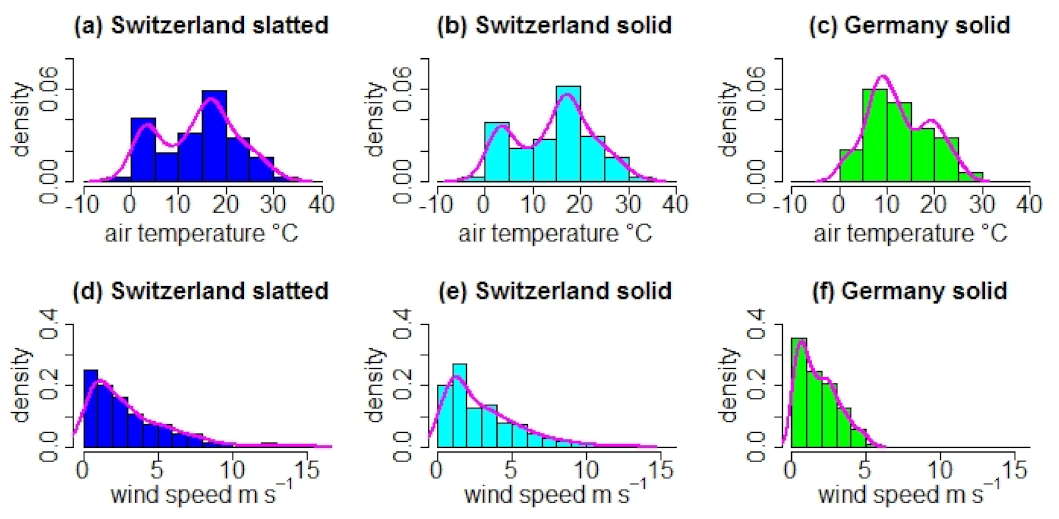
3.1.3. Environmental Conditions

The distributions of temperature and wind speed were more similar among the two locations than the distributions of the emission values (see Figure 2 in comparison to Figure 1). The mean and the standard deviation of the temperature distribution were slightly higher in the Swiss data set (i.e., about 11% and 14%, respectively, for the mean and about 26% for the standard deviation, see Table 2). Moreover, the temperature in the Swiss data set was little left-skewed, while the temperature in the German data set was little more right-skewed. Kurtosis of the temperature distribution was nearly the same for all locations. Kurtosis was, however, far from vanishing, indicating some non-normality also in the temperature distribution.

Furthermore, the mean and standard deviation of the wind speed were considerably larger in the Swiss data set (i.e., about 69% and 67%, respectively, for the mean and about 105% and 88%, respectively, for the standard deviation, see Table 2). The wind speed distribution was in all cases right-skewed, but the skewness was much higher in the Swiss data set (with about 129% and 80%, respectively, higher values of the skewness compared to the German dataset). Furthermore, the kurtosis of the wind speed distribution was about twice as high in the Swiss data set compared to the German one.

The relation between air temperature and wind speed characterizes the convection regime. A rough classification can be obtained using the Richardson number Ri, which indicated that in all three data sets, mixed convection was the dominating regime. In the Swiss data sets, however, forced convection driven by the strong winds was about twice as frequent as in the German data set. On the other hand, natural convection conditions characterized by high temperature gradients and low wind speeds occurred about twice as often in the German data set.

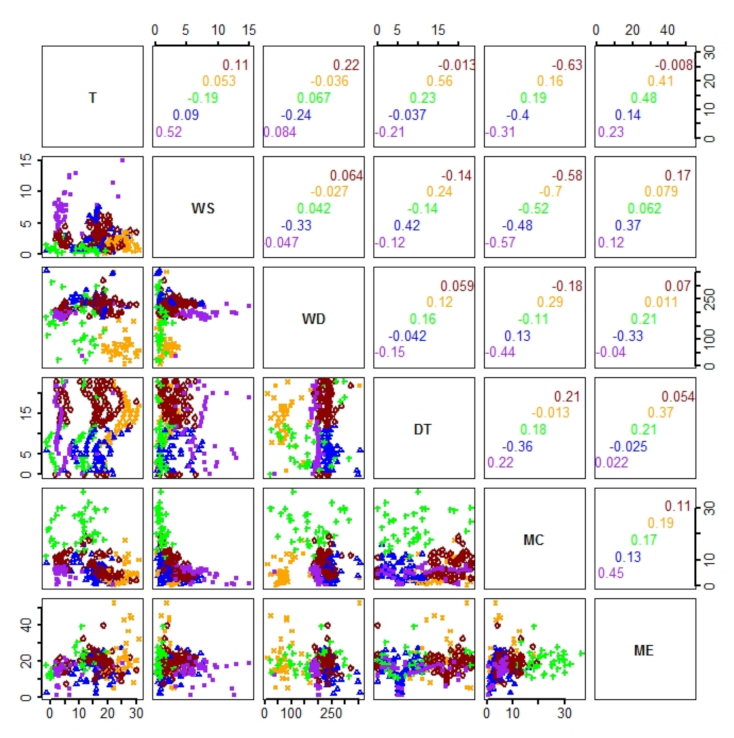
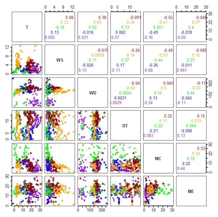
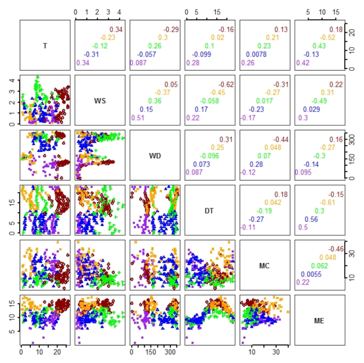
3.2. Pairwise Statistical Relations

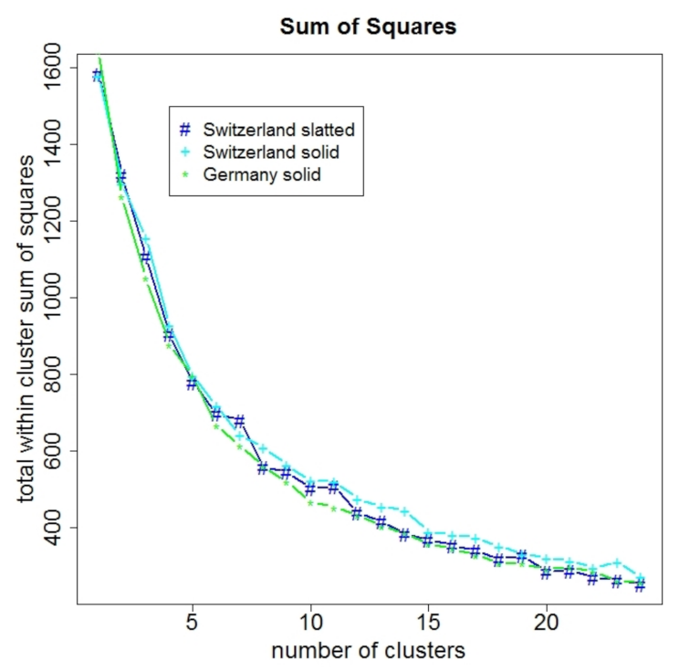
Next, we investigated the statistical dependency between the CH${}_4$ emission value or CH${}_4$ concentration versus air temperature or wind speed (for the entire dataset and for the subsets in

Table 3. Frequency of observed convection regimes for three naturally ventilated dairy housings.

Site	Floor Type	Forced Convection	Mixed Convection	Natural Convection
Switzerland	Slatted	0.40	0.50	0.10
Switzerland	Solid	0.42	0.49	0.09
Germany	Solid	0.21	0.57	0.22

which are associated with the different convection regimes). Since, as described in the previous section, all frequency distributions showed some non-normality, we focused on rank correlations instead of Pearson’s moment correlation. Kendall’s phrasing of correlation resulted, in general, in lower correlation values than the phrasing of Spearman (cf.

Table 4. Spearman’s rank correlation between air temperature (T), wind speed ($WS$), CH${}_4$ emission ($ME$) and CH${}_4$ concentration ($MC$). For each site (i.e., S = Switzerland, G = Germany) and flooring system, the correlation was calculated based on all data as well as based on subsets associated with the regimes forced, mixed and natural convection. p-values in brackets indicate the exceedance probability of normally distributed random variable sets (see Section 2.4.3).

Site	Floor	Regime	T, ME	T, MC	WS, ME	WS, MC
S	Slatted	All	0.22 (p = 0.51)	−0.41 (p = 0.50)	−0.02 (p = 0.44)	−0.57 (p = 0.50)
	Slatted	Forced	0.28 (p = 0.50)	−0.48 (p = 0.51)	−0.25 (p = 0.50)	0.01 (p = 0.44)
S	Slatted	Mixed	0.14 (p = 0.50)	−0.44 (p = 0.49)	−0.04 (p = 0.45)	−0.33 (p = 0.49)
S	Slatted	Natural	0.24 (p = 0.48)	−0.43 (p = 0.50)	−0.22 (p = 0.47)	−0.06 (p = 0.43)
S	Solid	All	−0.08 (p = 0.48)	−0.49 (p = 0.50)	0.12 (p = 0.50)	−0.39 (p = 0.51)
S	Solid	Forced	0.00 (p = 0.44)	−0.55 (p = 0.48)	−0.01 (p = 0.45)	0.06 (p = 0.45)
S	Solid	Mixed	−0.19 (p = 0.49)	−0.60 (p = 0.49)	0.08 (p = 0.47)	−0.03 (p = 0.43)
S	Solid	Natural	0.32 (p = 0.49)	−0.52 (p = 0.49)	−0.20 (p = 0.47)	−0.13 (p = 0.45)
G	Solid	All	0.24 (p = 0.50)	0.11 (p = 0.50)	0.22 (p = 0.50)	0.09 (p = 0.47)
G	Solid	Forced	0.69 (p = 0.51)	0.39 (p = 0.50)	−0.61 (p = 0.51)	−0.31 (p = 0.49)
G	Solid	Mixed	0.14 (p = 0.50)	0.07 (p = 0.47)	0.02 (p = 0.44)	0.03 (p = 0.44)
G	Solid	Natural	−0.09 (p = 0.45)	−0.04 (p = 0.43)	0.26 (p = 0.50)	0.01 (p = 0.45)

and

Table 5. Kendall’s rank correlation between air temperature (T), wind speed ($WS$), CH${}_4$ emission ($ME$) and CH${}_4$ concentration ($MC$). For each site (i.e., S = Switzerland, G = Germany) and flooring system, the correlation was calculated based on all data, as well as based on subsets associated with the regimes forced, mixed and natural convection. p-values in brackets indicate the exceedance probability of normally distributed random variable sets (see Section 2.4.3).

Site	Floor	Regime	T, ME	T, MC	WS, ME	WS, MC
S	Slatted	All	0.15 (p = 0.51)	−0.27 (p = 0.50)	−0.02 (p = 0.44)	−0.39 (p = 0.50)
S	Slatted	Forced	0.20 (p = 0.49)	−0.33 (p = 0.50)	−0.17 (p = 0.49)	0.01 (p = 0.44)
S	Slatted	Mixed	0.11 (p = 0.50)	−0.28 (p = 0.49)	−0.03 (p = 0.45)	−0.22 (p = 0.49)
S	Slatted	Natural	0.17 (p = 0.48)	−0.32 (p = 0.50)	−0.15 (p = 0.47)	−0.02 (p = 0.43)
S	Solid	All	−0.05 (p = 0.47)	−0.34 (p = 0.50)	0.08 (p = 0.49)	−0.28 (p = 0.51)
S	Solid	Forced	0.00 (p = 0.43)	−0.40 (p = 0.49)	−0.01 (p = 0.45)	0.01 (p = 0.44)
S	Solid	Mixed	−0.11 (p = 0.49)	−0.40 (p = 0.49)	0.05 (p = 0.46)	−0.02 (p = 0.43)
S	Solid	Natural	0.24 (p = 0.48)	−0.37 (p = 0.48)	−0.13 (p = 0.46)	−0.13 (p = 0.45)
G	Solid	All	0.17 (p = 0.50)	0.08 (p = 0.50)	0.15 (p = 0.50)	0.07 (p = 0.48)
G	Solid	Forced	0.51 (p = 0.50)	0.32 (p = 0.49)	−0.41 (p = 0.50)	−0.23 (p = 0.49)
G	Solid	Mixed	0.10 (p = 0.50)	0.06 (p = 0.48)	0.01 (p = 0.44)	0.03 (p = 0.44)
G	Solid	Natural	−0.06 (p = 0.45)	−0.07 (p = 0.45)	0.17 (p = 0.50)	0.02 (p = 0.46)

). However, none of the two tested rank correlations (Spearman’s rho and Kendall’s tau) indicated any statistically significant relation. All p-values were much larger than the significance level of $0.05$. The largest absolute values among the correlation coefficients were obtained for the relation between temperature and CH${}_4$ emission under forced convection in the German housing ($\rho =0.69$), the relation between wind speed and CH${}_4$ emission under forced convection in the German housing ($\rho =0.61$), the relation between temperature and CH${}_4$ concentration under mixed convection in the Swiss housing with solid floor ($\rho =-0.60$) and for the relation between wind speed and CH${}_4$ concentration in the slatted floor housing at the Swiss farm considering all convection regimes ($\rho =-0.57$). In contrast to the behavior of the frequency distributions, the rank correlations involving the CH${}_4$ emissions showed no clear trend, which could be associated with the flooring system or the housing location.

In contrast to the rank correlations, mutual information, which evaluates statistical dependency in a broader sense, indicated in most cases a highly significant dependency, i.e., at a significance level of $0.01$, when the data were not split into convection regimes (see

Table 6. Mutual information between air temperature (T), wind speed ($WS$), CH${}_4$ emission ($ME$) and CH${}_4$ concentration ($MC$). For each site and flooring system, the statistical association was calculated based on all data as well as based on subsets associated with forced, mixed and natural convection. p-values indicate the exceedance probability of normally distributed random variable sets (see Section 2.4.3).

Site	Floor	Regime	T, ME	T, MC	WS, ME	WS, MC
S	Slatted	All	0.18 (p < 0.01)	0.22 (p < 0.01)	0.12 (p = 0.06)	0.31 (p < 0.01)
S	Slatted	Forced	0.21 (p < 0.01)	0.30 (p < 0.01)	0.14 (p = 0.01)	0.1 (p = 0.22)
S	Slatted	Mixed	0.20 (p < 0.01)	0.32 (p < 0.01)	0.11 (p = 0.65)	0.25 (p < 0.01)
S	Slatted	Natural	0.17 (p = 0.24)	0.23 (p = 0.08)	0.21 (p = 0.15)	0.09 (p = 0.98)
S	Solid	All	0.15 (p < 0.01)	0.25 (p < 0.01)	0.09 (p = 0.47)	0.27 (p < 0.01)
S	Solid	Forced	0.10 (p = 0.18)	0.27 (p < 0.01)	0.09 (p = 0.29)	0.14 (p = 0.01)
S	Solid	Mixed	0.17 (p = 0.04)	0.39 (p < 0.01)	0.13 (p = 0.37)	0.18 (p = 0.02)
S	Solid	Natural	0.03 (p = 0.68)	0.42 (p < 0.01)	0.03 (p = 0.70)	0.03 (p = 0.67)
G	Solid	All	0.26 (p < 0.01)	0.20 (p < 0.01)	0.14 (p < 0.01)	0.20 (p < 0.01)
G	Solid	Forced	0.50 (p < 0.01)	0.17 (p = 0.08)	0.38 (p < 0.01)	0.14 (p = 0.20)
G	Solid	Mixed	0.21 (p < 0.01)	0.12 (p = 0.06)	0.12 (p = 0.06)	0.15 (p < 0.01)
G	Solid	Natural	0.21 (p = 0.03)	0.24 (p = 0.01)	0.25 (p = 0.01)	0.21 (p = 0.03)

). Only the relation between wind speed and CH${}_4$ emission did not reach the significance level of $0.05$. When looking at the individual convection regimes, the significance of the statistical dependency decreased (particularly in the case of natural convection). The statistical association between CH${}_4$ emission and air temperature and wind speed was in general larger in the German data set than in the two from Switzerland. In total, the relation between wind speed and emission appeared to be the least significant. For the association of temperature and wind speed with the CH${}_4$ concentration, there was no clear trend.

3.3. Clustering

The variation of the sum of squares within the cluster depending on the number of clusters was very similar for all three data sets, as can be seen in Figure 3. The curve did not reveal a clear break point, but around a number of five clusters the curves started to flatten (i.e., the value of the sum of squares within the clusters was only slightly reduced when adding more clusters).

Since the interpretation of individual clusters becomes more challenging with increasing number of clusters, we decided to stay with five clusters for further analysis. We numbered the clusters according to the median emission value within the individual clusters (from 1 for the lowest emission to 5 for the highest emission, see

Table 7. Median values of air temperature (T) in ${}^{\circ }$C, wind speed (WS) in m s${}^{-1}$, wind direction (WD) in ${}^{\circ }$, daytime (DT) in h, CH${}_4$ concentration (MC) in ppm and CH${}_4$ emission (ME) in g h${}^{-1}$ LU${}^{-1}$ within the individual clusters. The median values were extracted from the normalized and sinus-transformed values in the case of wind direction and daytime and then transformed back. For the wind direction, the associated wind corridor is mentioned in brackets.

Site	Floor	Cluster Number	T	WS	WD	DT	MC	ME
S	Slatted	1	3.6	7.1	195.6 (S)	12	5.5	16.1
S	Slatted	2	16.1	1.6	234.9 (SW)	4	4.1	16.1
S	Slatted	3	11.2	0.8	166.7 (S)	10	21.7	18.6
S	Slatted	4	25.2	1.6	58.8 (NO)	14	4.5	19.4
S	Slatted	5	16.0	2.8	231.5 (SW)	15	6.4	19.6
S	Solid	1	24.2	1.5	48.4 (NO)	23	4.1	12.5
S	Solid	2	17.0	1.3	229.6 (SW)	4	5.9	14.7
S	Solid	3	7.7	1.0	198.6 (S)	10	19.1	15.2
S	Solid	4	4.6	6.0	200.6 (S)	1	5.9	15.8
S	Solid	5	16.90	3.3	234.8 (SW)	21	6.7	18.4
G	Solid	1	17.1	0.4	111.1 (O)	3	20.1	9.1
G	Solid	2	10.8	1.1	312.7 (NW)	4	14.0	9.3
G	Solid	3	9.0	2.6	218.9 (SW)	0	8.3	10.6
G	Solid	4	5.3	0.9	5.7 (N)	21	23.1	14.0
G	Solid	5	22.0	2.3	1.8 (N)	15	11.5	14.7

) and show color-coded scatter plots in the lower triangle of Figure 4, Figure 5 and Figure 6 accordingly.

In Figure 4, we show the results from the Swiss data set with slatted floor, and in Figure 5, the results from the Swiss data set with solid floor. Although the clusters were not well separated, we found distinct patterns. There was only a weak diurnal cycle in these data sets, which is mainly associated with the diurnal cycle of air temperature. While the patterns of CH${}_4$ concentration were rather similar for both data sets, the pattern for CH${}_4$ emission differed considerably (particularly in relation to air temperature and wind speed). Very low CH${}_4$ concentrations and emissions are visible during the two milking times due to the absence of the animals in the compartment.

In Figure 6, we show the results from the German data set, which is associated with a solid floor. As in the other two data sets, we observed some overlapping of the clusters but distinct patterns. In contrast to the Swiss data sets, we found a pronounced diurnal cycle in the emission pattern. This was not only associated with the temperature cycle but also with a weak diurnal cycle of wind speed and wind direction.

The calculated pairwise rank correlations within the five clusters varied considerably from cluster to cluster, as shown in the upper triangles of Figure 4, Figure 5 and Figure 6. We noticed that even with clustering, no significant correlation was found.

Taking a closer look at the individual clusters, we found that the five clusters were associated with typical temperature and wind conditions. In general, in each data set we found one cluster associated with high temperatures and low wind speeds. In the data set with slatted floors, this was cluster 4 (i.e., intermediate emission values), while in the data sets with solid floors, it was cluster 1 (i.e., low emission values). Furthermore, we always identified one cluster with high temperatures and moderate wind speeds. This cluster was in all cases associated with cluster 5 (i.e., high emission values). Another cluster was in all cases associated with low temperatures and higher wind speeds. This was cluster 1 in the Swiss data set with slatted floors, cluster 4 in the Swiss data set with solid floors and cluster 3 in the German data set. This means solid floors had rather intermediate emission values and slatted floors had the lowest emissions. Moreover, we found one cluster associated with lower temperatures and lower wind speeds. This was cluster 3 in the Swiss data sets and cluster 4 in the German data set. Again, in all cases, this cluster involved rather intermediate emission values. Finally, the last cluster involved low to intermediate wind speeds and a rather wide temperature range in all data sets. This group involves cluster 2 for all the data sets. This means all cases had rather low emission values.

4. Discussion

4.1. Differences in CH${}_4$ Emissions between Farm Locations

The means of CH${}_4$ emissions for both locations as well as for the two floor systems are within the range of literature values of comparable investigations and a meta-analysis [12,14,45]. However, the average CH${}_4$ emissions for the compartment with the solid floor at the Swiss farm are around 30% higher compared to the German farm (see Table 2).

A substantial part of this deviation can be associated with different feeding strategies. According to the models, around 80% of the CH${}_4$ emissions in dairy housings originate from enteric fermentation [14]. CH${}_4$ is produced in the final phase of the fermentation process of plant cell walls in the rumen [46]. By increasing the amount of concentrate in the diet, the ruminal microbial efficiency and in consequence CH${}_4$ per unit of gross energy intake decrease [47]. When considering the differences in the diets of the two locations, it is noticeable that the proportion of concentrates in dry matter of the German farm is more than twice as high compared to the Swiss farm (see Table 1). Analogously, the amount of neutral detergent fiber in the diet was higher on the Swiss farm. Numerous investigations and models describe that a higher proportion of concentrate in the diet leads to a reduction in CH${}_4$ emissions per cow [46,47,48,49,50].

The remaining part of the deviation between the two farm locations may be attributed to uncertainties of any or both measurement approaches (i.e., artificial versus natural tracer ratio method). For example, Qu et al. concluded from a meta-analysis that measurement methods could have a significant impact on the CH${}_4$ emission estimates [51]. Moreover, Edouard et al. reported that CO${}_2$ balancing led in general to about 10% lower ventilation rate estimates compared to the artificial tracer method [52]. Finally, there are uncertainties related to the slightly different sampling strategies to determine indoor methane concentration.

4.2. Effect of Floor Type and Climate Parameters on CH${}_4$ Emissions

While excrement-based CH${}_4$ emissions have a minor contribution in solid floor systems, in our study, the slurry storage underneath the slats seems to be an important source of CH${}_4$ emissions. Within the Swiss dairy housing, the averaged CH${}_4$ emissions from the compartment with slatted floors were more than 20% higher compared to those from the compartment with solid floors (see Table 1). In contrast to our findings, in a meta-analysis, Poteko et al. found no significant difference in CH${}_4$ emissions between solid and perforated floors [12]. With regard to mitigation measures, Monteny et al., however, indicated slurry storage inside the housing as a relevant CH${}_4$ emission source [16]. Furthermore, a significant temperature effect on CH${}_4$ emissions is reported in the literature [12,53]. Following the Arrhenius law, the CH${}_4$ emissions from the slatted floor system with slurry storage in the housing are expected to increase exponentially with increasing ambient temperature. A notable increase in slurry-based CH${}_4$ emissions has been reported for temperatures above about 15 ${}^{\circ }$C [26]. Since the temperature distribution in the three data sets is rather symmetric and the average is only slightly below 15 ${}^{\circ }$C, the higher emissions from the slatted floor system compared to the solid floor systems must be expected. Moreover, if the wind speed near the active emission surface increases, the thickness of the boundary layer between slurry and atmosphere and in consequence the resistance of diffusive gas transfer from the manure to the atmosphere decreases, which leads to higher local emission rates for slurry-based CH${}_4$ [23]. If the active emission surface is larger, as in the slatted floor system with slurry storage inside the housing compared to the solid floor system, the wind effect is larger. This is also in line with the observed differences in the average emission values of the slatted and solid floor systems.

4.3. Statistical Association and Clustering

While there was no significant rank correlation between the environmental variables (i.e., air temperature and wind speed) and the CH${}_4$ concentration or emission, we found that there was still a significant share of information indicating a statistical dependency. There was, however, no clear prevalence for a floor system regarding the strength of the statistical relation between environmental variables and CH${}_4$ concentration or emission. This might be related to the dominant influence of enteric CH${}_4$ emissions in comparison to the slurry-based emissions [14,15]. The absence of significant rank correlations in the presence of significant mutual information is a strong indication for a nonlinear and even non-monotonic relation. It is further an indication for an indirect relation mediated probably by multiple behavioral, physiological and microbiological responses to the environmental changes. This is inline with recent findings that microclimatic conditions and housing management induce variations in daily CH${}_4$ emission patterns [54]. Moreover, there is likely an effect of nonlinear changes in the airflow pattern related to the switching between convection regimes since the airflow pattern affects the representativity of individual gas sampling locations and in consequence the accuracy of the derived concentration and emission values. We found that in our data sets, the significance of the mutual information was particularly low under natural convection. This might be related to the fact that gas sampling setups are typically optimized for the flow pattern under the dominating mixed convection, from which the pattern under natural convection strongly deviates. In consequence, larger inaccuracies in the measured concentration/emission values can be expected under natural convection (cf., e.g., [55]). In addition to the low significance of mutual information under natural convection, we found no clear trend among the different convection regimes. This might be related to the very rough definition of the convection switching points. In particular, the wind speed values, which were used for the calculation of the Richardson number in this study, were not directly taken from the inlet of the housing. Moreover, we partly observed a loss of significance in the “natural”, “forced” and “mixed” subsets compared with the data sets with all convection regimes, which indicates that the number of data points in the convection regime-related subsets might be too small to draw general conclusions.

Nevertheless, the clustering highlighted a relation between air temperature, wind speed (i.e., the convection type) and the typical CH${}_4$ emission strength.

For example, the cluster with the highest CH${}_4$ emissions was associated with the highest temperatures (i.e., low-temperature gradients between cows and ambient air) as well as moderate wind speeds. This is in line with state-of-the-art knowledge that high temperatures boost the CH${}_4$ emission release from active emission surfaces. In addition, the induced forced convection in the framework of such environmental conditions promotes airflow patterns that can efficiently remove pollutant air. This is further supported by the fact that within this cluster, we mainly found wind directions that nearly induce a cross-flow. In the German data set, the prevailing wind direction from the north also means a potential additional entry of CH${}_4$ from the nearby milking parlor and other dairy buildings.

In contrast, in the cluster where the temperature is low but the wind speed is still high, a situation of mixed convection must be assumed. This cluster was also rather associated with wind direction, indicating cross-flow conditions. These two aspects typically result in rather homogeneous flow patterns without pronounced zones of gas trapping. In addition, pollutant air can be removed here effectively. However, this cluster led to considerably lower emission values, particularly in the data set with the slatted floor. This can be well explained by the fact that the slurry-based CH${}_4$ release is very low at the low temperatures, while with an average temperature between 5 and 10${}^{\circ }$, no significant increase in the enteric CH${}_4$ release can be expected.

On the other hand, the other three clusters that were associated with rather low wind speeds would in a first approximation be expected to result in very low emissions. This was, however, not true for all the clusters. For example, the case with high temperature and low wind speed was associated with the lowest emissions for the solid floor systems but not for the slatted floor system. Here, the strong effect of exponential increase in slurry-based emissions with raising temperatures probably overcompensated for the effect of gas trapping due to low wind speeds and wind directions far from cross-flow conditions. Another example is the case with low temperature and low wind speed, which resulted on average in rather high CH${}_4$ emissions. The related temperature range does not imply a strong increase in CH${}_4$ emissions from enteric fermentation, so the higher emissions cannot be explained by stronger local CH${}_4$ release. However, the combination of low temperature and low wind speed indicates a shift towards natural convection, which is associated with completely different airflow patterns.

5. Conclusions

We confirmed our main hypothesis that slatted and solid floor systems show different CH${}_4$ emission patterns. As expected, the average emission from the slatted floor system was the highest. The difference between the two farm locations with solid floors was, however, about 7% higher than the difference between the two floor systems in the Swiss farm. This is an indication of the effect of enteric CH${}_4$, which plays a significant role in the CH${}_4$ emission level. We further found that the frequency distributions of the emission values in all three data sets were highly non-normal, indicating that Pearson correlation analysis might be misleading. The mean and the standard deviation of the emission distribution were mainly influenced by the location of the barn, while the skewness and kurtosis were more influenced by the flooring system.

While there was an obvious divergence between the geographical locations, we obtained only low values of the rank correlation measures, which evaluate the strength of a linear relationship between two sets of ranks. Moreover, at the given significance level these statistical measures could not distinguish whether or not coincidences between CH${}_4$ concentrations or emission values and air temperature or wind speed were nonrandom. On the other hand, the mutual information, which does not look for monotonic functional relations but for shared information in the time series, indicated highly significant relations for almost all variable pairs except for the case of wind speed versus CH${}_4$ emission.

Our study succeeded in its aim to provide a basis for the selection of the most important environmental variables for future CH${}_4$ emission projections in the following sense: The temperature was highlighted as particularly relevant for both soil types, while wind speed alone did not prove to be decisive. The clustering analysis, however, revealed that in the interplay with temperature there is still a relation between wind speed and emission strength.

Clustering was consistent among the three data sets, indicating the following five typical clusters: (1) high temperature and moderate wind speed with prevalence for high CH${}_4$ emissions, (2) low temperature and high wind speed with intermediate emission strength in the solid floor systems and low CH${}_4$ emission strength for slatted floor, (3) low temperature and low wind speed with intermediate CH${}_4$ emission strength, (4) high temperature and low wind speed with low CH${}_4$ emission strength in the solid floor systems but intermediate CH${}_4$ emission strength in the slatted floor systems as well as (5) moderate temperatures and low wind speeds with prevalence for low CH${}_4$ emissions. The first two mentioned clusters can be easily explained by the effect of high temperatures and increased diffusion at high wind speeds, which amplify the slurry-based emissions. The behavior in the last two clusters is more complex and likely a result of the competing, contradicting influences of high temperature and high diffusive resistance at low wind speeds. The behavior of the third mentioned cluster, finally, seems to be rather related to the airflow pattern in the barn that emerges from specific combinations of temperature and wind speed.

Further research with larger data sets capturing a broader range of environmental conditions and inter-farm-variability is advisable to confirm the observed trends. In future work, it will also be valuable to measure and quantify factors related to farm animals in addition to describing the interaction between the biological characteristics of cows on farms and environmental factors.

References

1. WMO. WMO Statement on the State of the Global Climate in 2017; WMO-No.1212; Publications Board World Meteorological Organization (WMO), Ed.; World Meteorological Organization: Geneva, Switzerland, 2018. [Google Scholar]
2. Sutton, M.A.; Bleeker, A.; Howard, C.; Erisman, J.; Abrol, Y.; Bekunda, M.; Datta, A.; Davidson, E.; de Vries, W.; Oenema, O.; et al. Our Nutrient World. The Challenge to Produce More Food & Energy with Less Pollution; Technical Report; Centre for Ecology & Hydrology: Edinburgh, UK, 2013. [Google Scholar]
3. Masson-Delmotte, V.; Zhai, P.; Pörtner, H.O.; Roberts, D.; Skea, J.; Shukla, P.R.; Pirani, A.; Moufouma-Okia, W.; Péan, C.; Pidcock, R.; et al. Global Warming of 1.5 ∘C. An IPCC Special Report on the Impacts of Global Warming of 1.5 ∘C above Pre-Industrial Levels and Related Global Greenhouse Gas Emission Pathways, in the Context of Strengthening the Global Response to the Threat of Climate Change, Sustainable Development, and Efforts to Eradicate Poverty. Technical Report. Intergovernmental Panel on Climate Change (IPCC). 2018. Available online: https://www.ipcc.ch/site/assets/uploads/sites/2/2019/06/SR15_Full_Report_High_Res.pdf (accessed on 20 December 2021).
4. Shukla, P.R.; Skea, J.; Calvo Buendia, E.; Masson-Delmotte, V.; Pörtner, H.O.; Roberts, D.C.; Zhai, P.; Slade, R.; Connors, S.; van Diemen, R.; et al. Climate Change and Land: An IPCC Special Report on Climate Change, Desertification, Land Degradation, Sustainable Land Management, Food Security, and Greenhouse Gas Fluxes in Terrestrial Ecosystems. Technical Report. Intergovernmental Panel on Climate Change (IPCC). 2019. Available online: https://www.ipcc.ch/site/assets/uploads/sites/4/2020/02/SRCCL-Complete-BOOK-LRES.pdf (accessed on 20 December 2021).
5. Food and Agriculture Organization of the United Nations (FAO). The Future of Food and Agriculture—Trends and Challenges; Technical Report; FAO: Rome, Italy, 2017; 180p, Available online: http://www.fao.org/3/a-i6583e.pdf (accessed on 20 December 2021)ISBN 978-92-5-109551-5.
6. Food and Agriculture Organization of the United Nations (FAO). World Livestock: Transforming the Livestock Sector through the Sustainable Development Goals—Full Report; Technical Report; FAO: Rome, Italy, 2018; 222p, Available online: http://www.fao.org/3/CA1201EN/ca1201en.pdf (accessed on 20 December 2021).
7. Gerber, P.J.; Steinfeld, H.; Henderson, B.; Mottet, A.; Opio, C.; Dijkman, J.; Falcucci, A.; Tempio, G. Tackling Climate Change through Livestock—A Global Assessment of Emissions and Mitigation Opportunities; Technical Report; Food and Agriculture Organization of the United Nations (FAO): Rome, Italy, 2013; 26p, Available online: http://www.fao.org/3/i3437e/i3437e.pdf (accessed on 20 December 2021).
8. Saunois, M.; Stavert, A.R.; Poulter, B.; Bousquet, P.; Canadell, J.G.; Jackson, R.B.; Raymond, P.A.; Dlugokencky, E.J.; Houweling, S.; Patra, P.K.; et al. The global methane budget 2000–2017. Earth Syst. Sci. Data 2020, 12, 1561–1623. [Google Scholar] [CrossRef]
9. Bewley, J.; Robertson, L.; Eckelkamp, E. A 100-Year Review: Lactating dairy cattle housing management. J. Dairy Sci. 2017, 100, 10418–10431. [Google Scholar] [CrossRef] [PubMed]
10. Galama, P.; Ouweltjes, W.; Endres, M.; Sprecher, J.; Leso, L.; Kuipers, A.; Klopčič, M. Symposium review: Future of housing for dairy cattle. J. Dairy Sci. 2020, 103, 5759–5772. [Google Scholar] [CrossRef] [PubMed]
11. Hempel, S.; Menz, C.; Pinto, S.; Galán, E.; Janke, D.; Estellés, F.; Müschner-Siemens, T.; Wang, X.; Heinicke, J.; Zhang, G.; et al. Heat stress risk in European dairy cattle husbandry under different climate change scenarios—Uncertainties and potential impacts. Earth Syst. Dyn. 2019, 10, 859–884. [Google Scholar] [CrossRef] [Green Version]
12. Poteko, J.; Zähner, M.; Schrade, S. Effects of housing system, floor type and temperature on ammonia and methane emissions from dairy farming: A meta-analysis. Biosyst. Eng. 2019, 182, 16–28. [Google Scholar] [CrossRef]
13. Schrade, S.; Zeyer, K.; Gygax, L.; Emmenegger, L.; Hartung, E.; Keck, M. Ammonia emissions and emission factors of naturally ventilated dairy housing with solid floors and an outdoor exercise area in Switzerland. Atmos. Environ. 2012, 47, 183–194. [Google Scholar] [CrossRef]
14. Ngwabie, N.M.; Vanderzaag, A.; Jayasundara, S.; Wagner-Riddle, C. Measurements of emission factors from a naturally ventilated commercial barn for dairy cows in a cold climate. Biosyst. Eng. 2014, 127, 103–114. [Google Scholar] [CrossRef]
15. Monteny, G.; Groenestein, C.; Hilhorst, M. Interactions and coupling between emissions of methane and nitrous oxide from animal husbandry. Nutr. Cycl. Agroecosyst. 2001, 60, 123–132. [Google Scholar] [CrossRef]
16. Monteny, G.J.; Bannink, A.; Chadwick, D. Greenhouse gas abatement strategies for animal husbandry. Agric. Ecosyst. Environ. 2006, 112, 163–170. [Google Scholar] [CrossRef]
17. Beauchemin, K.; McGinn, S.; Benchaar, C.; Holtshausen, L. Crushed sunflower, flax, or canola seeds in lactating dairy cow diets: Effects on methane production, rumen fermentation, and milk production. J. Dairy Sci. 2009, 92, 2118–2127. [Google Scholar] [CrossRef]
18. Ngwabie, N.; Jeppsson, K.H.; Gustafsson, G.; Nimmermark, S. Effects of animal activity and air temperature on methane and ammonia emissions from a naturally ventilated building for dairy cows. Atmos. Environ. 2011, 45, 6760–6768. [Google Scholar] [CrossRef]
19. Saha, C.; Ammon, C.; Berg, W.; Fiedler, M.; Loebsin, C.; Sanftleben, P.; Brunsch, R.; Amon, T. Seasonal and diel variations of ammonia and methane emissions from a naturally ventilated dairy building and the associated factors influencing emissions. Sci. Total Environ. 2014, 468, 53–62. [Google Scholar] [CrossRef] [PubMed]
20. Hempel, S.; Saha, C.K.; Fiedler, M.; Berg, W.; Hansen, C.; Amon, B.; Amon, T. Non-linear temperature dependency of ammonia and methane emissions from a naturally ventilated dairy barn. Biosyst. Eng. 2016, 145, 10–21. [Google Scholar] [CrossRef] [Green Version]
21. Yadav, B.; Singh, G.; Wankar, A.; Dutta, N.; Chaturvedi, V.; Verma, M.R. Effect of simulated heat stress on digestibility, methane emission and metabolic adaptability in crossbred cattle. Asian-Australas. J. Anim. Sci. 2016, 29, 1585. [Google Scholar] [CrossRef]
22. Hempel, S.; Willink, D.; Janke, D.; Ammon, C.; Amon, B.; Amon, T. Methane emission characteristics of naturally ventilated cattle buildings. Sustainability 2020, 12, 4314. [Google Scholar] [CrossRef]
23. Husted, S. An open chamber technique for determination of methane emission from stored livestock manure. Atmos. Environ. Part A. Gen. Top. 1993, 27, 1635–1642. [Google Scholar] [CrossRef]
24. Im, S.; Petersen, S.O.; Lee, D.; Kim, D.H. Effects of storage temperature on CH4 emissions from cattle manure and subsequent biogas production potential. Waste Manag. 2020, 101, 35–43. [Google Scholar] [CrossRef]
25. Schmithausen, A.J.; Schiefler, I.; Trimborn, M.; Gerlach, K.; Südekum, K.H.; Pries, M.; Büscher, W. Quantification of methane and ammonia emissions in a naturally ventilated barn by using defined criteria to calculate emission rates. Animals 2018, 8, 75. [Google Scholar] [CrossRef] [Green Version]
26. Amon, B.; Kryvoruchko, V.; Fröhlich, M.; Amon, T.; Pöllinger, A.; Mösenbacher, I.; Hausleitner, A. Ammonia and greenhouse gas emissions from a straw flow system for fattening pigs: Housing and manure storage. Livest. Sci. 2007, 112, 199–207. [Google Scholar] [CrossRef]
27. Cárdenas, A.; Ammon, C.; Schumacher, B.; Stinner, W.; Herrmann, C.; Schneider, M.; Weinrich, S.; Fischer, P.; Amon, T.; Amon, B. Methane emissions from the storage of liquid dairy manure: Influences of season, temperature and storage duration. Waste Manag. 2021, 121, 393–402. [Google Scholar] [CrossRef]
28. Kori, R.K.; Hasan, W.; Jain, A.K.; Yadav, R.S. Cholinesterase inhibition and its association with hematological, biochemical and oxidative stress markers in chronic pesticide exposed agriculture workers. J. Biochem. Mol. Toxicol. 2019, 33, e22367. [Google Scholar] [CrossRef]
29. Zetouni, L.; Kargo, M.; Norberg, E.; Lassen, J. Genetic correlations between methane production and fertility, health, and body type traits in Danish Holstein cows. J. Dairy Sci. 2018, 101, 2273–2280. [Google Scholar] [CrossRef]
30. Van Gastelen, S.; Mollenhorst, H.; Antunes-Fernandes, E.; Hettinga, K.; van Burgsteden, G.; Dijkstra, J.; Rademaker, J. Predicting enteric methane emission of dairy cows with milk Fourier-transform infrared spectra and gas chromatography–based milk fatty acid profiles. J. Dairy Sci. 2018, 101, 5582–5598. [Google Scholar] [CrossRef] [Green Version]
31. Ellis, J.; Kebreab, E.; Odongo, N.; McBride, B.; Okine, E.; France, J. Prediction of methane production from dairy and beef cattle. J. Dairy Sci. 2007, 90, 3456–3466. [Google Scholar] [CrossRef]
32. Hempel, S.; Adolphs, J.; Landwehr, N.; Willink, D.; Janke, D.; Amon, T. Supervised Machine Learning to Assess Methane Emissions of a Dairy Building with Natural Ventilation. Appl. Sci. 2020, 10, 6938. [Google Scholar] [CrossRef]
33. Bolboaca, S.D.; Jäntschi, L. Pearson versus Spearman, Kendall’s tau correlation analysis on structure-activity relationships of biologic active compounds. Leonardo J. Sci. 2006, 5, 179–200. [Google Scholar]
34. Spearman, C. Footrule for measuring correlation. Br. J. Psychol. 1906, 2, 89. [Google Scholar] [CrossRef]
35. Kendall, M.G. A new measure of rank correlation. Biometrika 1938, 30, 81–93. [Google Scholar] [CrossRef]
36. Duncan, T.E. On the calculation of mutual information. SIAM J. Appl. Math. 1970, 19, 215–220. [Google Scholar] [CrossRef] [Green Version]
37. Gierlichs, B.; Batina, L.; Tuyls, P.; Preneel, B. Mutual information analysis. In Proceedings of the International Workshop on Cryptographic Hardware and Embedded Systems, Washington, DC, USA, 10–13 August 2008; Springer: Berlin/Heidelberg, Germany, 2008; pp. 426–442. [Google Scholar]
38. Jain, A.K. Data clustering: 50 years beyond k-means. In Proceedings of the Joint European Conference on Machine Learning and Knowledge Discovery in Databases, Antwerp, Belgium, 15–18 September 2008; Springer: Berlin/Heidelberg, Germany, 2008; pp. 3–4. [Google Scholar]
39. Mohn, J.; Zeyer, K.; Keck, M.; Keller, M.; Zähner, M.; Poteko, J.; Emmenegger, L.; Schrade, S. A dual tracer ratio method for comparative emission measurements in an experimental dairy housing. Atmos. Environ. 2018, 179, 12–22. [Google Scholar] [CrossRef]
40. Poteko, J.; Zähner, M.; Steiner, B.; Schrade, S. Residual soiling mass after dung removal in dairy loose housings: Effect of scraping tool, floor type, dung removal frequency and season. Biosyst. Eng. 2018, 170, 117–129. [Google Scholar] [CrossRef]
41. Leinweber, T.; Zähner, M.; Schrade, S. Evaluation of a dung-removal robot for use in dairy housing from an ethological and process-engineering point of view. Landtechnik 2019, 74, 55–68. [Google Scholar]
42. Pedersen, S.; Sällvik, K. Climatization of Animal Houses. Heat and Moisture Production at Animal and House Levels; Danish Insitute of Agricultural Sciences: Horsens, Denmark, 2002; pp. 1–46. [Google Scholar]
43. Willink, D.; Hempel, S.; Janke, D.; Amon, B.; Amon, T. High resolution long-term measurements of carbon dioxide, ammonia, and methane concentrations in two naturally ventilated dairy barns. Publisso ZB Med Repos. Life Sci. 2020. [Google Scholar] [CrossRef]
44. Doumbia, E.M.; Janke, D.; Yi, Q.; Prinz, A.; Amon, T.; Kriegel, M.; Hempel, S. A parametric model for local air exchange rate of naturally ventilated barns. Agronomy 2021, 11, 1585. [Google Scholar] [CrossRef]
45. Poteko, J.; Schrade, S.; Zeyer, K.; Mohn, J.; Zaehner, M.; Zeitz, J.O.; Kreuzer, M.; Schwarm, A. Methane emissions and milk fatty acid profiles in dairy cows fed linseed, measured at the group level in a naturally ventilated housing and individually in respiration chambers. Animals 2020, 10, 1091. [Google Scholar] [CrossRef]
46. Aguerre, M.J.; Wattiaux, M.A.; Powell, J.; Broderick, G.A.; Arndt, C. Effect of forage-to-concentrate ratio in dairy cow diets on emission of methane, carbon dioxide, and ammonia, lactation performance, and manure excretion. J. Dairy Sci. 2011, 94, 3081–3093. [Google Scholar] [CrossRef]
47. Benchaar, C.; Pomar, C.; Chiquette, J. Evaluation of dietary strategies to reduce methane production in ruminants: A modelling approach. Can. J. Anim. Sci. 2001, 81, 563–574. [Google Scholar] [CrossRef]
48. Knapp, J.R.; Laur, G.; Vadas, P.A.; Weiss, W.P.; Tricarico, J.M. Invited review: Enteric methane in dairy cattle production: Quantifying the opportunities and impact of reducing emissions. J. Dairy Sci. 2014, 97, 3231–3261. [Google Scholar] [CrossRef] [Green Version]
49. Olijhoek, D.; Løvendahl, P.; Lassen, J.; Hellwing, A.; Höglund, J.; Weisbjerg, M.; Noel, S.; McLean, F.; Højberg, O.; Lund, P. Methane production, rumen fermentation, and diet digestibility of Holstein and Jersey dairy cows being divergent in residual feed intake and fed at 2 forage-to-concentrate ratios. J. Dairy Sci. 2018, 101, 9926–9940. [Google Scholar] [CrossRef] [Green Version]
50. van Gastelen, S.; Dijkstra, J.; Bannink, A. Are dietary strategies to mitigate enteric methane emission equally effective across dairy cattle, beef cattle, and sheep? J. Dairy Sci. 2019, 102, 6109–6130. [Google Scholar] [CrossRef] [Green Version]
51. Qu, Q.; Groot, J.C.; Zhang, K.; Schulte, R.P. Effects of housing system, measurement methods and environmental factors on estimating ammonia and methane emission rates in dairy barns: A meta-analysis. Biosyst. Eng. 2021, 205, 64–75. [Google Scholar] [CrossRef]
52. Edouard, N.; Mosquera, J.; van Dooren, H.J.; Mendes, L.B.; Ogink, N.W. Comparison of CO2- and SF6-based tracer gas methods for the estimation of ventilation rates in a naturally ventilated dairy barn. Biosyst. Eng. 2016, 149, 11–23. [Google Scholar] [CrossRef] [Green Version]
53. Pereira, J.; Misselbrook, T.H.; Chadwick, D.R.; Coutinho, J.; Trindade, H. Effects of temperature and dairy cattle excreta characteristics on potential ammonia and greenhouse gas emissions from housing: A laboratory study. Biosyst. Eng. 2012, 112, 138–150. [Google Scholar] [CrossRef]
54. D’Urso, P.R.; Arcidiacono, C.; Cascone, G. Environmental and Animal-Related Parameters and the Emissions of Ammonia and Methane from an Open-Sided Free-Stall Barn in Hot Mediterranean Climate: A Preliminary Study. Agronomy 2021, 11, 1772. [Google Scholar] [CrossRef]
55. Doumbia, E.M.; Janke, D.; Yi, Q.; Zhang, G.; Amon, T.; Kriegel, M.; Hempel, S. On Finding the Right Sampling Line Height through a Parametric Study of Gas Dispersion in a NVB. Appl. Sci. 2021, 11, 4560. [Google Scholar] [CrossRef]
Figure 1. Histograms showing the density distributions of CH 4 emission per livestock unit (LU) in the three datasets: (a) compartment with slatted floor at Swiss farm, (b) compartment with solid floor at Swiss farm, and (c) building with solid floor at German farm. Breaks were set from 0 to 100 in steps of 1 for the binning.
Agronomy 12 00381 g001
Figure 2. Histograms showing the density distributions of air temperature (upper row) and wind speed (lower row) in the three data sets: (a,d) compartment with slatted floor at Swiss farm, (b,e) compartment with solid floor at Swiss farm, and (c,f) building with solid floor at German farm. Breaks were set from −10 to 40 in steps of 5 for the binning of the temperature data and from 0 to 16 in steps of 1 for the binning of the wind data.
Agronomy 12 00381 g002
Figure 3. Clustering of normalized sets of environmental variables and CH 4 concentration and emission. Variation of the total sum of squares within the clusters depending on the number of clusters using the k-means algorithm for all three data sets.
Agronomy 12 00381 g003
Figure 4. Clustering of air temperature (T) in C, wind speed (WS) in m s 1 , wind direction (WD) in , daytime (DT) in h, CH 4 concentration (MC) in ppm and CH 4 emission (ME) in g h 1 LU 1 in the data set of the slatted floor system in Switzerland. The abbreviations on the diagonal indicate which variables are displayed at the axes in the respective row and column of the plot. Cluster affiliation is color-coded in the scatter plots in the lower triangle in violet, blue, green, orange and red (ordered from low median of emission to high median of emission in the cluster). The upper triangle shows the related Spearman’s rank correlation values for the individual clusters in the same color-coding.
Agronomy 12 00381 g004
Figure 5. Clustering of air temperature (T) in C, wind speed (WS) in m s 1 , wind direction (WD) in , daytime (DT) in h, CH 4 concentration (MC) in ppm and CH 4 emission (ME) in g h 1 LU 1 in the data set of the solid floor system in Switzerland. The abbreviations on the diagonal indicate which variables are displayed at the axes in the respective row and column of the plot. Cluster affiliation is color-coded in the scatter plots in the lower triangle in violet, blue, green, orange and red (ordered from low median of emission to high median of emission in the cluster). The upper triangle shows the related Spearman’s rank correlation values for the individual clusters in the same color code.
Agronomy 12 00381 g005
Figure 6. Clustering of air temperature (T) in C, wind speed (WS) in m s 1 , wind direction (WD) in , daytime (DT) in h, CH 4 concentration (MC) in ppm and CH 4 emission (ME) in g h 1 LU 1 in the data set of the solid floor system in Germany. The abbreviations on the diagonal indicate which variables are displayed at the axes in the respective row and column of the plot. Cluster affiliation is color-coded in the scatter plots in the lower triangle in violet, blue, green, orange and red (ordered from low median of emission to high median of emission in the cluster). The upper triangle shows the related Spearman rank correlation values for the individual clusters in the same color code.
Agronomy 12 00381 g006