
Techno-Economic Assessment of an Office-Based Indoor Farming Unit


Biobased Resources in the Bioeconomy (340b), Institute of Crop Science, University of Hohenheim, Fruwirthstr. 23, 70599 Stuttgart, Germany
*
Author to whom correspondence should be addressed.
Agronomy 2022, 12(12), 3182; https://doi.org/10.3390/agronomy12123182
Submission received: 12 October 2022
/
Revised: 25 November 2022
/
Accepted: 13 December 2022
/
Published: 15 December 2022
(This article belongs to the Special Issue Social-Ecologically More Sustainable Agricultural Production)
Abstract
:Decentralized, smart indoor cultivation systems can produce herbs and vegetables for fresh and healthy daily nutrition of the urban population. This study assesses technical and resource requirements, productivity, and economic viability of the “Smart Office Farm” (SOF), based on a 5-week production cycle of curled lettuce, lolo rosso, pak choi and basil at three photosynthetic photon flux density (PPFD) levels using a randomized block design. The total fresh matter yield of consumable biomass of all crops was 2.5 kg m−2 with operating expenses (without labor costs) of EUR 53.14 kg−1; more than twice as expensive compared to large-scale vertical farm and open-field cultivation. However, there is no need to add trade margins and transportation costs. The electricity supply to SOF is 73%, by far the largest contributor to operational costs of office-based crop production. Energetic optimizations such as a more homogeneous PPFD distribution at the plant level, as well as adaptation of light quality and quantity to crop needs can increase the economic viability of such small indoor farms. With reduced production costs, urban indoor growing systems such as SOF can become a viable option for supporting fresh and healthy daily nutrition in urban environments.
1. Introduction
The number of people living on planet earth is expected to rise to 9.7 billion by 2050 [1] and the growing global population will require about 60% more food from 2007 to 2050 [2]. Additionally, urbanization is transforming our society, since more than half of the world’s population now lives in cities. This proportion is expected to increase to 68% by 2050 [3].
These figures shape the agricultural sector and the way we feed our cities. To date, our cities are highly dependent on food imports and linear value chains with food being imported, consumed and waste moved out. However, sustainable cities need to close the open-loop system [4] and to design circular and decentralized value chains.
Urban agriculture is becoming increasingly recognized as a viable option to support global food security in times of climate change, resource constraints and growing food demand. Highly productive, resource-efficient urban cultivation systems can play a key role over the next decade in turning cities sustainable [5,6,7].
As defined by [8] “Most broadly, urban agriculture refers to growing and raising food crops and animals in an urban setting to feed local populations”. It includes indoor and outdoor agriculture and ranges from food grown on the balcony (Bio-Balkon [9], Geco-Gardens [10]), to large production facilities such as AeroFarms in the US [11].
Urban agriculture has multiple environmental, economic and social sustainability benefits to both developing and post-industrial cities [12]. “Furthermore, it contributes to ten key societal challenges of urbanization: climate change, food security, biodiversity and ecosystem services, agricultural intensification, resource efficiency, urban renewal and regeneration, land management, public health, social cohesion, and economic growth” [13].
According to the Worldwatch Institute, globally, about 15–20% of food is produced today in urban and peri-urban areas [13]. For example, urban cultivation accounts for 5–10% of total noncereal crop production, which has a total market volume of USD 1509 billion [6]. In addition to food, urban agriculture provides valuable ecosystem services through the creation of new green areas. These can, for example, reduce heat islands and mitigate storm water impacts, thus increasing cities’ resilience to climate change impacts [14]. Globally, the ecosystem services provided by urban agriculture are worth USD 88 to 164 billion, increasing the well-being of urban inhabitants [6].
Urban agriculture can transform the typical structure of rural food production and urban food consumption towards more decentralized production systems [7] that increase local access to and availability of food, two crucial factors of food security [15]. For improving the supply of fresh fruits and vegetables, in particular, the crops that are deemed suitable for urban production are those consumed as fresh functional foods supporting fresh and healthy daily nutrition [16,17].
As a result of the change from traditional linear supply chains to short, local and circular supply chains based on urban production, a new food distribution infrastructure in urban areas can emerge with lower food miles and high resource recovery. For instance, Pirog and Benjamin [18] show that conventional US broccoli travels 92 times further than local broccoli and average vegetables travel 27 times longer. The food in US supermarkets has travelled on average about 2000 km between the production and consumption site, releasing between 0.8 and 1.9 kg of CO2 Mg−1 km−1. The production of Berlin’s food is 72% from domestic land, 7% in the EU and 21% outside the EU [19,20]. Ackerman et al. [14] found that the decrease in food miles can reduce food waste through a reduction in spoilage during transport and storage, which is another important benefit of decentralized urban food systems. The decrease in food waste directly increases both resource-use and the energy-use efficiency of food production. In fact, resource circulation in cities through urban agriculture is an important enabler for the transition towards a sustainable urban bioeconomy [21].
Decentralized, smart and automated production systems can be important for producing vegetables and herbs at the place of consumption, e.g., at offices for providing fresh and healthy food for staff members. For the production of herbs and vegetables inside offices, artificial cultivation conditions need to be created. This requires several inputs, including lights, substrate, nutrients, water and energy as well as a careful monitoring and management of the cultivation conditions. In rainfed agriculture, light, temperature and humidity are controlled by nature and provided at no cost. Therefore, the questions arise how productive, resource efficient and economically viable is food production in small-scale urban indoor farming units?
To investigate this research question, a techno-economic assessment of vegetable and herb production in a small indoor farming unit, designed to automatically produce leafy greens in offices, was conducted. For the “Smart Office Farm” (SOF), the technical requirements, resource use, productivity and economic viability were analyzed, based on a 5-week production cycle of curled lettuce (Lactuca sativa L. var. Cerbiata), lolo rosso (Lactuca sativa L. var. Lollo Rosso), pak choi (Brassica rapa L. ssp. Chinensis) and basil (Ocimum basilicum L. var. Genovese) under different light conditions.
2. Materials and Methods
The leafy greens were cultivated from 8 July 2020 to 12 August 2020 at the “Smart Office Farm” (SOF{ XE "SOF" \t "Smart office farm" }), located at the office of the urban farming Start-Up Farmee GmbH, in Stuttgart.
2.1. Technical Setup of the Smart Office Farm
The SOF is designed for the automated production of herbs and leafy greens in offices (Figure 1). It has dimensions of 1.91 m × 1.38 m × 0.75 m, covering a total surface area of 0.79 m². The SOF has three production levels (PL{ XE “PL” \t “Production level” }) for the crops, which can be switched on and off individually.
One PL (Figure 2) has a total cultivation area of 0.62 m2 (0.98 m × 0.63 m), divided into four cultivation trays of 0.32 m × 0.49 m with 24 planting spaces each. This results in 96 planting spaces per PL. In total, 288 plants can be cultivated on 1.86 m2, making efficient use of the often-limited surface areas in offices.
For this experiment, the PLs were numbered starting from the bottom with PL 1. All production levels share one 50 L water tank. Therefore, the same nutrient solution is continuously recirculated between the three PLs and the tank. In between, it is sterilized with UV{ XE “UV” \t “Ultraviolet” } light. The irrigation of each level of the SOF can be set as an Ebb and Flow system or as Nutrient Film technique (NFT{ XE “NFT” \t “Nutrient film technique” }). For this study, the Ebb and Flow mode was chosen, because of a lower energy demand (compared to running the water pump 24/7 in NFT systems) and the higher resilience of this cultivation method against operational or technical problems. The nutrient solution was pumped every 6 h for 2 min to the PLs from where it drained within 10 min back into the water tank.
Each PL is equipped with three dimmable LED{ XE “LED” \t “Light emmiting diode” } units, with 32 blue light (450 nm) OSLON® Square, 32 red light (660 nm) OSLON® Square, 32 green light (520 nm) OSLON® SSL 80 and 32 far red (730 nm) OSLON® SSL 120 LEDs.
The cultivation conditions in the SOF are monitored with sensors on each production level and the water tank (Figure 3). At these four places, sensors measure temperature, relative humidity of the air and pH{ XE “pH” \t “Potential of hydrogen” }, electrical conductivity (EC{ XE “EC” \t “Electrical conductivity” }) and dissolved oxygen in the nutrient solution. All parameters, except dissolved oxygen, were measured and recorded throughout the experiment.
2.2. Experimental Design
In this study three leafy vegetables and one herb species were cultivated in polyculture, since it was assumed that the intended users in an office would prefer to have several crops at the same time, in order to account for different tastes.
For the experiment, only the two lower PLs were planted, because previous cultivation experiments showed that the water and nutrient distribution was more stable when only operating two PLs and therefore yielding more reliable results. However, to still be able to assess the whole SOF, the productivity of the third level was calculated, based on a linear extrapolation of the in- and outputs of the two cultivated levels. All data shown here account for three layers, to assess the techno-economic feasibility of the overall indoor farming unit.
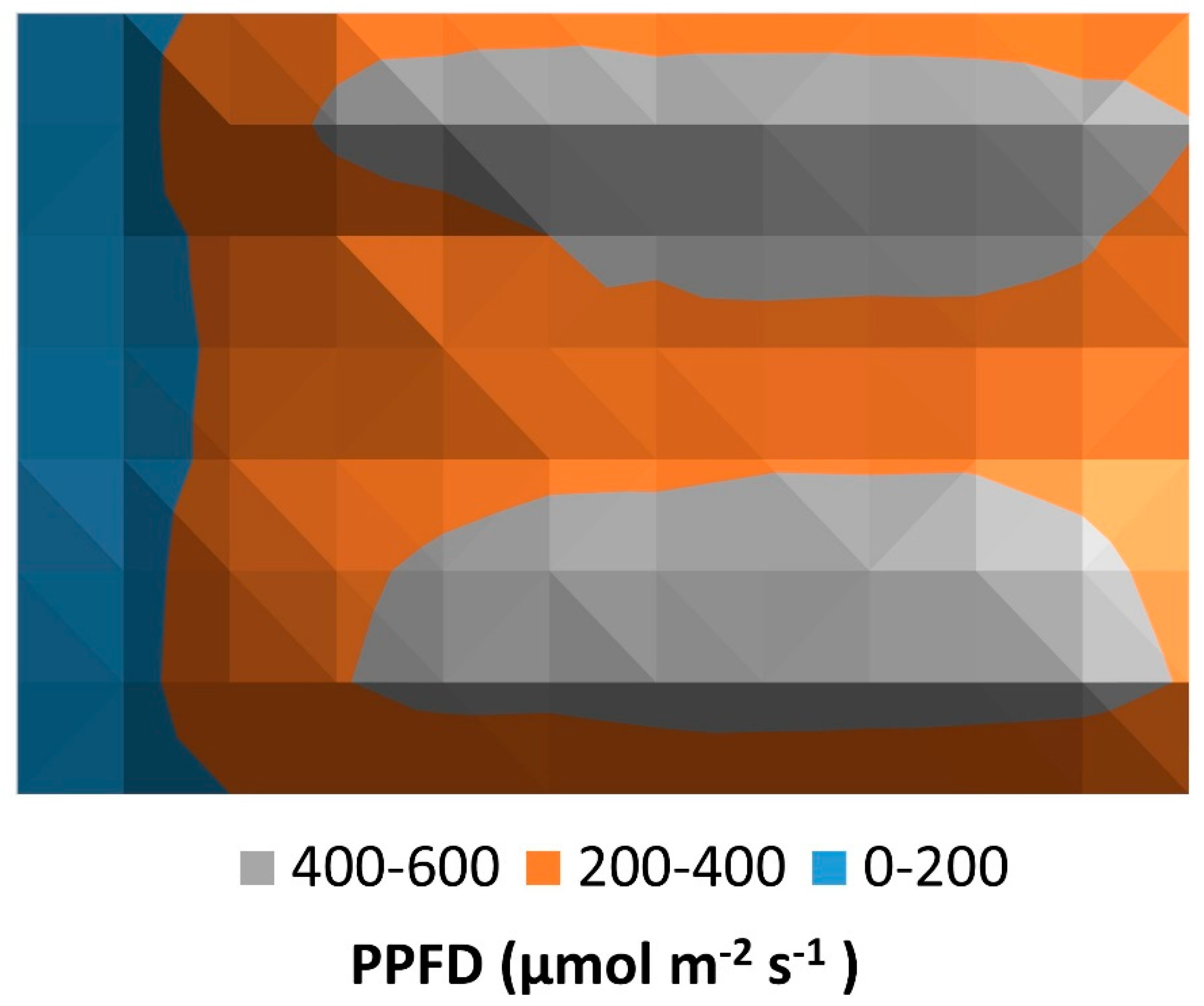
The experiment in this study was conducted based on a randomized block design of the four crops at three different photosynthetic photon flux density (PPFD{ XE “PPFD” \t “Photosynthetic photon flux density” }) (µmol m−2 s−1) levels. The artificial lighting of the SOF was analysed more closely, because energy is a major input and thus a main contributor to the operating expenses of indoor farming units [22]. The PPFD at crop surface level was determined in a preliminary experiment using a PPFD meter (Quantum meter MQ-200, Apogee). This measurement revealed considerable differences in PPFD level at plant level as shown in Figure 4.
Taking this into account, three blocks with three different PPFD levels (0–200/200–400/400–600 µmol m−2 s−1) were established to get a more adequate picture of light as a key factor for plant growth. Consequently, each of the four different crops was cultivated under each PPFD level in two repetitions. In order to maximize the light intensity for the crops, the dimmable LED units were set to 100% PPFD{ XE “PPFD” \t “Photosynthetic photon flux density” }.
The first block had a low PPFD with an average of 185.2 µmol m−2 s−1. The second had a medium PPFD with an average of 355.7 µmol m−2 s−1 and the third had a high PPFD with an average of 466.4 µmol m−2 s−1. The total average of PPFD was 335.8 µmol m−2 s−1 (Table 1).
For this experiment, all LED lights were switched on for 16 h per day, which resulted in an average daily light integral (DLI{ XE “DLI” \t “Daily light integral” }) of 19.3 mol m−2 d−1. The DLI is a useful unit when describing the light environment of plants, since it illustrates the rate of photosynthetic active radiation (PAR{ XE “PAR” \t “Photosynthetic active radiation” }) distributed to the plants over a 24 h period [23]. The first block had a DLI of 10.6 mol m−2 d−1. The second block had a DLI of 20.5 mol m−2 d−1 and the third block had a DLI of 26.6 mol m−2 d−1. All light conditions are summarized in Table 1.
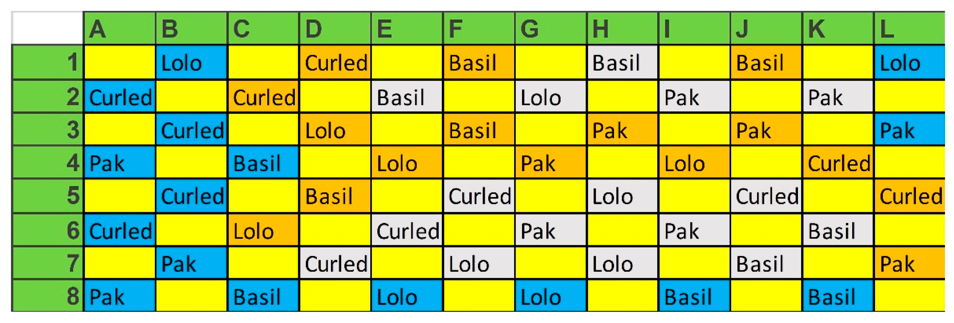
All planting spaces were sorted by PPFD and divided into three blocks with the same number of planting spaces. The final distribution of plants per PL after randomisation and block construction is shown in Figure 5.
Subsequently, four crops were cultivated on 36 mm Grodan rockwool blocks. For each PL, 48 substrate blocks were used, which resulted in a total usage of 144 planting spaces. The planting spaces marked in yellow in Figure 5 were not planted, in order to provide space for crop development.
Curled lettuce, lolo rosso and pak choi were cultivated as typical leafy greens and basil was the selected herb. Lettuce was chosen because of its fast growth and because it is cultivated worldwide, making it one of the most consumed leafy vegetables [24]. Basil was chosen because it can be found in most supermarkets and has been used as a spice and medicinal plant for ages [25]. A production cycle of five weeks was chosen from sowing till harvest, which is typical for lettuce and basil in indoor environments. In total, 12 plants of each crop were grown per production level at different PPFD levels. In order to minimize loses of productivity and because the germination rate in the faming unit was not known, 2–3 seeds of curled lettuce, lolo rosso and pak choi were sown per substrate block. For basil, 3–5 seeds per substrate block were sown. All seeds were sown by hand directly into wet rockwool plugs and subsequently transferred into the SOF according to the cultivation plan (Figure 5).
The crops were cultivated using municipal tap water. The pH and the electrical conductivity (EC) were adjusted at the beginning of the experiment and during the experiment about once a week. The pH was maintained between 5.5 and 6, because nutrients are optimally available [26,27]. During the experiment, however, the pH ranged between 4.8 and 6.8 due to manual adjustment using pH-up (nitric and phosphoric acid) and pH-down (potassium carbonate and silicate) (Terra Aquatica from General Hydroponics Europe). The EC value in the nutrient solution was steadily increased after the germination phase (about 5 days) to reach the crops’ demands, allowing for a fast production cycle and the intended consumption as babyleaf lettuce. A three-component fertilizer was used with the following N-P-K concentration: Remo Nutrients ‘Grow’ (2-3-5), ‘Magnifical’ (3-0-0) and ‘Micro’ (3-0-3) [28]. Initially an EC of 800 µS cm−1 was chosen for the principal growth stage 1, which was terminated after 6–9 leaves per plant were developed. After 21 days, the EC was raised to 1300 µS cm−1. It ranged from 1050–1300 µS cm−1 throughout the experiment. Regular measurements showed that the temperature always remained between 28–30 °C in PL two and 26–28 °C in PL one. Air humidity was 50–60% in PL two and 80–90% in PL one.
2.3. Techno-Economic Analysis
The techno-economic analysis performed here consists of: (i) a material flow analysis, following the approach of [29], and (ii) economic analysis following [30].
2.3.1. Material Flow Analysis
For the material flow analysis, all inputs that entered the SOF from planting stage to harvest of the crops were measured and recorded. These parameters included the amount of substrate, seeds, water, fertilizer, pH buffering solution and the energy for lights, pumps and monitoring devices. During the experiment, the water usage was measured by recoding the water level in the tank before and after filling. The energy consumption was measured with an electric meter (Energy Check 3000, Voltcraft, Hirschau, Germany). The weight and number of substrate blocks was measured with a scale (AMIR, DE-KA6). Fertilizer and pH buffer usage was documented over the whole period.
At harvest, the total fresh matter (FM{ XE “FM” \t “Fresh matter” }) yield of consumable biomass was considered as output. However, the FM{ XE “FM” \t “Fresh matter” } yield of all four crops produced in the two PLs with three PPFD levels was measured in order to analyze the yield per PL and PPFD level. This resulted in 24 different biomass samples at harvest. The biomass samples were dried in a drying oven (VTU 125/200, Weiss Technik GmbH, Reiskirchen, Germany) at 60 °C for 24 h to obtain the dry matter (DM) yield as well.
The productivity of PL 1 and PL 2 was analyzed and checked for significant differences due to different cultivation conditions with a paired t-test in Microsoft Office XP Excel.
Furthermore, the theoretical productivity of the farming unit was determined in four different scenarios assuming that one of the crops would have been cultivated in monoculture.
2.3.2. Economic Analysis
For the economic analysis, all prices for the input factors from the material flow analysis were determined and the total operating expenses (OPEX) of the SOF were calculated. This allowed for the determination of the production costs kg−1 consumable biomass.
In order to account for the possibility of operating an indoor farming unit on renewable energy two scenarios were made, distinguishing between conventional (EUR 0.2925 kWh−1) and renewable (EUR 0.2768 kWh−1) electricity prices. Subsequently, all cost factors were summarized and ranked based on their relative contribution to the total operating expenses.
3. Results
First, the results of the material flow assessment are presented and second the economical assessment.
3.1. Material Flow Assessment
First, the inputs of the SOF were determined in Section 3.1.1, followed by the outputs in Section 3.1.2 An overview of the results of techno-economic assessment of the SOF is provided in Figure 6.
3.1.1. Input
The inputs include seeds, substrate, fertilizer, pH-buffer, water and energy. The amounts used were documented along with the prices (Figure 6).
Seed Usage
Fertilizer Usage
Over a period of 5 weeks, 202.5 mL fertilizer was used. The total fertilizer costs account for EUR 2.39 in the experiment (Table 3).
The combined content of added nutrients is summarized in Table 4. The remaining nutrients after production were not assessed.
pH-Buffer Usage
Over the production cycle, 103.06 mL pH-down and 11.16 mL pH-up buffering solution were used. The costs of buffering solutions were EUR 2.25 for the whole production cycle (Table 5).
Water Usage
In total, 143.28 L of water were consumed (Table 6). The water usage over the production cycle is shown as weekly cumulated values in Figure 7. In the beginning, the water usage was low and increased substantially later on (Figure 7). The total average water consumption was 4.1 L d−1 at a temperature of 28–30 °C maintained in PL two and 26–28 °C in PL one and air humidity of 50–60% in PL two and 80–90% in PL one.
Energy Consumption
The total energy consumption of the SOF (extrapolated to all three PL) for one production cycle of five weeks was 270.5 kWh or 973.8 MJ. This results in an energy input per produced kilogram biomass of 496.4 MJ kg−1 FM or 2977 MJ kg−1 DM (considering electricity inputs only, while omitting energy required for material and fertilizer production).
3.1.2. Output
First, the total consumable biomass yield (fresh matter and dry matter) was analysed for the entire SOF surface and then calculated on a square meter basis. Second, the fresh matter and dry matter yields of the different crops were analysed and compared for the three PPFD levels. Third, the biomass yields of the two PL were statistically compared. Additionally, a scenario analysis was performed to calculate the potential yields for the four individual crops of this experiment in the SOF.
The total fresh matter yield of the four crops, extrapolated to the entire SOF, was 1961.8 g per 0.79 m2. This converts to 2473.9 g m−2. Pak choi had the highest potential yield with 676.8 g and basil had the lowest potential yield with 363.8 g, which is 53.8% less (Table 7).
The individual yields of the four crops under the three PPFD blocks are summarized in Table 8. The lowest yield was measured for basil (24.1 g) on PL 1 at low PPFD level. The highest yield was obtained from pak choi with 105.9 g at intermediate PPFD level on PL two. Looking at PL two, curled lettuce and lolo rosso grew better with increasing PPFD level. On PL one, lolo rosso yield increased slightly the higher the PPFD was, while the yield of curled lettuce decreased with stronger PPFD. Pak choi had a peak at the intermediate PPFD again and basil yield was increasing with higher PPFD.
Furthermore, dry matter (DM) yields have been analyzed (Figure 8). Pak choi produced the highest DM yield and lolo rosso the lowest. The total DM yield of the SOF was 172.3 g DM. All DM yields increased with higher PPFD, except pak choi, which had the highest DM at intermediate PPFD level.
Subsequently, the productivity of both production levels was compared in order to assess whether the growth conditions were similar on the different PL. The total yield for the two PL was 1307.9 g FM per 0.79 m2. However, PL one yielded 530.3 g FM, while PL two had a 46.6% higher yield with 777.5 g FM. The yield differences between the four crops on the two production levels at varying PPFD levels are displayed in Figure 9. It shows that PL 2 always produced higher yields at all PPFD levels.
A two-tailed paired t-test resulted in the rejection of the assumption that both production levels delivered the same output since P was higher than alpha (0.05). The results of the two-tailed paired t-test are shown in Table 9. The comparison revealed that the cultivation conditions varied significantly between the two layers.
In addition, the yield of the individual crops was extrapolated to the whole farm, assuming that only this crop would have been cultivated. This resulted in four scenarios revealing the crop with the highest potential biomass yield (Table 10). Scenario three (pak choi production only) would attain a FM yield of 2707 g, which is the highest potential yield. On the contrary, scenario four (basil production only) would result in 1455.2 g, the lowest yield of all crops.
For comparison of the biomass yield of the SOF with yield levels of other in- and outdoor biomass production systems, the productivity of the SOF was converted to Mg FM per hectare and year. The SOF has a total surface area of 0.79 m2 (1.38 m × 0.7 m). The production cycle of five weeks would potentially allow for up to 10 harvests.
The yield levels on hectare basis are shown in Table 11. A total FM yield of 257 Mg FM ha−1 year−1 is potentially achievable with the four crops used in this study. Considering the cultivation of pak choi (scenario 3) only 355 Mg FM ha−1 year−1 would potentially be possible. The production of only basil (scenario 4) would lead to the lowest potential yield of 191 Mg FM ha−1 year−1.
3.2. Economic Assessment
The total input costs of the SOF were summed up to determine the price per kg consumable biomass produced in the SOF (Figure 6). The operating expenses (OPEX) for all production factors (without labor) and inputs are summarized and ranked based on their relative contribution to the total OPEX (Table 12 and Table 13). Energy accounts for more than 70% of the OPEX. Considering this, the results are shown with the electricity price of electricity from renewable sources only (Table 12) and the conventional electricity mix of Germany (Table 13).
Fixed costs and labor costs were neglected because the latter can vary considerably and the intended users in offices would perform the maintenance as a hobby during their breaks. The fixed costs can hardly be estimated for an SOF at prototype stage.
When using renewable energy, total OPEX result in EUR 104.3 per five-week production cycle (Table 13). The main input was renewable energy (270.5 kWh) with EUR 74.9, representing 71.8% of the total costs. Rockwool as cultivation substrate accounts for EUR 15.5 and contributes the second highest share (14.8%) to the production costs, followed by seeds, fertilizer, and pH buffer. Water usage had the lowest impact on total costs, with EUR 0.3 and 0.6% of total costs.
With conventional energy, the total production costs were EUR 108.23 per five-week production cycle, with energy accounting for EUR 79.12 and 73.1% of the total production costs.
Overall, the cultivation of one kilogram of the four crops over five weeks results in total OPEX of EUR 53.14 when using renewable energy, while one kg of biomass grown with conventional energy costs EUR 55.17. In this case, the more sustainable renewable energy from the local power utility is also 3.7% cheaper than conventional electricity.
4. Discussion
The techno-economic assessment of the SOF is discussed with respect to (i) the technical setup and the design of the SOF (Section 4.1), (ii) the implications for cultivation management (Section 4.2) and (iii) the resource use and the productivity of the SOF compared to traditional field, greenhouse production and professional vertical farming units (Section 4.3).
4.1. Productivity
In the following section, the mixed scenario will be compared to the average lettuce production worldwide, to the average field and greenhouse lettuce production in Germany and the average field production in Baden Württemberg. Such a comparison with yields under field conditions is important to put the results of the indoor farming approach into perspective. A similar approach was also carried out by Wittmann et al. [31], who studied an indoor vertical farming method for marjoram production. Additionally, the lettuce yield will be compared with a greenhouse in Switzerland and a vertical farm feasibility study of the German Aerospace Centre (DLR). Finally, published yields of existing vertical farms such as Aerofarms, Plenty, Infarm and Skygreens were regarded.
The yield of the SOF in this study was 2473.9 g m−2 5 weeks−1. Since the SOF can produce all year long, 257 Mg FM ha−1 year−1 of mixed crops are potentially possible. In comparison, the mean yield for lettuce production worldwide in the year 2017 was 21.9 Mg FM ha−1 year−1 and the mean yield of lettuce produced in Germany in the year 2019, under field conditions, was 25.8 Mg ha−1 for lolo rosso, 25.5 Mg ha−1 for curled lettuce and 33.3 Mg ha−1 for cabbage lettuce [32]. The mean yield of romaine lettuce (Lactuca sativa var. longifolia) was 36.1 Mg ha−1, while cabbage lettuce (Lactuca sativa var. capitata L.) yield was 42.6 Mg ha−1 under field conditions in Baden Württemberg (Germany) in 2019 [33,34].
In a greenhouse in Switzerland, Marton [35] found that cabbage lettuce yield was 48.1 Mg ha−1. Zeidler et al. [36] calculated potential lettuce yields in a feasibility study of the vertical farm “EDEN”. They found that a yield of 6436.2 g m−2 5 weeks−1 is possible, which results in 669.4 Mg FM ha−1 year−1 with a minimum price of EUR 12.5 kg−1 of biomass.
Aerofarms in the US, one of the leading vertical farming companies, for example, says that they can produce 390-times more than conventional agriculture [37] and Skygreens in Singapore claim a 10-times higher yield in comparison to conventional agriculture [38]. Infarm, a Berlin based vertical farming company, mentioned that 400 times higher yields are possible [39] and Plenty, a San Francisco based vertical farming company, claims that 350 times higher yields are possible [34]. The mean world production of lettuce was used as a core value and multiplied with the claims of the vertical farming companies to give an overview. Toledano et al. [40] estimates that current market prices for one kg of leafy greens are around USD 33 for vertically-grown produce. When comparing the productivity, it is shown that the mean lettuce production has the lowest productivity and that Infarm has the highest claimed productivity with 8760 Mg FM ha−1 year−1 (Figure 10). Thus, field conditions are less productive than greenhouse conditions and vertical farming conditions are even more productive.
The SOF has a smaller productivity than bigger farms since effects of scale are small, management is less efficient and resource use is high, making the production not economical viable at the moment. However, on the other hand, this trial implied only one production cycle and the cultivation measures and technical aspects of the farming unit can be improved with increasing experience with the SOF.
The agricultural sector could become more decentralized if similar farming units would be installed in many places. However, for the efficient use of such indoor farming units, they might need more plant production knowledge and the distribution of produced crops would need to be managed efficiently. This is a call for some kind of digital platform, which manages data, processes and resource flows and professionals, which can support and educate producers to make production economically viable.
From an economic point of view, one kg of biomass produced in the SOF costs EUR 53.1 and thus was more expensive than reported by Zeidler et al. [36] (EUR 12.5) and Toledano et al. [40] (USD 33). This is due to the rather low productivity compared to commercial indoor cultivation units (e.g., Infarm) and large-scale vertical farms (e.g., Plenty, Aerofarms). A closer look at the technical setup of the SOF and the cultivation conditions of this study can provide explanations for these yield differences and strategies for optimization of the SOF.
4.2. Technical Aspects
The technical design of the SOF revealed significant differences in growth conditions between the two production levels with respect to irrigation and fertilization as well as temperature and relative humidity. Based on this, future improvements of the SOF have been elaborated with respect to irrigation and fertilization (Section 4.2.1) as well as climate control (Section 4.2.2) in order to optimize SOF productivity.
4.2.1. Irrigation
The irrigation and fertilization of crops in soilless cultivation systems determine crop productivity to a large extent. The irrigation setup determines the supply of the plants with water and nutrients [41,42]. Keeping the EC and pH levels at crop specific optima is highly important for achieving high productivity in hydroponics and even small misconfigurations in irrigation, fertilization and pH level can lead to the total failure of the crops [16]). Automated monitoring and control of these cultivation factors are thus highly important, especially when untrained people, such as, e.g., in offices, operate the cultivation system.
The significant productivity differences between the two production levels can be attributed to differences in the irrigation regime. One reason might be the too small volume of the water tank in relation to the planting space, which does not allow for continuous irrigation of both production levels.
A larger water tank volume would additionally increase the pH buffering capacity, as small pH changes have direct impacts on nutrient availability [42]. With every irrigation cycle, the quantity of water, the nutrient composition and the pH change because plants take up water and nutrients and return metabolic products. The larger the volume of the tank, the smaller the impact of changes on EC, pH and water. Sufficiently large water reservoirs are important in hydroponic crop cultivation, reducing the dependency on the exact dosage of pH-buffering solution and fertilizer, making the amplitude of changes of EC, pH and water amount smaller and improving crop cultivation conditions [43]. This could improve plant health and increase biomass yields and decrease the maintenance requirements of indoor farming units [44].
Furthermore, it was observed that PL one received less water that PL two, which is located above PL one. The resulting differences in pump resistance due to different heights had to be carefully managed through manual valves in this study. A second improvement possibility would thus be a different configuration of water inflow and outflow. A solution would be a more precise dosage of water and nutrients to each PL, which can be conducted through modification of the valves for in and outflow. A larger water reservoir paired with flow sensor-based magnetic valves would allow for an automated control of the irrigation and fertilization regime of both production levels and can thus improve overall productivity of the SOF.
A third option would be a change in irrigation style, once a larger water reservoir would be installed. The current setup does only allow for very short ebb and flow cycles with pumping times of a maximum of two minutes. Maybe longer flow cycles or the shift towards nutrient film technique (NFT) would result in a higher and more even productivity of the two layers.
4.2.2. Climate Control
The differences in temperature and relative humidity may explain the varying productivity between the two production layers [45]. Plants are an integral part of the soil–plant–atmosphere continuum (SPAC{ XE “SPAC” \t “soil-plant-atmosphere continuum” }). The water gradient between the atmosphere of the office and the nutrient solution of the SOF is a main driver for plant transpiration and nutrient absorption [46]. Additionally, temperature in the office and thus inside the SOF (without climate control) plays a vital role in plant physiology [16]. Hence, the relative humidity of the SOF determines plant growth and may even cause phytopathogenic problems (see Section 4.3). For optimizing relative humidity and the microclimate at each production level of the SOF, a controlled airflow would be a solution. The additional installation of a sensor-based temperature and relative humidity control system with fans and defined temperature and humidity benchmarks adapted to crop requirements can improve productivity and resource-use efficiency.
Following the assumption that the use case for the SOF is an office with relatively low air humidity, an adjustable airflow from the inside of the farm to the outside of the building might decrease relative humidity inside the SOF (and the office room) and thus increase plant transpiration and nutrient uptake for faster growth. If this is not possible, e.g., due to high installation costs, sensor-controlled air circulation at each production level should be installed.
In addition, evaporation should be minimized to reduce water losses. Therefore, the planting trays should cover the production levels completely for as little direct contact with the air as possible.
The role of the CO2 concentration has not been considered in this study, but should be investigated further, because beneficial outcomes for humans and plants are possible when CO2 from the office (as a product of human transpiration) is provided as a resource to the crops [47].
Consequently, the productivity and resource-use efficiency of the SOF can be optimised by a larger water reservoir, enabling NFT cultivation, an improved water and nutrient distribution to the production levels and controlled temperature and relative humidity. The technical adaptations additionally facilitate crop production by untrained users, rendering the SOF a viable option for the automatized crop cultivation in offices.
4.3. Cultivation Measures
The applied cultivation measures in this experiment were determined by the technical setup of the SOF. Here, the implications of temperature and relative air humidity, pH and EC and the chosen production cycle are discussed in detail. Furthermore, adjustments in these parameters are discussed in order to optimize productivity.
4.3.1. Temperature and Relative Air Humidity
Following the discussion about the technical setup for climate control in Section 4.2.2, here, the actual values of the temperature and relative humidity of this study are examined and discussed in detail. Regular measurements of the installed sensors showed that the temperature inside the SOF was always between 28–30 °C in PL two and 26–28 °C in PL one. Relative air humidity was 50–60% in PL two and 80–90% in PL one.
Ahmed et al. [48] suggest a temperature of 22–25 °C during the light period and 70–80% relative air humidity to be optimal for lettuce cultivation. The differences in temperature and relative air humidity can partly explain the yield different between the two PLs [45], in addition to the difference in received water and nutrients, discussed in 4.2.1.
The suboptimal relative air humidity also led to symptoms of calcium deficiency, which were detected in young basil leaves of this study. Palzkill et al. [49] showed many years ago that high relative air humidity can cause calcium deficiency.
Overall, the suboptimal temperature and air humidity, which cannot be controlled so far, are subject of improvement through the installation of a sensor-controlled forced airflow technology. This measure can optimize productivity and thus decrease production costs of the SOF.
4.3.2. EC and pH
EC and pH of the nutrient solution are another two important factors for crop production. Essentially, the EC is a measure for concentration of plant nutrients (not about the composition), while the pH largely determines their plant availability.
Ding et al. [50] showed that the fresh and dry weight, and the leaf size of pak choi plants increased with higher EC values. Highest pak choi yields were achieved at an EC of 4800 µS cm−1 [50]. This reveals that the EC of this study (max. 1300 µS cm−1) was too low for pak choi. This further indicates that pak choi is not suitable for polyculture with low-demanding lettuce and basil.
Walters and Currey [51] showed that for basil EC levels from 500 to 4000 µS cm−1 did not affect plant growth, but it was affected by increasing DLI from about 7 mol·m−2·d−1 to about 15 mol·m−2·d−1. In this study, the DLI was even higher with 19.3 mol·m−2·d−1. Basil plants with low EC and high DLI showed no significant difference to plants with high EC and high DLI in terms of fresh matter [51]. Consequently, the EC and DLI set in the SOF were in the optimal range for basil cultivation.
The optimal pH range is generally assumed to be between 5.5 and 6 because nutrients are optimally available [26]. However, Gillespie et al. [27] showed that a pH of 4 in the nutrient solution can contribute to better plant health by reducing root rot severity in basil plants [27]. In the SOF, automated fertilizer and pH buffer dosing can keep pH and EC levels more stable and within the optimal ranges for particular crops. Despite the additional costs for this technical adaptation, a higher productivity of the SOF can be expected [30,52].
4.3.3. Production Cycle
A ‘production cycle’ refers to the time the crops are cultivated from seed or seedling to harvest and is determined by the producer and the desired product. It can range from a couple of days (e.g., for microgreens) to several months (e.g., herbs). The length of production cycle influences yield, morphology, content of nutrients, vitamins and other secondary metabolites of the crop parts and whether the plant is in its vegetative or generative phase. A multitude of social, ecological and economic factors determine the production cycle chosen by a producer.
For this experiment, it was assumed that a group of office workers has different food preferences, which can be met best with a polyculture and a rather short production cycle of five weeks till harvest. Thus, the harvest time of basil, curled lettuce, lolo rosso and pak choi were combined.
As a consequence, basil grew too tall, and some plants touched the LED unit resulting in burned tips of the uppermost leaves. In the trial, three to five basil seeds were sown per rockwool plug. Basil varieties with a more compact morphology can be used in the future if a polyculture will be cultivation in the SOF. Furthermore, a higher sowing density can probably reduce the size of the basil plants per substrate block. Lettuce plants were small in comparison to commercially grown lettuce. The average fresh matter of lolo rosso and curled lettuce was 71.5 g in the SOF, which is much less than the average selling weight of about 170 g in Germany [53]. For lettuce, a longer production cycle of about 10–14 days would have resulted in much higher yields, since lettuce plants were just at the beginning of their major growth phase at harvest time [54].
Consequently, the production cycle largely determines the productivity of indoor farming units, while the intended use of a crop (or certain parts or ingredients) in turn determines the production cycle and economic viability.
4.4. Resource Use
Urban areas have great potential for the increase in resource-use efficiency in terms of energy, materials (e.g., nutrients, water) and information and can at the same time contribute largely to a reduction in the impacts on environment and climate [55]. Decentralized food production through urban farming can increase the reuse and circulation of resources through the production of food, while providing improved access and availability to fresh and healthy food at low food miles [5,16,18]. High quality and nutritious food can be cultivated, e.g., in urban offices. Thereby, the consumer of food becomes the producer and values his own products potentially more than purchased food. This might also decrease the high share of food waste caused by consumers of up to 25% of the total food produced [56]. To turn cities sustainable through urban farming, resource flows need to circulate in the city [5]. In future, crop nutrients need to be derived from urban organic wastes. For example, Stoknes et al. [57] demonstrated that the vegetable and mushroom production from organic waste nutrient recovery is possible with the same or even higher yields. A shift from mineral-fertilizer-based hydroponics towards organic cultivation requires new approaches such as the terrabioponic cultivation currently used for outdoor urban gardening [58]. However, large scale food production based on nutrient and water recovery from urban organic wastes requires more research and development efforts in order to close the loops in resource flows [4].
4.4.1. Energy Consumption
Energy consumption determines the food production costs to the largest extent, with 73.1% of the total costs when conventional energy is used and 71.8% of the total costs when renewable energy is used. Therefore, energy can be seen as the main production factor in this experiment and in indoor urban farming generally [5,16]. The comparison of the renewable and conventional energy scenarios showed a small difference of 3.7% in this study. For improving the sustainability of urban indoor farming, the decrease in the energy consumption is of the highest importance. In this case, there is monetary incentive to utilize renewable instead of conventional energy. Energy self-production, e.g., on the roofs and facades of the building wherein the indoor farming unit is located, could improve the energy situation and render indoor food production more sustainable [59].
When considering the energy input (referring to electricity only), it becomes evident that 496.4 MJ kg−1 FM or 2977 MJ kg−1 DM are enormously high. Grain production through conventional agriculture shows energy inputs several orders of magnitude lower, with 5.3 MJ kg−1 grain for soybean, 3.3 MJ kg−1 grain for wheat and 2.6 MJ kg−1 grain for maize [60]. Modern greenhouse production cycles, comprising tomato, pepper and cucumber production in sequence (including tomato nursery), show average energy inputs for crop production (including all byproducts) ranging from 1.9 to 2.7 MJ kg−1 FM (total above ground biomass yield) [61]. These figures reveal the tremendous energy inefficiency of indoor crop production in small units such as the SOF.
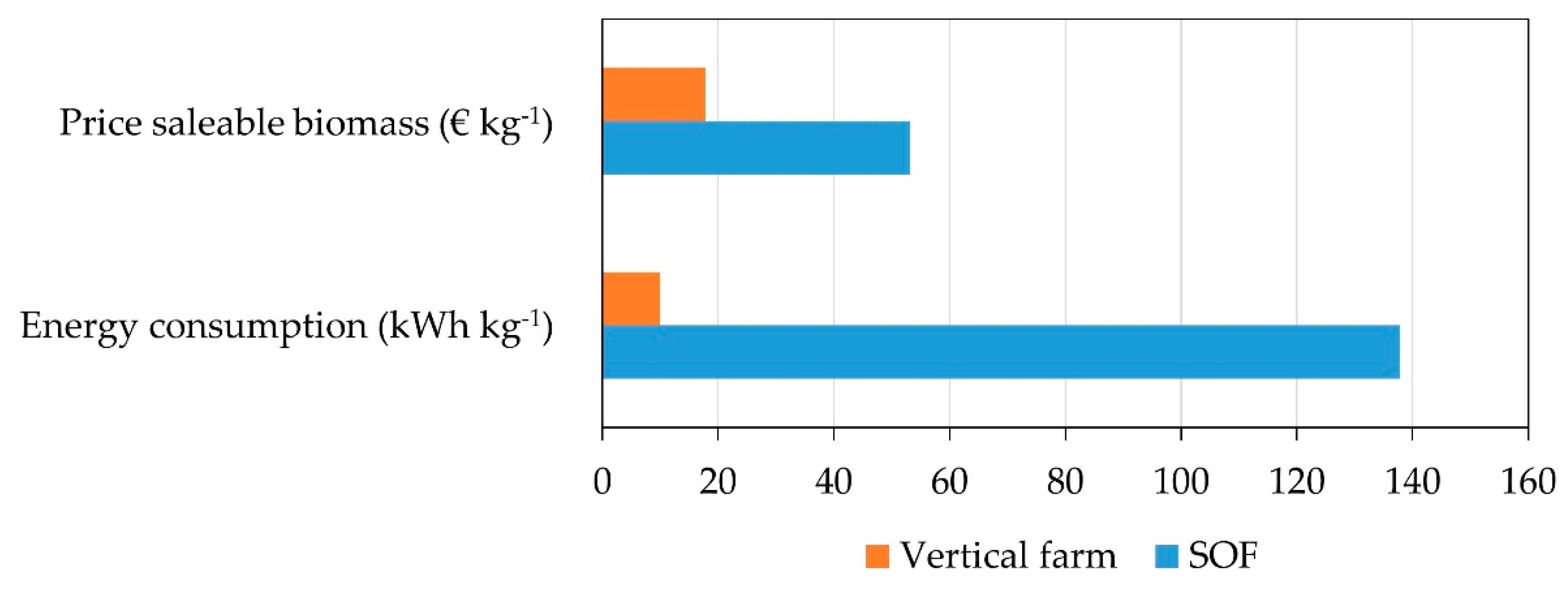
At present, lettuce production in large-sale modern vertical farming requires about 10 kWh (36 MJ) kg−1 harvested fresh biomass on average [16]. The SOF, however, consumed 137.9 kWh kg−1 edible fresh biomass (Figure 11). Consequently, the SOF requires 13.8 times more electricity. If the energy usage of the SOF could be reduced by 13.8 times through technical optimizations and improved cultivation management, this would decrease total production costs and make the relative impact of energy on the costs substantially smaller. In the scenario where renewable energy was used, total energy costs were EUR 74.9 and accounted for 71.8% of costs. When decreased by 13.8 times, energy costs would be EUR 34.8 and account for only 15.6% of costs. Looking at the price per kg of biomass, it would decrease from EUR 53.1 kg−1 to EUR 17.7 kg−1, thus cutting costs by 66.6%.
In particular, artificial lighting, which is not used in open-field agriculture and greenhouse production, is responsible for the high energy inputs in indoor farming units [5,16]. The use of or the self-production of renewable energy currently provides the most promising way to increase energy efficiency and render indoor farming a more viable and sustainable option for food production.
In addition, efficient usage of light through optimal PPFD values is of high importance for increasing the energy use efficiency and economic viability of indoor crop production. For the plants cultivated in this study, the optimum in PPFD is considered 200–250 µmol m−2 s−1 with a photoperiod of 16–18 h [22,48]. The arrangement of the LEDs should be adjusted to achieve an adequate and more equal PPFD distribution over the whole production area for optimizing crop productivity. In case of the SOF, the LED units should be longer to span over the whole production surface, while the PPFD output should be adjusted to the crop cultivated (which is already possible through dimming). PPFD levels above crop requirements, as was the case for pak choi in this study, increase production costs unnecessarily and reduce economic viability. Furthermore, crop arrangement in polyculture should be conducted according to the light demand of the crop. Crops with high light demand (e.g., lettuce in this study) should be placed directly under the light source, while crops with lower light demand can be placed in between the light sources (such as, e.g., pak choi in this study). Basil growth depends strongly on PPFD level and DLI [51], but grew too large in shoot length in this study resulting in tip burning, and, as such, should be placed between the LED stripes and the shoot may be cut at an early stage to trigger branching of the plant. The latter increases the cultivation cycle, but results in more shoots and harvestable leaves to be picked over a longer period of time. When basil is grown in polyculture, this could further help to adapt the harvest time to other crops with a longer production time.
The importance of LEDs, to decrease energy consumption and make production economically viable, increased since LEDs have a variety of advantages over traditional forms of horticultural lighting and a more efficient performance and longevity compared to any traditional lighting system [62]. Their small size, durability, long lifetime, cool emitting temperature and the option to select specific wavelengths for a targeted plant response make LEDs more suitable for plant-based uses than many other light sources. Furthermore spectral quality of LEDs can have dramatic effects on crop anatomy and morphology as well as nutrient uptake and pathogen development [63]. Global LED use has increased in recent years, since a market share of 5% in 2013 grew to nearly 50% of lighting sales in 2019 [64].
Whether the wavelengths of the LED units are optimal for this use has not been analyzed, but represents another promising option for optimizing resource use efficiency of indoor farming units such as the SOF.
Fixed costs have been neglected in this assessment because it is the prototype stage. However, it has to be noted that LED units are the part of the SOF with the highest individual costs [14].
Artificial lighting represents the driver for optimizing productivity in indoor farming units and reducing the production costs. Both energy inputs and production costs of small production units, such as the SOF, were found to be very high compared to large-scale modern vertical farming. From this assessment, it remains questionable whether office-based farming is a viable and sustainable option for urban production and more research and development efforts are necessary to substantially improve resource use efficiency.
4.4.2. Substrate
The cultivation substrate (rockwool) had a share of 14.3% (conventional energy) and 14.8% (renewable energy) of the total production costs of the SOF. When it comes to the choice of substrate, there are several options. Substrate fulfills three main functions in hydroponic cultivation systems, typically applied in modern indoor farming: (1) provide oxygen, nutrients and water to the roots, (2) allow for root growth and (3) support the stability of the crop [65]. Essentially, an optimal cultivation substrate must have a structure capable of providing a balance of oxygen and nutrient solution both during and between irrigation events to the roots [66,67].
Cultivation substrates can be categorized as organic, for example, peat and coconut coir, and inorganic components, for example, rockwool. Since peat and rockwool have large negative impacts on the environment, peat mining destroys wetlands, while rockwool can hardly be reused and recycled but production is very energy-intensive, current research and development focuses on organic residues from agriculture and organic waste products from biobased industries [68,69]. This can reduce environmental impacts and increase sustainability of indoor farming. In addition, organic substrates can be integrated into local material flows.
4.4.3. Seed Usage
The third biggest factor contributing to costs were the seeds, with shares of 5.9–6.1% on the total costs.
In this experiment, two to three seeds of curled lettuce, lolo rosso and pak choi were sown per substrate block. Whereas three to five seeds per substrate block were sown for basil. All seeds were sown directly into the wet rockwool plugs and then subsequently transferred into the SOF. Direct sowing into rockwool plugs showed fast and homogenous germination with minimum productivity losses and can thus be recommended for the operation of the SOF.
Additionally, a good choice of varieties is crucial in order to optimize yields. For example, basil had 53.8% less consumable biomass yield than pak choi, which is important to consider if maximal biomass yield is the objective. However, the aim of the SOF is to allow the consumer to cultivate according to her/his preference. Hence, direct sowing of crop combinations with similar growth requirements and automated cultivation in polyculture could be one of the use-cases of the SOF.
Since soil is not used in hydroponic production units, theoretically, diseases caused by soil-borne pathogens should not pose a problem [70]. Furthermore, under optimal indoor conditions, the whole environment can be controlled, and the production system can be closed. Hence, no pesticides are required under such conditions [16]. Pest management was not necessary in this study and was therefore not considered. Pesticide free production is a major asset of this type of cultivation system in terms of both consumer health and the environment.
4.4.4. Water Consumption
Vertical farming can be very water-efficient, with savings of up to 95% compared to open-field agriculture [71].
In this study, water had the lowest share on the total costs. One reason is the low water price in Stuttgart, Germany, another is the size of the unit and the recirculating ebb and flow cultivation system requiring only a small quantity of water.
In the future, efficient water usage will become more important since more than a quarter of the world’s population lives in regions which will have to cope with water scarcity [72], while Europe experienced one of the most severe droughts ever recorded in 2018 [73].
Therefore, it can be expected that the importance and the competitiveness of water-efficient production will increase and support the implementation of water efficient food production systems in urban areas.
5. Conclusions
Urban farming is part of the solutions for the intensification of food production with the aim of meeting the growing demand of the urban population. The cultivation experiment shows and confirms the high yield potential of smart indoor cultivation systems, while the techno-economic analysis of the SOF revealed very high production costs, mainly caused by very low energy-use efficiency compared to large-scale vertical farming (10 MJ kg−1 FM), modern greenhouse production (1.9 to 2.7 MJ kg−1 FM) and conventional open-field wheat production (3.3 MJ kg−1 grain).
The polyculture in the SOF yielded 1961.8 g on 0.79 m2 ground area, indicating a theoretical yield potential of 257 Mg FM ha−1 year−1 of edible and fresh biomass. However, as the economic assessment revealed, at production costs of EUR 53.10 kg−1 edible biomass in the renewable energy scenario (conventional energy EUR 55.17 kg−1). The most costly production factor is electricity (73%) for operating the SOF, followed by substrate (14%) and seeds (6%). Since energy is the main cost driver, urban indoor production should use renewable energy and requires further research and development to reduce its high energy demand.
Light is a crucial factor for (indoor) crop production. The yields of curled lettuce, lolo rosso and basil increased proportionally with increasing PPFD, except pak choi with a peak yield at the intermediate PPFD level (355.7 µmol m−2 s−1). Light distribution was very heterogeneous on plant level inside the SOF, revealing the need for optimizing PPFD at plant level to save energy and reduce production costs.
Small-scale cultivation systems, such as the SOF, for indoor food production are less productive and have lower energy-use efficiency than vertical farms. For the SOF, the effects of scale are small (e.g., smart, sensor-based control and operation unit for less than 2 m² productive area), the management is less efficient, and the resource-use is high, making food production not economically viable today.
However, this trial assessed a prototype SOF. The yield of this trial was low compared to vertical farming and modern greenhouse production and production conditions analyzed in the techno-economical assessment were found to be not optimal. Further trials are needed to optimize the SOF, focusing on technical improvement of the SOF and subsequently on developing optimal cultivation conditions and management with this particular indoor farm.
With improved resource-use efficiency and advanced cultivation management, the productivity of the SOF can be increased, rendering smart indoor cultivation systems such as the SOF a viable option to produce fresh and healthy food right at the place of consumption.
Author Contributions
Conceptualization, J.C., B.W. and M.v.C.; methodology, J.C. and B.W.; investigation, J.C. and B.W.; resources, J.C.; data curation, J.C. and B.W.; writing—original draft preparation, J.C., B.W. and M.v.C.; writing—review and editing, J.C., B.W. and M.v.C.; visualization, J.C. and B.W.; supervision, B.W.; project administration, J.C. and B.W.; funding acquisition, B.W. All authors have read and agreed to the published version of the manuscript.
Funding
This research received funding from the Ministry of Rural Affairs and Consumer Protection Baden Württemberg (14-(27)-8402.43/0405 E).
Institutional Review Board Statement
Not applicable.
Informed Consent Statement
Not applicable.
Data Availability Statement
Data sets of this research can be shared upon request.
Acknowledgments
The authors are very grateful to the Ministry of Rural Affairs and Consumer Protection Baden Württemberg, Jens, Florian and Steffen from farmee GmbH as well as Iris Lewandowski for making the SOF research work possible.
Conflicts of Interest
The authors declare no conflict of interest.
References
- Christensen, P.; Gillingham, K.; Nordhaus, W. Uncertainty in Forecasts of Long-Run Economic Growth. Proc. Natl. Acad. Sci. USA 2018, 115, 5409–5414. [Google Scholar] [CrossRef] [PubMed] [Green Version]
- Alexandratos, N.; Bruinsma, J. World Agriculture towards 2030/2050: The 2012 Revision. Available online: http://ageconsearch.umn.edu/record/288998 (accessed on 28 January 2021).
- United Nations; Department of Economic and Social Affairs; Population Division. World Urbanization Prospects: The 2018 Revision; 2019; Available online: https://population.un.org/wup/publications/Files/WUP2018-Report.pdf (accessed on 10 December 2022).
- Smit, J.; Nasr, J. Urban Agriculture for Sustainable Cities: Using Wastes and Idle Land and Water Bodies as Resources. Environ. Urban. 1992, 4, 141–152. [Google Scholar] [CrossRef] [Green Version]
- Al-Kodmany, K. The Vertical Farm: A Review of Developments and Implications for the Vertical City. Buildings 2018, 8, 24. [Google Scholar] [CrossRef] [Green Version]
- Clinton, N.; Stuhlmacher, M.; Miles, A.; Aragon, N.U.; Wagner, M.; Georgescu, M.; Herwig, C.; Gong, P. A Global Geospatial Ecosystem Services Estimate of Urban Agriculture. Earths Future 2018, 6, 40–60. [Google Scholar] [CrossRef]
- Specht, K.; Zoll, F.; Schümann, H.; Bela, J.; Kachel, J.; Robischon, M. How Will We Eat and Produce in the Cities of the Future? From Edible Insects to Vertical Farming—A Study on the Perception and Acceptability of New Approaches. Sustainability 2019, 11, 4315. [Google Scholar] [CrossRef] [Green Version]
- Goldstein, M.; Bellis, J.; Morse, S.; Myers, A.; Ura, E. Urban Agriculture: A Sixteen City Survey of Urban Agriculture Practices across the Country; Turner Environmental Law Clinic: Atlanta, GA, USA, 2011; pp. 1–94. [Google Scholar]
- Bio-Balkon.de Dein Balkon Als Essbare Wohlfühloase Für Mensch Und Tier! (Transl.: Your Balcony as an Edible Oasis of Well-Being for Humans and Animals!). Available online: https://bio-balkon.de/ (accessed on 10 December 2022).
- Geco-Gardens.de Ökologisch Gärtnern. Einfach & Überall. (Transl.: Garden ECOlogically Everywhere). Available online: https://geco-gardens.de/ (accessed on 10 December 2022).
- AeroFarms—An Environmental Champion, AeroFarms Is Leading the Way to Address Our Global Food Crisis by Growing Flavorful, Healthy Leafy Greens in a Sustainable and Socially Responsible Way. Available online: https://aerofarms.com/ (accessed on 10 December 2022).
- Zezza, A.; Tasciotti, L. Urban Agriculture, Poverty, and Food Security: Empirical Evidence from a Sample of Developing Countries. Food Policy 2010, 35, 265–273. [Google Scholar] [CrossRef]
- Artmann, M.; Sartison, K. The Role of Urban Agriculture as a Nature-Based Solution: A Review for Developing a Systemic Assessment Framework. Sustainability 2018, 10, 1937. [Google Scholar] [CrossRef] [Green Version]
- Ackerman, K.; Conard, M.; Culligan, P.; Plunz, R.; Sutto, M.-P.; Whittinghill, L. Sustainable Food Systems for Future Cities: The Potential of Urban Agriculture. Econ. Soc. Rev. 2014, 45, 189–206. [Google Scholar]
- McKenzie, F.C.; Williams, J. Sustainable Food Production: Constraints, Challenges and Choices by 2050. Food Secur. 2015, 7, 221–233. [Google Scholar] [CrossRef]
- Kozai, T.; Niu, G.; Takagaki, M. Plant Factory: An Indoor Vertical Farming System for Efficient Quality Food Production, 2nd ed.; Elsevier Inc.: Amsterdam, The Netherlands, 2020; ISBN 978-0-12-816691-8. [Google Scholar]
- McCormack, L.A.; Laska, M.N.; Larson, N.I.; Story, M. Review of the Nutritional Implications of Farmers’ Markets and Community Gardens: A Call for Evaluation and Research Efforts. J. Am. Diet. Assoc. 2010, 110, 399–408. [Google Scholar] [CrossRef]
- Pirog, R.; Benjamin, A. Checking the Food Odometer: Comparing Food Miles for Local versus Conventional Produce Sales to Iowa Institutions; Leopold Center Pubs and Papers: Ames, IA, USA, 2003. [Google Scholar]
- Hönle, S.E.; Meier, T.; Christen, O. Land Use and Regional Supply Capacities of Urban Food Patterns: Berlin as an Example. Ernahr-Umsch 2017, 64, 11–19. [Google Scholar] [CrossRef]
- Ohyama, K.; Takagaki, M.; Kurasaka, H. Urban Horticulture: Its Significance to Environmental Conservation. Sustain. Sci. 2008, 3, 241–247. [Google Scholar] [CrossRef]
- Lewandowski, I. Bioeconomy: Shaping the Transition to a Sustainable, Biobased Economy. p. 14. Available online: https://library.oapen.org/viewer/web/viewer.html?file=/bitstream/handle/20.500.12657/42905/2018_Book_Bioeconomy.pdf?sequence=1&isAllowed=y (accessed on 31 January 2021).
- Pennisi, G.; Blasioli, S.; Cellini, A.; Maia, L.; Crepaldi, A.; Braschi, I.; Spinelli, F.; Nicola, S.; Fernandez, J.A.; Stanghellini, C.; et al. Unraveling the Role of Red:Blue LED Lights on Resource Use Efficiency and Nutritional Properties of Indoor Grown Sweet Basil. Front. Plant Sci. 2019, 10, 305. [Google Scholar] [CrossRef] [PubMed] [Green Version]
- Faust, J.E.; Holcombe, V.; Rajapakse, N.C.; Layne, D.R. The Effect of Daily Light Integral on Bedding Plant Growth and Flowering. HortScience 2005, 40, 645–649. [Google Scholar] [CrossRef] [Green Version]
- Wiggins, Z.; Akaeze, O.; Nandwani, D.; Witcher, A. Substrate Properties and Fertilizer Rates on Yield Responses of Lettuce in a Vertical Growth System. Sustainability 2020, 12, 6465. [Google Scholar] [CrossRef]
- Dachler, M.; Pelzmann, H. Arznei-Und Gewürzpflazen; Agrarverlag Wien: Vienna, Austria, 1999. [Google Scholar]
- Alam, S.M. Effects of Solution PH on the Growth and Chemical Composition of Rice Plants. J. Plant Nutr. 1981, 4, 247–260. [Google Scholar] [CrossRef]
- Gillespie, D.P.; Kubota, C.; Miller, S.A. Effects of Low PH of Hydroponic Nutrient Solution on Plant Growth, Nutrient Uptake, and Root Rot Disease Incidence of Basil (Ocimum basilicum L.). HortScience 2020, 55, 1251–1258. [Google Scholar] [CrossRef]
- Remonutrients Base Nutrient Formulas. Available online: https://www.remonutrients.com/product/remos-micro-grow-bloom/ (accessed on 10 December 2022).
- Heck, P.; Bemmann, U. Praxishandbuch Handbuch Stoffstrommanagement 2002/2003; Deutscher Wirtschaftsdienst Köln: Koln, Germany, 2002. [Google Scholar]
- Lauer, M. Methodology Guideline on Techno Economic Assessment (TEA). In Workshop WP3B Economics, Methodology Guideline; 2008; Available online: https://www.scribd.com/document/333629930/Thermalnet-Methodology-Guideline-on-Techno-Economic-Assessment (accessed on 10 December 2022).
- Wittmann, S.; Jüttner, I.; Mempel, H. Indoor Farming Marjoram Production—Quality, Resource Efficiency, and Potential of Application. Agronomy 2020, 10, 1769. [Google Scholar] [CrossRef]
- Ertragsmenge von Salatsorten in Deutschland 2019. Available online: https://de.statista.com/statistik/daten/studie/639108/umfrage/ertragsmenge-von-salatsorten-in-deutschland/ (accessed on 22 March 2021).
- Zufriedenstellende Gemüseernte 2019—Statistisches Landesamt Baden-Württemberg. Available online: https://www.statistik-bw.de/Presse/Pressemitteilungen/2020033 (accessed on 18 February 2021).
- Plenty, 2021 About Us. Available online: https://www.plenty.ag/about-us/ (accessed on 22 March 2021).
- Marton, S. Ökobilanz von Gewächshausgurken Und Salaten. Stiftung myclimate—The Climate Protection Partnership, Zürich, Switzerland, 2010. Available online: https://www.researchgate.net/publication/228380499_Okobilanz_von_Gewachshausgurken_und_Salaten (accessed on 10 December 2022).
- Zeidler, C.; Schubert, D.; Vrakking, V. Feasibility Study: Vertical Farm EDEN. Available online: https://elib.dlr.de/87264/ (accessed on 18 February 2021).
- AeroFarms. 2021. Available online: https://aerofarms.com/ (accessed on 28 March 2021).
- Sky Greens. Available online: https://www.skygreens.com/ (accessed on 28 March 2021).
- Upshall, E. Infarm Unveils New Automated Growing Centre with Higher-Yield Capabilities. FoodBev Media 2021. Available online: https://www.foodbev.com/news/infarm-unveils-new-automated-growing-centre-with-higher-yield-capabilities/ (accessed on 10 December 2022).
- The Second Generation of Vertical Farming Is Approaching. Here’s Why It’s Important. Available online: https://agfundernews.com/the-second-generation-of-vertical-farming-is-approaching-heres-why-its-important.html (accessed on 27 March 2021).
- Schröder, F.-G.; Lieth, J.H. Irrigation Control in Hydroponics; Embryo Publications: Athens, Greece, 2002. [Google Scholar]
- Maucieri, C.; Nicoletto, C.; Van Os, E.; Anseeuw, D.; Van Havermaet, R.; Junge, R. Hydroponic Technologies. In Aquaponics Food Production Systems; Springer: Cham, Switzerland, 2019; pp. 77–110. [Google Scholar]
- Higgins, C. Important Tips for Designing a Hydroponic Production Facility. Urban Ag News 2020. Available online: https://urbanagnews.com/blog/exclusives/important-tips-for-designing-a-hydroponic-production-facility/ (accessed on 10 December 2022).
- Automation Solutions for Quality Crops | Grow. Anywhere. Available online: https://autogrow.com (accessed on 26 March 2021).
- Thompson, H.C.; Langhans, R.W.; Both, A.-J.; Albright, L.D. Shoot and Root Temperature Effects on Lettuce Growth in a Floating Hydroponic System. J. Am. Soc. Hortic. Sci. 1998, 123, 361–364. [Google Scholar] [CrossRef] [Green Version]
- Goddek, S.; Joyce, A.; Kotzen, B.; Burnell, G. Aquaponics Food Production Systems-Combined Aquaculture and Hydroponic Production Technologies for the Future; Springer International Publishing: Cham, Switzerland, 2019; ISBN 978-3-030-15942-9. [Google Scholar]
- Kimball, B.A.; Idso, S.B. Increasing Atmospheric CO2: Effects on Crop Yield, Water Use and Climate. Agric. Water Manag. 1983, 7, 55–72. [Google Scholar] [CrossRef]
- Ahmed, H.A.; Yu-Xin, T.; Qi-Chang, Y. Optimal Control of Environmental Conditions Affecting Lettuce Plant Growth in a Controlled Environment with Artificial Lighting: A Review. S. Afr. J. Bot. 2020, 130, 75–89. [Google Scholar] [CrossRef]
- Palzkill, D.A.; Tibbitts, T.W.; Struckmeyer, B.E. High Relative Humidity Promotes Tipburn on Young Cabbage Plants. HortScience 1980, 15, 659–660. [Google Scholar] [CrossRef]
- Ding, X.; Jiang, Y.; Zhao, H.; Guo, D.; He, L.; Liu, F.; Zhou, Q.; Nandwani, D.; Hui, D.; Yu, J. Electrical Conductivity of Nutrient Solution Influenced Photosynthesis, Quality, and Antioxidant Enzyme Activity of Pakchoi (Brassica campestris L. Ssp. Chinensis) in a Hydroponic System. PLoS ONE 2018, 13, e0202090. [Google Scholar] [CrossRef] [PubMed]
- Walters, K.J.; Currey, C.J. Effects of Nutrient Solution Concentration and Daily Light Integral on Growth and Nutrient Concentration of Several Basil Species in Hydroponic Production. HortScience 2018, 53, 1319–1325. [Google Scholar] [CrossRef]
- Shamshiri, R.; Kalantari, F.; Ting, K.C.; Thorp, K.R.; Hameed, I.A.; Weltzien, C.; Ahmad, D.; Shad, Z.M. Advances in Greenhouse Automation and Controlled Environment Agriculture: A Transition to Plant Factories and Urban Agriculture. Int. J. Agric. Biol. Eng. 2018, 11, 1–22. [Google Scholar] [CrossRef]
- Gemüse—Portionsgrößen—Lebensmittelwissen.De. Available online: https://www.lebensmittelwissen.de/tipps/haushalt/portionsgroessen/gemuese.php (accessed on 11 February 2021).
- Shimizu, H.; Kushida, M.; Fujinuma, W. A Growth Model for Leaf Lettuce under Greenhouse Environments. Environ. Control Biol. 2008, 46, 211–219. [Google Scholar] [CrossRef] [Green Version]
- Musango, J.K.; Currie, P.; Robinson, B. Urban Metabolism for Resource Efficient Cities: From Theory to Implementation; UN Environment: Paris, France, 2017. [Google Scholar]
- Verma, M.; van den, B.; de Vreede, L.; Achterbosch, T.; Rutten, M.M. Consumers Discard a Lot More Food than Widely Believed: Estimates of Global Food Waste Using an Energy Gap Approach and Affluence Elasticity of Food Waste. PLoS ONE 2020, 15, e0228369. [Google Scholar] [CrossRef] [Green Version]
- Stoknes, K.; Scholwin, F.; Krzesiński, W.; Wojciechowska, E.; Jasińska, A. Efficiency of a Novel “Food to Waste to Food” System Including Anaerobic Digestion of Food Waste and Cultivation of Vegetables on Digestate in a Bubble-Insulated Greenhouse. Waste Manag. 2016, 56, 466–476. [Google Scholar] [CrossRef]
- Winkler, B.; Maier, A.; Lewandowski, I. Urban Gardening in Germany: Cultivating a Sustainable Lifestyle for the Societal Transition to a Bioeconomy. Sustainability 2019, 11, 801. [Google Scholar] [CrossRef] [Green Version]
- Al-Chalabi, M. Vertical Farming: Skyscraper Sustainability? Sustain. Cities Soc. 2015, 18, 74–77. [Google Scholar] [CrossRef]
- Alluvione, F.; Moretti, B.; Sacco, D.; Grignani, C. EUE (Energy Use Efficiency) of Cropping Systems for a Sustainable Agriculture. Energy 2011, 36, 4468–4481. [Google Scholar] [CrossRef]
- Hedau, N.K.; Tuti, M.D.; Stanley, J.; Mina, B.L.; Agrawal, P.K.; Bisht, J.K.; Bhatt, J.C. Energy-Use Efficiency and Economic Analysis of Vegetable Cropping Sequences under Greenhouse Condition. Energy Effic. 2014, 7, 507–515. [Google Scholar] [CrossRef]
- Bourget, C.M. An Introduction to Light-Emitting Diodes. HortScience 2008, 43, 1944–1946. [Google Scholar] [CrossRef] [Green Version]
- Massa, G.D.; Kim, H.-H.; Wheeler, R.M.; Mitchell, C.A. Plant Productivity in Response to LED Lighting. HortScience 2008, 43, 1951–1956. [Google Scholar] [CrossRef]
- IEA—International Energy Agency. Available online: https://www.iea.org (accessed on 28 March 2021).
- Olle, M.; Ngouajio, M.; Siomos, A. Vegetable Quality and Productivity as Influenced by Growing Medium: A Review. Zemdirbyste 2012, 99, 399–408. [Google Scholar]
- Caron, J.; Nkongolo, V.K.N. Aeration in growing media: Recent developments. Acta Hortic. 1999, 481, 545–552. [Google Scholar] [CrossRef]
- Fonteno, W.C. Problems & considerations in determining physical properties of horticultural substrates. Acta Hortic. 1993, 342, 197–204. [Google Scholar] [CrossRef]
- Barrett, G.E.; Alexander, P.D.; Robinson, J.S.; Bragg, N.C. Achieving Environmentally Sustainable Growing Media for Soilless Plant Cultivation Systems—A Review. Sci. Hortic. 2016, 212, 220–234. [Google Scholar] [CrossRef] [Green Version]
- Gruda, N.S. Increasing Sustainability of Growing Media Constituents and Stand-Alone Substrates in Soilless Culture Systems. Agronomy 2019, 9, 298. [Google Scholar] [CrossRef] [Green Version]
- Zlnnen, T.M. Assessment of Plant Diseases in Hydroponic Culture. Plant Dis. 1988, 72, 96. [Google Scholar] [CrossRef]
- Podmirseg, D. Vertical Farming—Vertical Farm Institute: Leading Research Network; Vertical Farm Institute: Vienna, Austria; Available online: https://verticalfarminstitute.com/ (accessed on 10 December 2022).
- Seckler, D.; Barker, R.; Amarasinghe, U. Water Scarcity in the Twenty-First Century. Int. J. Water Resour. Dev. 1999, 15, 29–42. [Google Scholar] [CrossRef]
- Schuldt, B.; Buras, A.; Arend, M.; Vitasse, Y.; Beierkuhnlein, C.; Damm, A.; Gharun, M.; Grams, T.E.E.; Hauck, M.; Hajek, P.; et al. A First Assessment of the Impact of the Extreme 2018 Summer Drought on Central European Forests. Basic Appl. Ecol. 2020, 45, 86–103. [Google Scholar] [CrossRef]
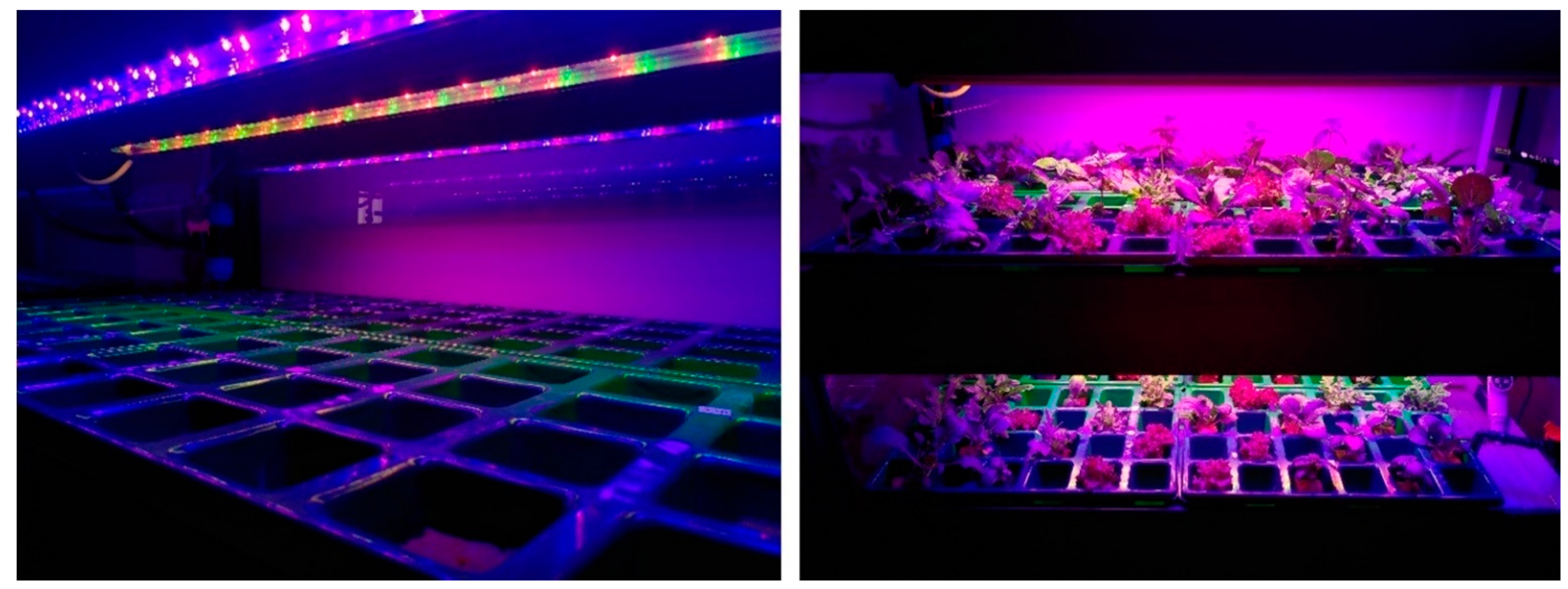
Figure 1.
Smart Office Farm (Photos: Farmee GmbH, 2020 (left) and Cichocki, 2020 (right)).

Figure 2.
LED units and planting trays (left) and an overview of PL about two weeks after germination (right) (Photos: Cichocki, 2020).
Figure 2.
LED units and planting trays (left) and an overview of PL about two weeks after germination (right) (Photos: Cichocki, 2020).

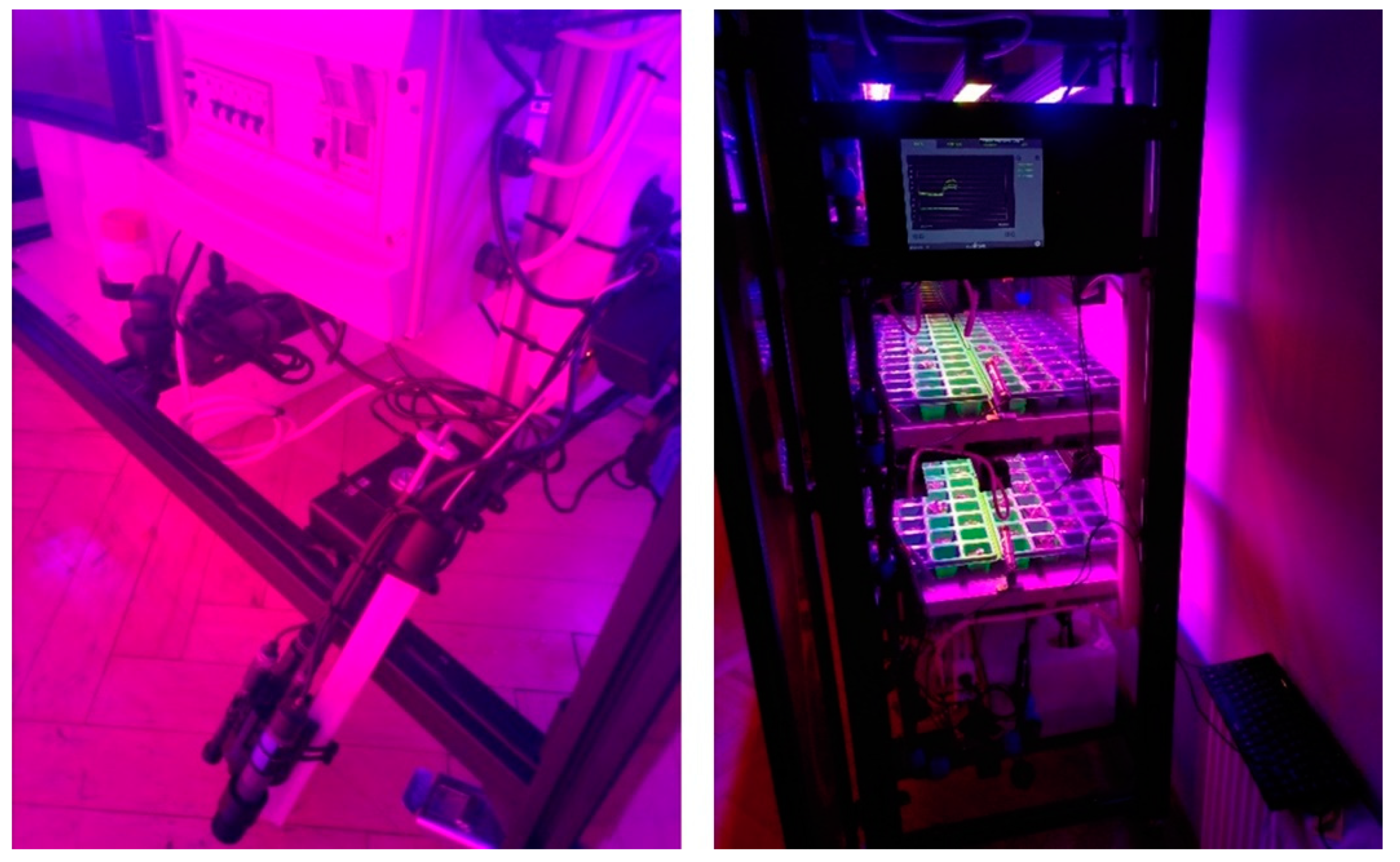
Figure 3.
Monitoring unit, sensors for temperature, humidity, pH, EC and the irrigation control cabinet (left) and the user interface (right) (Photos: Cichocki 2020).
Figure 3.
Monitoring unit, sensors for temperature, humidity, pH, EC and the irrigation control cabinet (left) and the user interface (right) (Photos: Cichocki 2020).

Figure 4.
Photosynthetic photon flux density (PPFD) distribution at production level (µmol m−2 s−1).
Figure 4.
Photosynthetic photon flux density (PPFD) distribution at production level (µmol m−2 s−1).

Figure 5.
Planting plan of the production levels based on a randomized block design with three photosynthetic photon flux density (PPFD) level: 185.2 µmol m−2 s−1 (blue); 355.7 µmol m−2 s−1 (orange); 466.4 µmol m−2 s−1 (grey). Every square represents one planting space (Curled: Curled lettuce, Lolo: lolo rosso, Pak: pak choi and Basil: basil).

Figure 6.
Overview of the material flow and production cost assessment, summarizing all inputs on the left side and all outputs on the right side (extrapolated values) (Photo: Winkler 2020).
Figure 6.
Overview of the material flow and production cost assessment, summarizing all inputs on the left side and all outputs on the right side (extrapolated values) (Photo: Winkler 2020).

Figure 7.
SOF inputs: weekly cumulated water consumption over 35 days.

Figure 8.
Dry matter (DM) yield of the crops under different photosynthetic photon flux density (PPFD) levels.
Figure 8.
Dry matter (DM) yield of the crops under different photosynthetic photon flux density (PPFD) levels.

Figure 9.
Fresh matter yield of the crops under different production levels and photosynthetic photon flux density (PPFD) levels.
Figure 9.
Fresh matter yield of the crops under different production levels and photosynthetic photon flux density (PPFD) levels.

Figure 10.
Comparison of yield; Mean World (red); field conditions (green); greenhouse (blue); SOF (orange); vertical farming companies (green).
Figure 10.
Comparison of yield; Mean World (red); field conditions (green); greenhouse (blue); SOF (orange); vertical farming companies (green).

Figure 11.
Energy consumption per kg of biomass SOF (blue), and vertical farm (orange) (adapted from [14]).
Figure 11.
Energy consumption per kg of biomass SOF (blue), and vertical farm (orange) (adapted from [14]).


Table 1.
Three blocks with three different PPFD and DLI.
| Mean | PPFD (µmol m−2 s−1) | DLI (mol m−2 d−1) |
|---|---|---|
| Block 1 | 185.19 | 10.6 |
| Block 2 | 355.69 | 20.5 |
| Block 3 | 466.44 | 26.6 |
| Total | 335.77 | 19.3 |
Table 2.
Overview of the SOF inputs (number of crops and seeds).
| Plant | Seed Usage | Price (EUR) |
|---|---|---|
| Curled lettuce | 72 | 1.35 |
| Lollo rosso | 72 | 1.35 |
| Pak choi | 72 | 0.60 |
| Basil | 120 | 0.95 |
| Total | 4.24 |
Table 3.
SOF inputs: Overview of types, amounts and costs of the fertilizers used in this study.
| Fertilizer | Costs (EUR L−1) | Usage (mL) | Price (EUR) |
|---|---|---|---|
| Remo ‘grow’ | 13.30 | 45 | 0.60 |
| Remo ‘magnifical’ | 19.86 | 45 | 0.89 |
| Remo ‘Micro’ | 19.85 | 45 | 0.89 |
| Total | 2.39 |
Table 4.
SOF inputs: Overview of types, amounts and dosages of nutrients applied in this study [28].
Table 4.
SOF inputs: Overview of types, amounts and dosages of nutrients applied in this study [28].
| Element | (mg Trial−1) | (g m−2) |
|---|---|---|
| Nitrogen (N) | 2337.1 | 2.947 |
| Phosphorus (P) | 615.4 | 0.776 |
| Potassium (K) | 1680.3 | 2.119 |
| Magnesium (Mg) | 1552.5 | 1.958 |
| Calcium (Ca) | 3375.0 | 4.256 |
| Boron (B) | 27.0 | 0.034 |
| Copper (Cu) | 33.8 | 0.043 |
| Iron (Fe) | 681.8 | 0.860 |
| Manganese (Mn) | 67.5 | 0.085 |
| Molybdenum (Mo) | 0.3 | 0.0004 |
| Zinc (Zn) | 33.8 | 0.043 |
Table 5.
SOF inputs: pH-buffer used in this study and their implied costs.
| pH-Buffer | Usage (mL) | Costs (EUR L−1) | Price (EUR) |
|---|---|---|---|
| pH down | 103.06 | 20.90 | 2.15 |
| pH up | 11.16 | 8.90 | 0.10 |
| Total | 2.25 |
Table 6.
SOF inputs: application dates, amounts and costs of irrigation.
| Date | Water Usage (L) | Costs (EUR L−1) |
|---|---|---|
| 08.07.20 | 36 | 0.003 |
| 15.07.20 | 7.92 | 0.003 |
| 22.07.20 | 11.88 | 0.003 |
| 29.07.20 | 15.48 | 0.003 |
| 05.08.20 | 33.12 | 0.003 |
| 12.08.20 | 38.88 | 0.003 |
| Total | 143.28 | 0.29 |
Table 7.
Total yield of the crops investigated in this study.
| Crop | Yield (g) |
|---|---|
| Curled lettuce | 517.9 |
| Lollo rosso | 403.4 |
| Pak choi | 676.8 |
| Basil | 363.8 |
| Total | 1961.8 |
Table 8.
Yield per PL and PPFD block.
| Block | Crop | Yield PL 1 | Yield PL 2 |
|---|---|---|---|
| Block 1 (Low PPFD) | [g FM] | [g FM] | |
| Curled lettuce | 48.2 | 52.1 | |
| Lolo rosso | 30.4 | 42.2 | |
| Pak choi | 52.5 | 76.8 | |
| Basil | 24.1 | 36.0 | |
| Block 2 (Intermediate PPFD) | Curled lettuce | 45.3 | 73.2 |
| Lolo rosso | 33.9 | 57.7 | |
| Pak choi | 69.8 | 105.9 | |
| Basil | 32.0 | 54.6 | |
| Block 3 (High PPFD) | Curled lettuce | 43.1 | 83.3 |
| Lolo rosso | 43.7 | 61.0 | |
| Pak choi | 65.3 | 80.8 | |
| Basil | 42.0 | 53.8 | |
| Total (2 PL) | 530.3 | 777.5 |
Table 9.
Results of two-tailed paired t-test (p < 0.05).
| PL 1 | PL 2 | |
|---|---|---|
| Mean | 44.19 | 64.80 |
| Variance | 186.05 | 390.27 |
| Observations | 12 | 12 |
| Pearson Correlation | 0.86 | |
| df | 11 | |
| t Stat | −6.69 | |
| P (T ≤ t) two-tail | 3.42 × 10⁻⁵ | |
| t Critical two-tail | 2.20 |
Table 10.
Scenario analysis: Calculated productivity of the individual crop.
| Scenario | Crop | Yield (g) | Yield (g m−2) |
|---|---|---|---|
| 1 | Curled lettuce | 2071.4 | 2612.1 |
| 2 | Lolo rosso | 1613.5 | 2034.7 |
| 3 | Pak choi | 2707.0 | 3413.7 |
| 4 | Basil | 1455.2 | 1835.1 |
Table 11.
Scenario analysis: Productivity in g m−2 5 weeks−1 and Mg FM ha−1 year−1.
| Scenario | Productivity during Observation Period (g m−2 5 Weeks−1) | Calculated Annual Productivity (Mg FM ha−1 Year−1) |
|---|---|---|
| 1 | 2612.1 | 272 |
| 2 | 2034.7 | 212 |
| 3 | 3413.7 | 355 |
| 4 | 1835.0 | 191 |
| Mixed | 2473.9 | 257 |
Table 12.
Economical assessment (renewable energy mix): production factors, costs and their relative contribution to the total costs.
Table 12.
Economical assessment (renewable energy mix): production factors, costs and their relative contribution to the total costs.
| Production Factors | Costs (EUR) | Share of Total Costs (%) |
|---|---|---|
| Electricity | 74.9 | 71.8 |
| Substrate | 15.5 | 14.8 |
| Seeds | 6.4 | 6.1 |
| Fertilizer | 3.6 | 3.4 |
| pH-buffer | 3.4 | 3.2 |
| Water | 0.3 | 0.6 |
| Total | 104.3 | 100 |
Table 13.
Economical assessment (conventional energy mix): production factors, costs and their relative contribution to the total costs.
Table 13.
Economical assessment (conventional energy mix): production factors, costs and their relative contribution to the total costs.
| Production Factors | Costs (EUR) | Share of Total Costs (%) |
|---|---|---|
| Electricity | 79.1 | 73.1 |
| Substrate | 15.5 | 14.3 |
| Seeds | 6.4 | 5.9 |
| Fertilizer | 3.6 | 3.3 |
| pH-buffer | 3.4 | 3.1 |
| Water | 0.3 | 0.3 |
| Total | 108.2 | 100 |
Publisher’s Note: MDPI stays neutral with regard to jurisdictional claims in published maps and institutional affiliations. |
© 2022 by the authors. Licensee MDPI, Basel, Switzerland. This article is an open access article distributed under the terms and conditions of the Creative Commons Attribution (CC BY) license (https://creativecommons.org/licenses/by/4.0/).
Share and Cite
MDPI and ACS Style
Cichocki, J.; von Cossel, M.; Winkler, B. Techno-Economic Assessment of an Office-Based Indoor Farming Unit. Agronomy 2022, 12, 3182. https://doi.org/10.3390/agronomy12123182
AMA Style
Cichocki J, von Cossel M, Winkler B. Techno-Economic Assessment of an Office-Based Indoor Farming Unit. Agronomy. 2022; 12(12):3182. https://doi.org/10.3390/agronomy12123182
Chicago/Turabian StyleCichocki, Jedrzej, Moritz von Cossel, and Bastian Winkler. 2022. "Techno-Economic Assessment of an Office-Based Indoor Farming Unit" Agronomy 12, no. 12: 3182. https://doi.org/10.3390/agronomy12123182
Note that from the first issue of 2016, this journal uses article numbers instead of page numbers. See further details here.