TreeMerge: A Visual Comparative Analysis Method for Food Classification Tree in Pesticide Residue Maximum Limit Standards

Abstract

Food classification is an important part of food safety standards. In this paper, we propose a novel visual comparative analysis method for food classification trees (FCTs) in pesticide maximum residue limit (MRL) standards, called TreeMerge, to lay the foundation for a comprehensive comparison of pesticide MRL standards. First, a union tree is constructed by combining the two FCTs to be compared. Then, sunburst with an embedded chordal graph (SECG) and overlapping circular treemap (OCT), which are two new visualization solutions designed in this paper, are used to show the similarities and differences in a union tree. SECG can express the hierarchical structure and the similarity between corresponding nodes in the union tree at the same time. OCT uses an improved nested Venn diagram (overlapping circle) to express the attribute values in each layer of the union tree and uses a circle-filling layout algorithm based on the testing circle to improve the readability and space utilization of the view. Finally, a visual analysis system for comparing FCT, named FCTvis, is designed and implemented to support the exploration of the structural difference pattern of food classification in the two MRL standards and the quantity or scale of residue limits in various foods. The effectiveness of TreeMerge was verified by case studies on pesticide MRL standards in the Chinese Mainland and Chinese Hong Kong.

1. Introduction

Pesticide residues are one of the major contributors to food safety issues [1,2]. Pesticide maximum residue limit (MRL) standards specify the legally allowed maximum limits of pesticides in food or agricultural products [3]. MRL standards, to a certain extent, reflect the level of management of pesticide residues in agricultural products in a country or region. MRL standards may vary from country to country or region to region. The number of food and pesticide species, the number and limit values of pesticide limits in food, and the food classification system may be greatly different. For example, GB2763-2016 [3] formulated by the Chinese Mainland contains 433 pesticides and 4140 MRL values of these 433 pesticides in various agricultural products. The Regulation on Pesticide Residues in Food [4] formulated by Chinese Hong Kong, contains 360 pesticides and 7083 MRL values of these 360 pesticides in various agricultural products. Their food classification systems are also different. For example, “Banana” belongs to the “Large fruit” food group in the standard of Chinese Mainland, while it belongs to the “Peel inedible tropical and subtropical fruits” food group in the standard of Chinese Hong Kong, as shown in Figure 1.

An analysis of the differences between the MRL standards in different countries or regions is not only conducive to promoting the improvement of their own standards but also beneficial to the food import and export trade between countries. The food classification system is an important part of the MRL standard. It is also the basis for finding the pesticide MRL values in the MRL standard. Comparing the food classification of different countries or regions can help food enterprises (especially export food enterprises) quickly grasp the food category to which their products belong in the export destination and then find out the MRL values of pesticides in the MRL standards of the exporting countries. It can also track the development of MRL standards over time to improve their own standards. It can be seen that comparing the food classification systems of different countries or regions is an indispensable task to analyze the differences between MRL standards.

The food classification system is a multi-level complex hierarchical structure. In the MRL standard, when the limits of a pesticide are applied to a food category, all foods within that food category should comply with these limits, except for those with special specifications. Therefore, the MRL values have an inherited nature in the food classification system. Considering the hierarchical structure of food classification and the inherited nature of limit values, we define the food classification system as a tree, i.e., the food classification tree (FCT). The node of FCT is food or food classification and the attribute value of the node is the number of MRL values specified in that food or classification. The larger the attribute value of a node is, the more pesticide MRLs are specified in the food or classification. In turn, the problem of comparing and analyzing food classifications in different regions is abstracted into the problem of comparing two FCTs.

The comparison of two FCTs is a complex task because of the hierarchical structure of FCTs and the inherited nature of node attribute values. Traditional manual comparison or comparison methods based on table tools are inefficient, less accurate, and less intuitive. The quantitative tree comparison method based on structural similarity can describe the degree of structural differences between two trees from a macroscopic perspective [5] but describing the details of the differences between two trees is difficult. Visual analytics (VA) is the science of analytical reasoning based on visual interactive interfaces [6], which maps complex data into easy-to-understand visual representations such as graphs, symbols, and colors, supplemented by interactive means, to enhance humans’ understanding and analysis of data and thus quickly discover features and patterns hidden within the data [7]. VA has achieved good results in many fields and has started to be applied to solve tree comparison problems [8,9,10,11,12,13]. In recent years, researchers have proposed a series of visual analysis methods for tree comparison, such as juxtaposition, merging, and animation, and have achieved better results.

However, due to the specificity of FCT, the existing tree comparison visual analysis method still has the following problems: (1) Discovering the pattern of structural differences between two FCTs is difficult. Existing methods usually use node similarity metrics to quantify the overall degree of structural differences in the subtree rooted at these two nodes and the positions of all nodes in the subtree to show the details of structural differences between these two nodes. However, by applying this approach, users can compare only a small number of nodes in the subtree at a time and cannot simultaneously show the pattern of structural differences of all nodes in the subtree, i.e., the pattern of structural differences of the two root nodes to be compared, e.g., all corresponding nodes in the two subtrees have completely different or identical structures. (2) Visually comparing and analyzing the differences in the structure and node attribute values of two FCTs at the same time and exploring the effects of structural differences on node attribute values is difficult. The existing methods analyze the structural differences and attribute value differences independently of each other, i.e., they try to analyze the attribute value differences with small or no topological structure differences, and the topological structure differences are analyzed with minimal consideration of the attribute value differences. The node attribute values of FCT are closely related to food classification, and the influence of FCT structure differences on node attribute values needs to be considered. Therefore, correlation analysis of structural differences and node attribute value differences is needed, which is a new challenge.

In this paper, we propose TreeMerge, a novel method for visual comparative analysis of FCTs in pesticide MRL standards. It helps users visually compare and analyze the similarities and differences in topology and node attributes between two FCTs and explore the effects of structural differences on attribute values. We also designed and implemented a food classification comparison visual analysis system called FCTvis based on the above method. The main contributions of this paper are as follows:

(1)

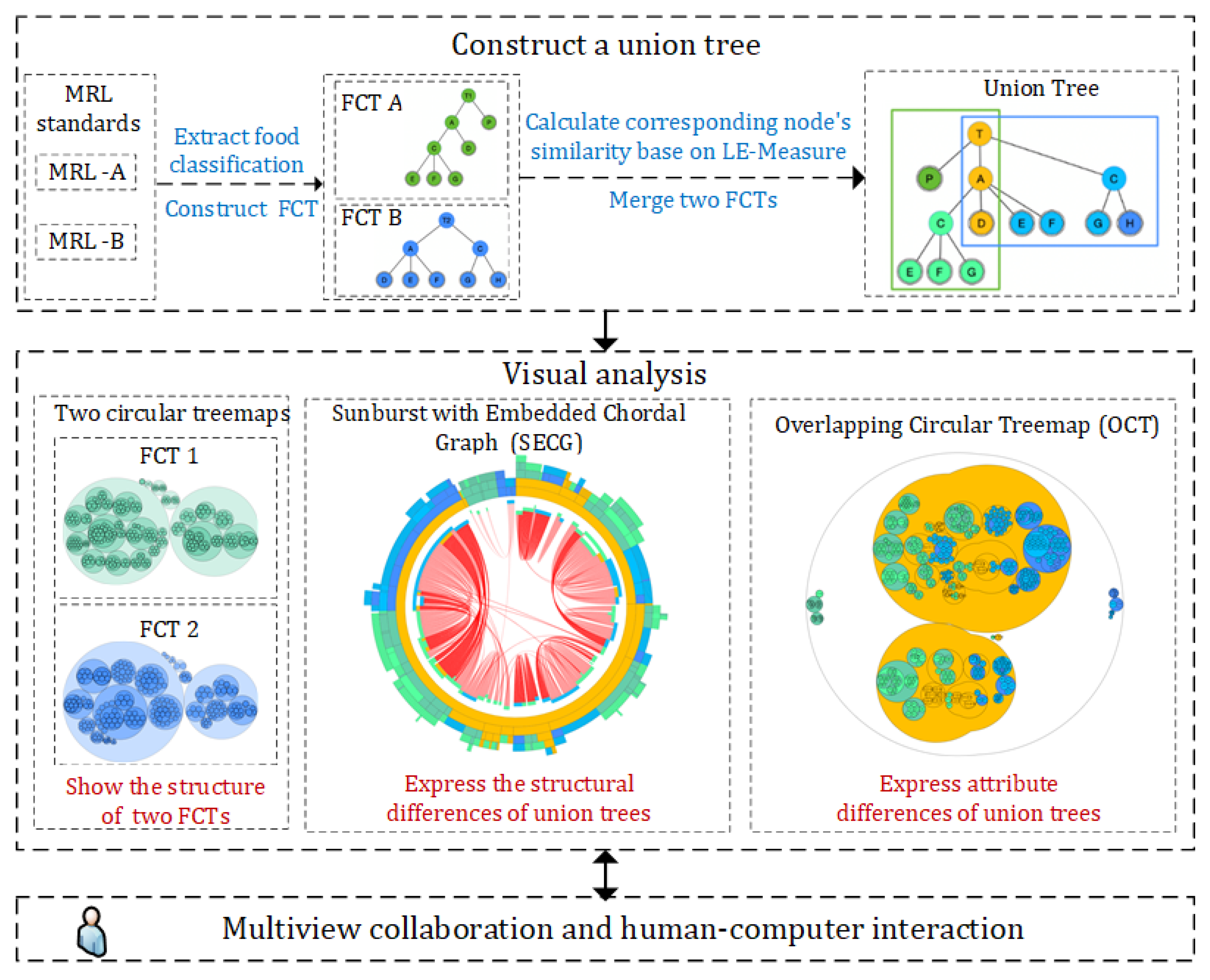
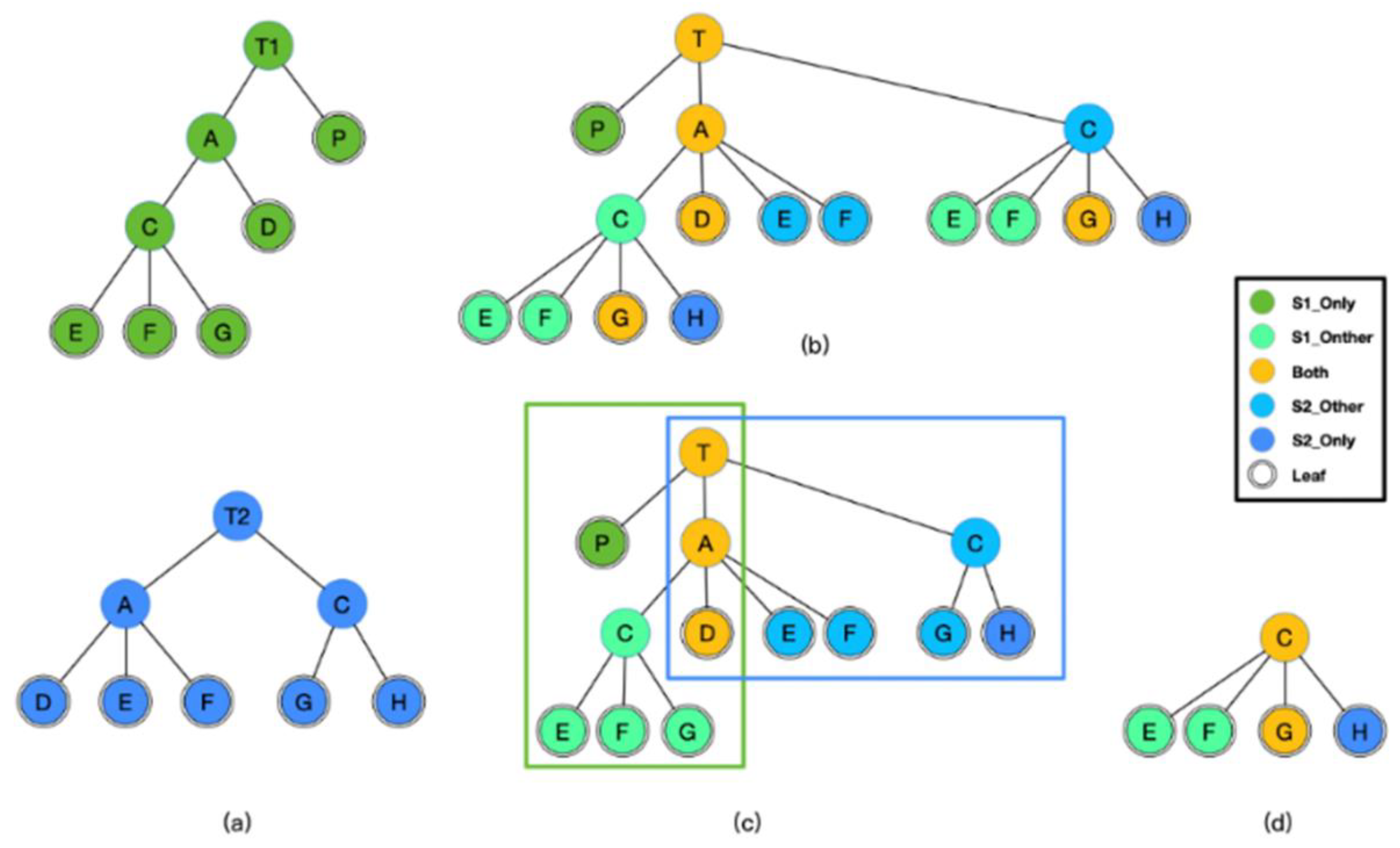
A union tree construction method is proposed, which merges two FCTs into a single union tree based on the improved node similarity metric LE-Measure in this paper. The union tree provides the basis for a visual associative representation of the structural and attribute differences between the two FCTs to be compared.

(2)

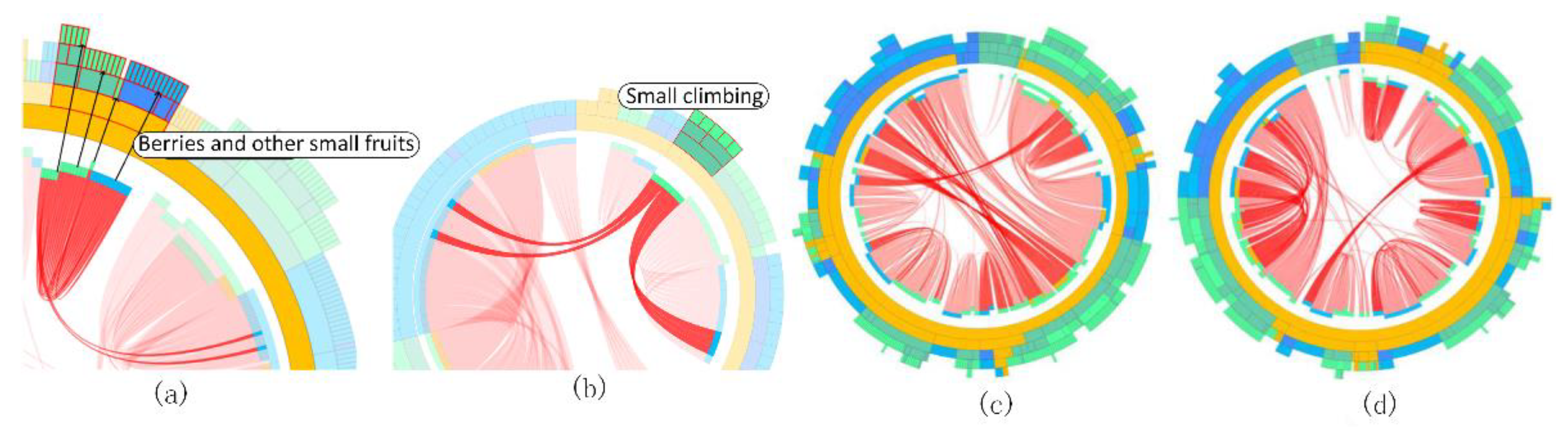
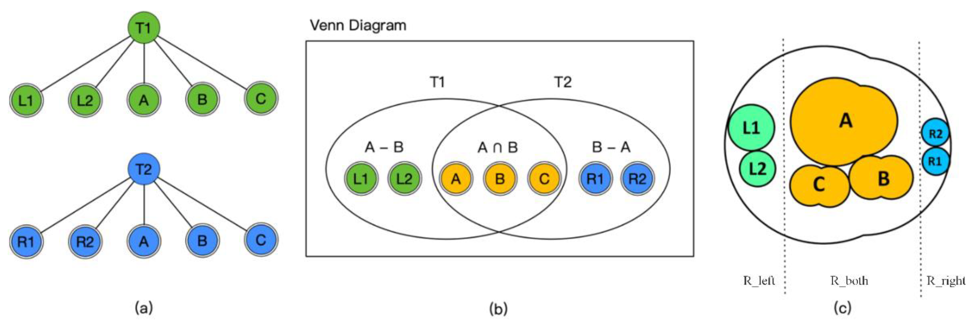
Two new visualization solutions called sunburst with an embedded chordal graph (SECG) and the overlapping circular treemap (OCT) are proposed to visualize the similarities and differences between two trees to be compared contained in a union tree. They support the exploration of the structural difference pattern of food classification in the two regions and realize the correlation analysis of food classification and the number of residue limits in food or food classification.

(3)

A visual analysis system for comprising food classification trees, FCTvis, is designed and implemented. Case studies were conducted on the pesticide MRL standards in the Chinese Mainland and Chinese Hong Kong to verify the effectiveness of the TreeMerge method.

2. Related Work

2.1. Tree Comparison Visualization

Methods for tree comparison visualization can be divided into three categories: Juxtaposition, merging, and animation.

Juxtaposition means placing two or more trees side by side for comparison. Many tree comparison visualization methods use juxtaposition to show structural differences between hierarchies. Chevalier et al. proposed CodeFlow, which integrates structural information from the C++ source code into a tree structure and visually connects the same part of the tree structure [14]. Holten et al. enhanced the display of differences by concatenating nodes in two trees and adding edge-binding techniques [15]. Bremm et al. used a matrix as an overview of the differences between any two trees in a multi-tree comparison. After the tree is selected for comparison, the nodes in the tree are juxtaposed with the nodes in the reference tree for a comparison of differences, and the corresponding nodes and edges in the tree are mapped using the same color to facilitate user comparison [16]. Liu et al. designed and implemented the ADView system, which merged multiple trees and then juxtaposed them for comparison to solve the visual comparison of multiple phylogenetic trees occurring in evolutionary biology, especially between a reference tree and a collection of tens to hundreds of other trees [17]. Chen et al. used a circular treemap to represent the trees and juxtaposed two trees to compare them through a coordinated analysis of multiple views [18]. Li et al. represented each tree with a barcode to achieve space reduction and then juxtaposed multiple trees to compare multiple trees simultaneously [9].

Merging refers to the merging of two trees into a collection tree. To improve spatial efficiency, some have proposed merging the trees to be compared [19,20,21,22,23,24], preserving the complete structure and attribute information of both trees, and visually comparing the collection tree visualization by using node linking or space filling. Leschke et al. proposed Change-Link 2.0 to analyze the differences in document structure over time, where leaf nodes are color and shape coded in the TreeView view, and color-coded segments correspond to time periods when the corresponding directory does not yet exist (yellow), does exist (green), and used to exist but has been removed (orange) [25]. Lee et al. used merged trees to compare hierarchical structures, referred to changes in the structure as uncertainty, and used cadidTree to visualize uncertainty in the directory structure [23]. TreeVersity2 encoded changes in node attributes using color, height, and shape and represented these differences in a hierarchical view [21]. Recently, Fu et al. combined sankey and treemap designs to implement TreeEvo for statistical analysis of a large number of tree structures and proposed the concept of propensity to describe the imbalance in the development of descendants in genealogical trees [26].

Animation methods are usually used to compare data with time-varying features and to observe the changes of nodes in different tree structures by switching between animations [27]. For example, the TimeTree designed by Card et al. switched the tree structure at different times by dragging the time axis [28]. However, the change in node positions usually makes the comparison more difficult.

Juxtaposition is suitable for structure comparison, which can visually find similar parts in the structure. However, when the similarity of two trees is high, a large number of identical structures will appear on both sides at the same time, and users need to switch their views frequently. Using the merged approach to compare two trees, the merged structure of two trees can show the pattern of different structures more clearly than the juxtaposition approach. Thus, we merge two trees and compare the topology and attribute values of the two trees.

2.2. Circle Packing

The circular treemap, which was first proposed in 1991 [29], is a special use of Venn diagrams because only the containment relations are used in it as opposed to multiple set relation representations of Venn diagrams. As a special type of treemap, it recursively divides circular regions into multiple sub-circles based on the data structure. The circular treemap can clearly display hierarchical structures with a single aspect ratio, and it can be used for datasets with hierarchically structured data [30]. Gou et al. designed TreeNetViz using radial space filling visualization to represent the tree structure, a novel optimized circular layout to display aggregation networks derived from TreeNet, and edge-bundling techniques to reduce visual complexity [31]. Jochen et al. presented a novel type of circular treemap, which introduced a hierarchical and force-based circle-packing algorithm to compute bubble treemaps, where each node was visualized using nested contour arcs [32]. Zhao et al. proposed variational circular treemaps. They divided the weights for each node in the hierarchical data and defined the disk-packing algorithm to traverse the nodes in a top-down manner to achieve the layout of circular tree graphs [33]. Wang et al. designed a bottom-up layout approach, which we used in our layout design [34].

The circle packing problem concerns placing a set of circles in a container without overlap and finding the smallest container by combinatorial optimization. The most classical packing problem is packing N (N = 1, 2, …) equal circles in a circle. Huang et al. solved this problem by modeling two motions of each disk [35]. Birgin et al. proposed a nonlinear model for containers of different shapes within 2D and 3D [36]. For the problem of scheduling non-equally sized circles, Huang et al. proposed two new heuristic algorithms [37]. Zhao et al. used a power diagram to implement a global optimal scheduling method [33].

In this paper, the visualization design not only pursues the tightness of sub-node arrangement and higher space utilization but also pays attention to the balance between view readability and space utilization.

3. Dataset and Analysis Task

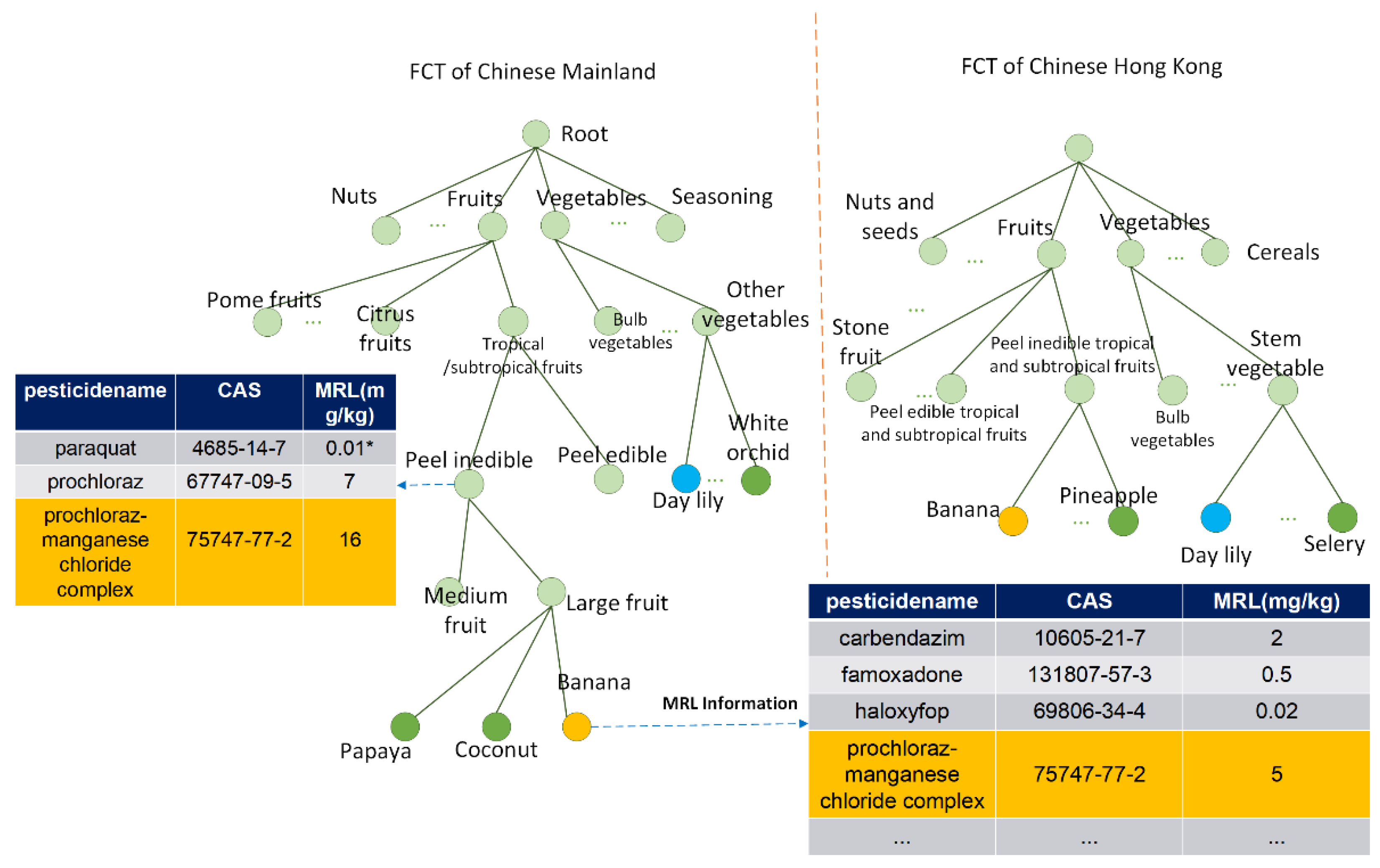
3.1. Dataset and FCT

The dataset used in this paper is part of the standards of GB2763-2016 formulated by the Chinese Mainland and the Pesticide Residues in Food Regulation formulated by Chinese Hong Kong [3,4]. The dataset contains MRLs for 433 pesticides in 241 agricultural products and food categories at all levels in the Chinese Mainland, totaling 4140 items, and MRLs for 360 pesticides in 227 agricultural products and food categories at all levels in Chinese Hong Kong, totaling 5760 items. The FCTs of the two regions are shown in Figure 1, and the label of the node is the name of the food or food category represented by the node.

The data characteristics of the two FCTs are shown in Figure 2. Figure 2a shows the distribution statistics of the number of nodes in each depth for the two FCTs in the Chinese Mainland and Chinese Hong Kong. We can see (1) the leaf nodes in the two trees are randomly distributed at different depths and not “normatively” distributed at the deepest depth; (2) the number of nodes at the same depth in the two trees is not the same, and the ratio of leaf nodes to internal nodes varies significantly. In traditional tree comparison visualization methods, both features are difficult to deal with, increasing the mapping difficulty and understanding the cost of tree comparison visualization. In Figure 2b, (1) yellow represents the number of nodes with matching labels and also matching positions (i.e., the same name and the same classification of the same food) between the two trees; (2) dark green and dark blue represent the number of nodes in the first tree and the second tree that each exist independently (i.e., different foods or different names of the same food); (3) light green and light blue represent the number of nodes with matching labels but not matching paths between the two trees (i.e., same name but a different classifications of the same food). As can be seen from Figure 2b, the two regions have very few perfectly matched food classifications, and the classification differences have a certain generality.

The nodes in the FCT carry MRLs. A MRL contains the limit value of a pesticide in the food or food classification node, i.e., each node contains multiple MRLs. Figure 1 shows the MRLs carried by the “Banana” and “Peel inedible tropical and subtropical fruits” nodes in the FCT of the Chinese Mainland. Nodes in FCT inherit MRLs from their parent classification nodes, and leaf nodes inherit their own undefined MRLs from their ancestor nodes in their paths (except for special exemptions). Therefore, the differences in MRLs carried by foods in different MRL standards are largely due to their classification differences, in addition to the different limit values defined by the nodes themselves.

$$\mathrm{M}\left({\mathrm{C}}_{\mathrm{p}}^{\mathrm{j}}\right)= \mathrm{M}\left(\mathrm{P}\right)\cup \mathrm{M}\left({\mathrm{C}}_{\mathrm{p}}^{\mathrm{j}}\right)$$

(1)

For the child node ${\mathrm{C}}_{\mathrm{p}}^{\mathrm{j}}$ of node P (j is the child node serial number), which itself carries the MRLs expressed as $\mathrm{M}\left({\mathrm{C}}_{\mathrm{P}}^{\mathrm{j}}\right)$, each MRL is expressed as a binary group of p = (S, L). S is the name of the pesticide and L is the pesticide residue limit value. Starting from the root node, the MRLs of all nodes are updated by substituting Equation (1) from top to bottom in turn. For example, “Peel inedible tropical and subtropical fruits” in Figure 1 itself carries MRLs M (“Peel inedible tropical and subtropical fruits”) = {p1, p2, p3}, where p3 = (“Prochloraz-Manganese chloride complex”, 16). The node “Large fruit” and the node “Coconut” themselves carry 0 MRLs. Thus, the node “Coconut” will inherit the MRLs of the parent node, M(“Coconut”) = {p1, p2, p3, …}, where p3 = (“prochloraz-manganese chloride complex”, 16). As can be seen from Figure 1, the sub-node “Banana” of “Large fruit” also specifies the pesticide limits for “prochloraz-manganese chloride complex” and other pesticide limits, so M(“Banana”) = {p1, p2, p3, p4, p5, …}, where p3 = (“prochloraz-manganese chloride complex”, 5). The quantity of MRLs ${\mathrm{V}}_{\mathrm{p}}^{\mathrm{j}}=|\mathrm{M}({\mathrm{C}}_{\mathrm{p}}^{\mathrm{j}})|$ carried by the node ${\mathrm{C}}_{\mathrm{p}}^{\mathrm{j}}$ is the attribute value of ${\mathrm{C}}_{\mathrm{p}}^{\mathrm{j}}$, i.e., the quantity or scale of residue limits in various foods is used as the node attribute value.

3.2. Analysis Tasks

Based on the complex hierarchical characteristics of the dataset, the universality of food classification differences, and the inherited nature of MRLs, the following target analysis tasks are developed for the food classification comparison between the two regions.

Task 1. Analysis of path differences of individual nodes. Because of the inherited nature of node attributes in FCTs, it may be necessary to find the MRLs of ancestral classification nodes in the tree when analyzing the MRLs of a specific classification or agricultural product node. In addition to the MRLs possessed by the nodes themselves, path differences are the main reason for the differences in node attributes.

Task 2. Global hierarchical ordered overview. A clear hierarchical display can effectively locate structural differences and visually compare the addition, deletion, and movement of nodes in two trees. Combined with node similarity analysis, the node pairs with analytical value or interest can be quickly located, which is the key work of visual analysis.

Task 3. Analysis of details and patterns of structural differences. Design appropriate visualization schemes to describe the details of structural differences, patterns of structural differences, and nested representations of patterns of structural differences in the descendant hierarchy.

Task 4. Effect of topology differences on attribute change. The comparison of MRL standards under the same structure can be regarded as the comparison of nodes’ attributes, but the influence of topological differences should be considered under different structures. Thus, it helps experts further analyze MRL standard differences in terms of differences in food classification.

3.3. Pipeline of TreeMerge

Based on the above analysis task, this paper proposes a novel visual comparative analysis method called TreeMerge for FCTs in pesticide MRL standards, and the pipeline of TreeMerge is shown in Figure 3. (1) First, we construct a union tree and extract food classifications from two MRL standards, respectively, to build two FCTs. Based on the improved node similarity metric, LE-Measure, we calculate the corresponding node similarity of the two trees, merge the two FCTs to be compared, and construct a union tree to express the similarities and differences in the structure and attributes of the two FCTs. (2) A visual analysis is carried out, in which two circular treemaps are used to show the structure of the two FCTs to be compared. We design a visualization solution, SECG, to show the structural difference information embedded in the union tree, and design another visualization solution, OCT, to show the attribute differences in the union tree. (3) Lastly, we design interaction techniques to achieve multi-view collaboration and human–computer interaction.

4. Union Tree

4.1. Definitions of Labeled Tree

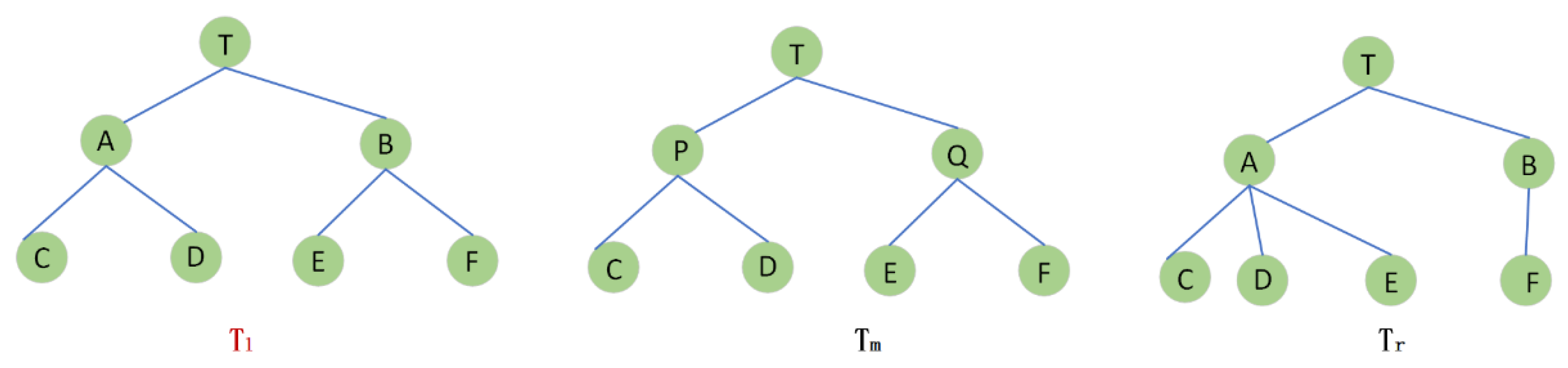
A rooted FCT T with all nodes labeled is called a labeled tree. Labeled tree T = (V, E) contains a set of undirected edges E that connect a pair of labeled parent–child nodes. For two compared labeled trees ${\mathrm{T}}_1$ and ${\mathrm{T}}_2$, if two nodes in ${\mathrm{T}}_1$ and ${\mathrm{T}}_2$ have the same label, then they are called a pair of shared nodes. Conversely, unique nodes on ${\mathrm{T}}_1$ or ${\mathrm{T}}_2$ are called unique nodes. A path in a tree is defined as a unique sequence of connected nodes p(${\mathrm{n}}_1$, ${\mathrm{n}}_{\mathrm{k}}$) = ${\mathrm{n}}_1$, ${\mathrm{n}}_2$, …, ${\mathrm{n}}_{\mathrm{k}}$ where ${\mathrm{n}}_{\mathrm{i}}$∈V and (${\mathrm{n}}_{\mathrm{i}}$, ${\mathrm{n}}_{\mathrm{i}+1}$)∈E. Shared nodes with different paths are called moved nodes and represent the nodes that need to be moved when the two trees are transformed into each other.

4.2. LE-Measure

In order to find out the nodes with comparative significance in the two trees, this paper improves the similarity metric of nodes and defines two kinds of node association relations: Explicit and implicit. Explicitly related nodes refer to two nodes with matching labels and the highest similarity to each other, and implicitly related refers to nodes with different labels but the highest similarity to each other.

Node similarity refers to the degree of structural similarity of the subtree rooted at the node to be compared. In previous studies, node similarity was based on the RF distance [38,39] and its variants. Bremm et al. further proposed the Element-base measure, which adds topology to the similarity calculation [16]. However, this measure using only the set of leaf nodes is not sufficient to describe the label matching of internal nodes. Based on this approach, we further take inner node labels into consideration. A novel scoring scheme called LE-Measure, which can distinguish between topology and label mismatches, is designed to compare two rooted trees with labelled inner nodes. The degree of similarity in the subtree structure of ${\mathrm{T}}_1$ and ${\mathrm{T}}_2$ is defined as

$${\mathrm{s}}_{\mathrm{l}}\left({\mathrm{T}}_1, {\mathrm{T}}_2\right)=\frac{\left|\mathrm{LE}\left({\mathrm{T}}_1\right)\cap \mathrm{LE}\left({\mathrm{T}}_2\right)\right|}{\left|\mathrm{LE}\left({\mathrm{T}}_1\right)\cup \mathrm{LE}\left({\mathrm{T}}_2\right)\right|}$$

(2)

We define the label-element score of a tree ${\mathrm{T}}_{\mathrm{i}}$ as

$$\mathrm{LE}\left({\mathrm{T}}_{\mathrm{i}}\right)=\left\{\left\{\mathrm{L}\left({\mathrm{T}}_{\mathrm{i}}^{\mathrm{n}}\right)\right\},\forall {\mathrm{n}}_{\mathrm{i}}\in {\mathrm{T}}_{\mathrm{i}}\right\}\}\cup \mathrm{A}\left({\mathrm{T}}_{\mathrm{i}}\right)$$

(3)

The set of all leaf nodes of a tree ${\mathrm{T}}_{\mathrm{i}}$ is denoted as L(${\mathrm{T}}_{\mathrm{i}}$), and a subtree ${\mathrm{T}}_{\mathrm{i}}^{\mathrm{n}}$∈${\mathrm{T}}_{\mathrm{i}}$ is a tree consisting of a node n∈${\mathrm{T}}_{\mathrm{i}}$ and all of its descendants in ${\mathrm{T}}_{\mathrm{i}}$, while $\mathrm{LE}\left({\mathrm{T}}_{\mathrm{i}}\right)$ means to obtain all the leaf nodes of the subtree of the tree ${\mathrm{T}}_{\mathrm{i}}$ whose descendant node 𝑛 is the root node. The set of all nodes (including the root node) of a tree ${\mathrm{T}}_{\mathrm{i}}$ is A(${\mathrm{T}}_{\mathrm{i}}$). The similarity between ${\mathrm{T}}_1$ and ${\mathrm{T}}_2$ is defined as ${\mathrm{s}}_{\mathrm{l}}\left({\mathrm{T}}_1,{\mathrm{T}}_2\right)$ with 0 ≤ ${ \mathrm{s}}_{\mathrm{l}}$≤ 1.

The two common label differences are shown in Figure 4. Tree ${\mathrm{T}}_{\mathrm{m}}$ has the same structure and leaf nodes as tree ${\mathrm{T}}_{\mathrm{l}}$, but different internal node labels. Tree ${\mathrm{T}}_{\mathrm{r}}$ has only the same internal node labels (except the root node) as tree ${\mathrm{T}}_{\mathrm{l}}$. Tree ${\mathrm{T}}_{\mathrm{l}}$ and tree ${\mathrm{T}}_{\mathrm{m}}$ in Figure 4 are taken as an example, $\mathrm{LE}\left({\mathrm{T}}_{\mathrm{l}}\right)=\left\{\mathrm{T}, \mathrm{A}, \mathrm{B}, \mathrm{C}, \mathrm{D}, \mathrm{E}, \mathrm{F}, \left[\mathrm{C}, \mathrm{D}\right], \left[\mathrm{E}, \mathrm{F}\right]\right\}$, and $\mathrm{LE}\left({\mathrm{T}}_{\mathrm{m}}\right)=\left\{\mathrm{T}, \mathrm{P}, \mathrm{Q}, \mathrm{C}, \mathrm{D}, \mathrm{E}, \mathrm{F}, \left[\mathrm{C}, \mathrm{D}\right], \left[\mathrm{E}, \mathrm{F}\right]\right\}$, ${\mathrm{s}}_{\mathrm{l}}\left({\mathrm{T}}_{\mathrm{l}}, {\mathrm{T}}_{\mathrm{m}}\right)=7/11\approx 0.64$.

4.3. Construction of the Union Tree

In this paper, two FCTs are merged to construct a union tree to express the similarities and differences in the structure and attributes of the two FCTs to be compared. The construction of the union tree is a top-down process that recursively constructs child nodes from the root node. The set of children of the root node in both trees is calculated to determine the type of children, and then the union tree of the root node and its children is constructed based on the original position of the node in the two FCTs and the node type. This construction process is performed recursively for each child node, ending when the leaf node is reached. The nodes in the union tree are called merged nodes, and their attributes depend on the attributes of their original nodes. The color mapping of the five different node types is shown in Figure 5, which shows whether the corresponding original nodes exist in both trees and the change in their positions in the two trees.

As shown in Figure 5, the child nodes of T in the union tree are {A, P, C}. In the current layer, we can obtain the set of children nodes of T nodes in the two trees. First, we can obtain the set of child nodes that currently only appear on the first tree, and those that only appear on the second tree, as well as those that exist on both trees. If nodes are exclusive on one tree, then we set their type as S1_Only (or S2_Only); in the case of moved nodes, we set their type as S1_Other (or S2_Other); otherwise, we set their type as Both. Consequently, the types of P, C, and A are S1_Only, S2_Other, and Both, respectively.

However, there are a large number of redundant nodes and structures (Figure 5d) in the union tree constructed based on the above method (Figure 5b). During the construction of the union tree, we need to calculate the similarity between nodes based on LE-Measure, save the node pairs with explicitly related and implicitly related relationships, merge the two subtrees rooted with the corresponding nodes that are explicitly related or implicitly related, and perform pruning operations on the generated new structure in real time. For example, when constructing the subtree of moved nodes, the set of child nodes will correspond to the structure of the original tree, and the nodes of both attributes will be changed to S1_Other and S2_Other, respectively, as shown in Figure 5c for the two G nodes. The final constructed union tree is shown in Figure 5c.

5. Visualization Design

5.1. Sunburst with Embedded Chordal Graph Design

Sunburst with an embedded chordal graph (SECG) is an overview visual design of a union tree. As shown in Figure 6, the outer part of SECG is sunburst, which maps all merged nodes and their hierarchical relationships, and the color maps the nodes’ type. In sunburst, the innermost ring represents the division of food categories, and the classification level increases from the inside to the outside and the food categories become more and more detailed. The value represented by the area size of each ring block can reflect the percentage of each food node or classification node in that level. The inner side of SECG uses a chord diagram to describe the correlation between nodes in the union tree. The principle is to connect two related nodes by curves. The starting and ending nodes of the inner curve and the corresponding nodes of the outer sunburst are mirror-symmetric of the innermost circle of the sunburst. The transparency of the curves can be used to map hierarchical information (in the default and explicitly related views, the deeper the connected nodes are, the darker the color) or similarity information (in the implicitly related view, the closer the similarity is to 1, the darker the color).

As shown in Figure 6a, for the “Berries and other small fruits” node in the Chinese Mainland, the red border highlights the structure of its descendants, and the inner curves show the node pairs of its descendants related to the FCT of Chinese Hong Kong. We have marked some of the external sunburst nodes with black arrows to show the correspondence with the inside curve start or end nodes. From Figure 6a,b, we can find that the light-colored and yellow nodes have a mirror relationship, and a curve connecting another node must be present.

The inner region of SECG is often used to express the movement trend of all descendants of two merged nodes. In the inside mapping area, the relative positions between the nodes remain unchanged, and the associated nodes are connected using the curve, while the beginning and end of the curve are dependent on the level of the node, so users can easily find the mapping position between the inside and the outside. As shown in Figure 6c,d, the layout of all child nodes of one node will be sorted according to the node type: Both, S1_Only, S1_Other, S2_Other, and S2_Only. This arrangement allows the curves to be more aggregated and ensures that the related node pairs in the node descendants are positioned as close to each other as possible, i.e., the starting and ending positions of the curves corresponding to the inner part of the SECG will be relatively close. The closer the common ancestor of two associated nodes is to the root node, the closer the curve is to a straight line. Otherwise, the curve is more curved and a set of nodes with the same ancestor will produce an effect similar to edge binding. Therefore, by observing the distribution state of the curves to find the key associated nodes, it is the main method for experts to explore the structural differences.

The interaction in SECG consists of a toggle button, mouse over, and mouse click. Toggle button: Button switching is used to switch different types of curves inside. Mouse over: When the mouse passes a node outside, the inside will highlight the curve connected to these matched nodes. Mouse click: For left-clicking, focus and context are provided by clicking inner nodes. For right-clicking, the diagram will highlight the path of the two associated nodes with their paths outside and display the movement of the descendant inside by highlighting all related curves.

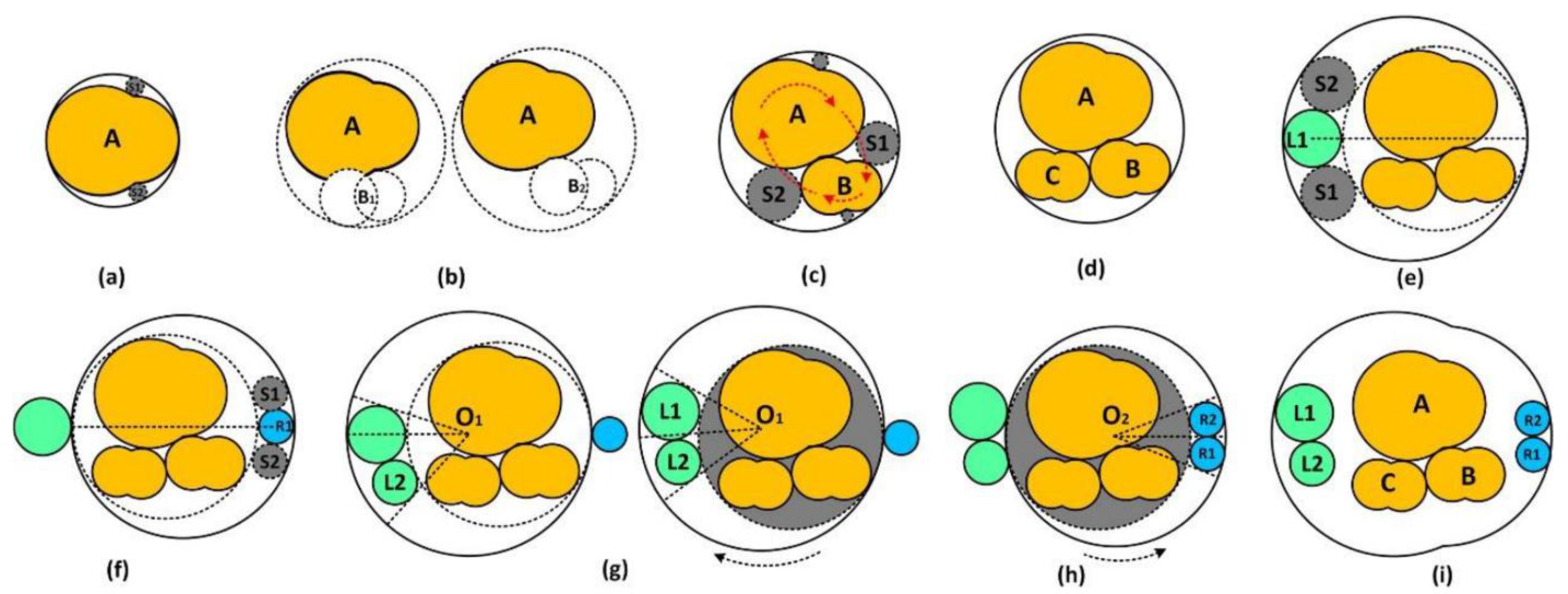
5.2. Overlapping Circular Treemap Design

This chapter will initially depict the shape mapping of the parent and the layout algorithm of its child in OCT, and then construct the entirety of OCT.

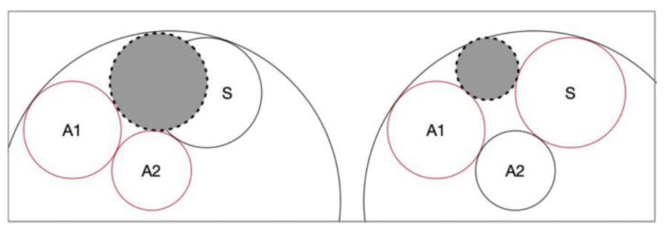
5.2.1. Node Shape Mapping

The shape of the nodes in the union tree is improved from a circle to a shape similar to a Venn diagram, called an overlapping circle. An overlapping circle is a shape formed by two circles that completely or partially overlap for mapping merged nodes. The degree of overlap of the node descendant structure is expressed by an analogy with the overlapping parts of the Venn diagram. As shown in Figure 7, the merged node T is the merger of T1 and T2 in Figure 7a. The design of the overlapping circles corresponding to the union tree of trees T1 and T2 is shown in Figure 7c, similar to the Venn diagram shown in Figure 7b, where R_left, R_both, and R_right are equivalent to the left, middle, and right positions of the Venn diagram. The overlapping circle position indicates the type of the child node, the size of the child node is determined by its property value, and the shape of the parent node depends on the layout result of the child node. The nodes in the R_left and R_right regions have only one value that represents the quantity or scale of residue limits for that food or that food category in different regions. The nodes in the R_both region have three attribute values, the numbers on the left and right represent the attribute values of the node in the two FCTs, noted as v1 and v2, and the middle value represents the number of two regional standards that are identical, noted as v_both (in this paper, agricultural products or classification nodes carry MRL, if the “pesticide name” and “pesticide maximum residue limit value” are equal at the same time to be considered the same item).

In this paper, we propose the concept of propensity to measure which of a pair of descendant subtrees of two trees has a more independent structure or larger attribute values, mapping the propensity of nodes in terms of the size of the shape of the overlapping circle left and right, i.e., the region represented by the side with the larger overlapping circle shape has a larger scale of MRL standard regarding that food classification.

5.2.2. Child Set Layout

The layout process of child nodes in Figure 7c is demonstrated in Figure 8. Child nodes in S1 and S2 are placed in the overlapping circle’s R_left region and R_right region, and those in Both are in the R_both regions. The nodes in each of the three regions are sorted by attribute value in descending order (for nodes in the Both set, they can be sorted by the sum of the attribute values of the two nodes) and placed in order.

While placing the largest node (overlapping circles) in the R_both regions, the sequence of overlapping circles that are closest to the outer major circle, i.e., the smallest outer circle of all the current overlapping circles, is traversed (in the order of the red arrows in Figure 8c) and all testing circles (gray circles in Figure 8c) are calculated using Equation (4). The possible placement positions are detected based on the testing circles, and the optimal placement position of the next overlapping circle, i.e., the position where the largest testing circle is located, is calculated (Figure 8d). The next overlapping circle is placed at the optimal position, the new external circles and sequence are calculated, and the optimal placement position of the next node is calculated in turn. Figure 8b shows the process of detecting possible placement positions based on testing circles: First, we try to place testing circles to detect whether there is overlap with the already placed overlapping circles. Then, we select the placement level position without overlap (as shown in Figure 9).

$$\begin{array}{c}{\left(\mathrm{x}-{\mathrm{x}}_1\right)}^2+{\left(\mathrm{y}-{\mathrm{y}}_1\right)}^2={\left(\mathrm{r}\pm {\mathrm{r}}_1\right)}^2\\ {\left(\mathrm{x}-{\mathrm{x}}_2\right)}^2+{\left(\mathrm{y}-{\mathrm{y}}_2\right)}^2={\left(\mathrm{r}\pm {\mathrm{r}}_2\right)}^2\\ {\left(\mathrm{x}-{\mathrm{x}}_3\right)}^2+{\left(\mathrm{y}-{\mathrm{y}}_3\right)}^2={\left(\mathrm{r}\pm {\mathrm{r}}_3\right)}^2\end{array}$$

(4)

where ${\mathrm{x}}_1$, ${\mathrm{y}}_1$, ${\mathrm{r}}_1,$ and ${\mathrm{x}}_2$, ${\mathrm{y}}_2$, ${\mathrm{r}}_2$ refer to the coordinate of the circle center and the radius of two adjacently placed circles (one overlapping circle is considered two circles), ${\mathrm{x}}_3$, ${\mathrm{y}}_3$, and ${\mathrm{r}}_3$ are the center coordinate and radius of the circumcircle, and the value of ${\mathrm{r}}_3$ is negative.

After all nodes in the R_both regions are placed, the large circle of R_both is used as the central location to place the nodes on both sides. The nodes on both sides, as shown in Figure 8e–h, are placed staggered left and right. First, the largest node in the R_left region is placed horizontally with the circles of R_both, as shown in Figure 8e, and the initial circles and sequences of this region are generated. Then, all the testing circles are calculated to find the appropriate position of the next node, and the circles and sequences are updated (the same for the right R region as in Figure 8f). For each new node placed, the overlapping circles that are already placed are rotated to remain relatively horizontal (Figure 8g). When all the nodes on both sides are placed, the overlapping circle consisting of the outer circles on both sides is the shape of the parent node (Figure 8i).

5.2.3. Construction of the Entire OCT

The shape of the parent node depends on its children, so the whole OCT construction process requires a bottom-up approach, as follows: The leaf nodes in the union tree are mapped to the corresponding overlapping circles based on the improved nested Venn diagram, and then the optimal placement of the overlapping circles is calculated using the above circle-filling layout algorithm based on the testing circles, and the layout of the overlapping circles is completed recursively from the bottom up to construct the shape of the parent node, until the shape of the root node is constructed. The node attributes v1 and v2 are the radii of the two circles in the overlapping circle, and v_both is the distance between the centers of the two circles.

The structure difference pattern of the two nodes to be compared refers to the structure difference pattern of all nodes in the subtree using these two nodes as roots. In this paper, several typical structural difference patterns are summarized by the shape of the parent nodes in the OCT and the distribution of blue and green nodes in its child node set, as shown in Figure 10. The most common ones are (a) the common structure, where identical and discrepant parts are present in the offspring; (b) the isomorphic structure, where the parent node is circular because the node has exactly the same set of children as the corresponding node in the union tree, and therefore the overlapping circles completely overlap; (c) the separate structure, which is due to the complete absence of identical nodes in the set of children of a node that has a related relationship; and (d) the contained structure, which is also a completely separated state, but because the set of children of one of the related nodes is a subset of the other.

The overlapping circle shape allows an intuitive propensity analysis, and the distribution state of the child nodes indicates the reason for shape separation. The shape of the parent node is so sensitive that the overlapping circles are separated even if only one blue or green node is present. Therefore, the blue and green nodes on both sides are the focus of the analysis. Globally, the denser the distribution of these two types of color nodes, the greater the corresponding classification differences. Locally, light-colored nodes correspond to a set of moving nodes.

The interaction in OCT consists of toggle button, mouse over, and mouse click. Mouse over: When the mouse is close to one shared node, the corresponding node is also marked, and the size of the circles represents the attribute values. Mouse click: Left click provides the “focus-context” interaction. Toggle buttons: The first three buttons enable OCT view movement, display node labels, and display node attributes, while the last button enables aggregation mode. In aggregation mode, the hierarchical information present in the descendants is discarded, and the focus is on how the values of the node attributes differ from each other. All shared nodes are combined and displayed at the same level, leaving aside nodes that cannot be matched in the current subtree or independent nodes.

5.3. SECG-OCT Interactive

We use circular treemap, SECG, and OCT to compare trees in terms of structure and attribute value differences. The interaction means of “context-detail” linkage analysis is realized by combining the respective advantages of SECG and OCT views. The interaction is designed as follows.

In the SECG view, the mouse hovers over a node and the corresponding node and its hierarchical information in the OCT view are highlighted with a red border. By right clicking on the node in the light green, light blue, or yellow area of sunburst outside the SECG view and using the red line in the external area of SECG to highlight the path or subtree topology of the selected node, only the property information of the selected node and its sub-nodes is displayed in the OCT view. Similarly, right clicking on a node in the OCT view will highlight the topology of the selected node’s path or subtree using a red line in the external area of the SECG. All nodes are displayed in the OCT, but the selected node and its children are highlighted.

6. FCTvis System

6.1. FCTvis Interface

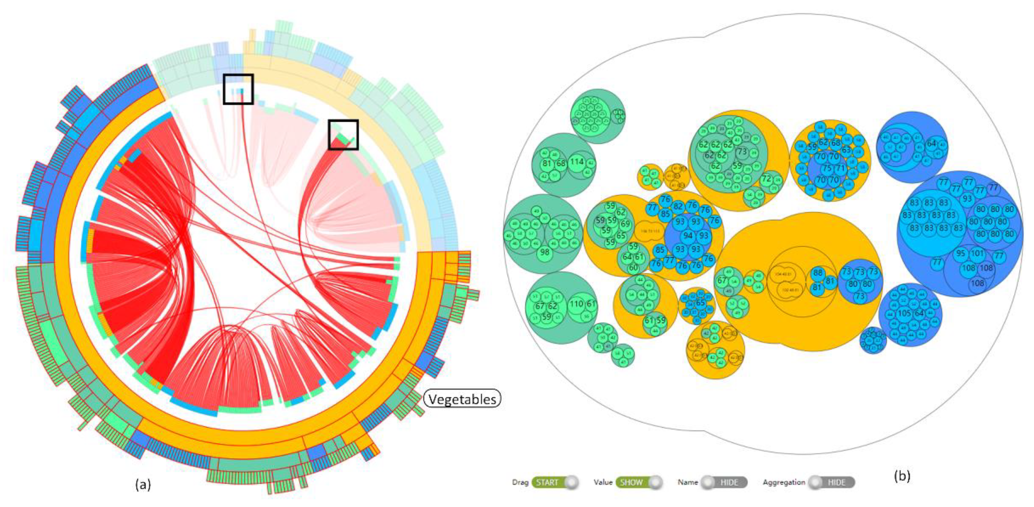
On the basis of the above methods, an FCT visual comparison analysis system FCTvis was designed and implemented. The main interface of the system is shown in Figure 11.

(a)

The two circular treemaps are visual mappings of the two FCTs to be compared, and the histograms show the statistical information of the nodes on the different levels. In the circular treemap, when the mouse hovers over a node in a tree, the node and its descendant structure are highlighted. If the node is related to a node in another tree, then the corresponding structure in the other tree is also highlighted. This interaction is a juxtaposition of comparisons and is used to prompt the user. When the mouse clicks on an internal node, the SECG view displays information about that node only, facilitating further observation of the local structure. The circular treemap can also be associated to show the structural information of the selected nodes of the SECG view and the OCT view.

(b)

The SECG view is used to provide a visual overview of the structural differences. By default, it displays structural information about the root node descendants of the union tree constructed with all food products and the related relationships between the descendant nodes. Mouse hovering will highlight the curve between this node and the related nodes internally, and the node label will be displayed externally. The SECG view displays the descendant structure information of the selected node when the left mouse button is clicked on the internal node in Figure 11a or on the dark green, dark blue, or yellow area in the external sunburst in the SECG view. The type of node pairs connected by internal curves can be changed via the toggle button. By default, curves that connect two identically labeled leaf nodes are displayed. Clicking the toggle button above will display curves that connect explicitly related internal node pairs. Clicking the toggle button below allows SECG to display curves that connect implicitly related node pairs.

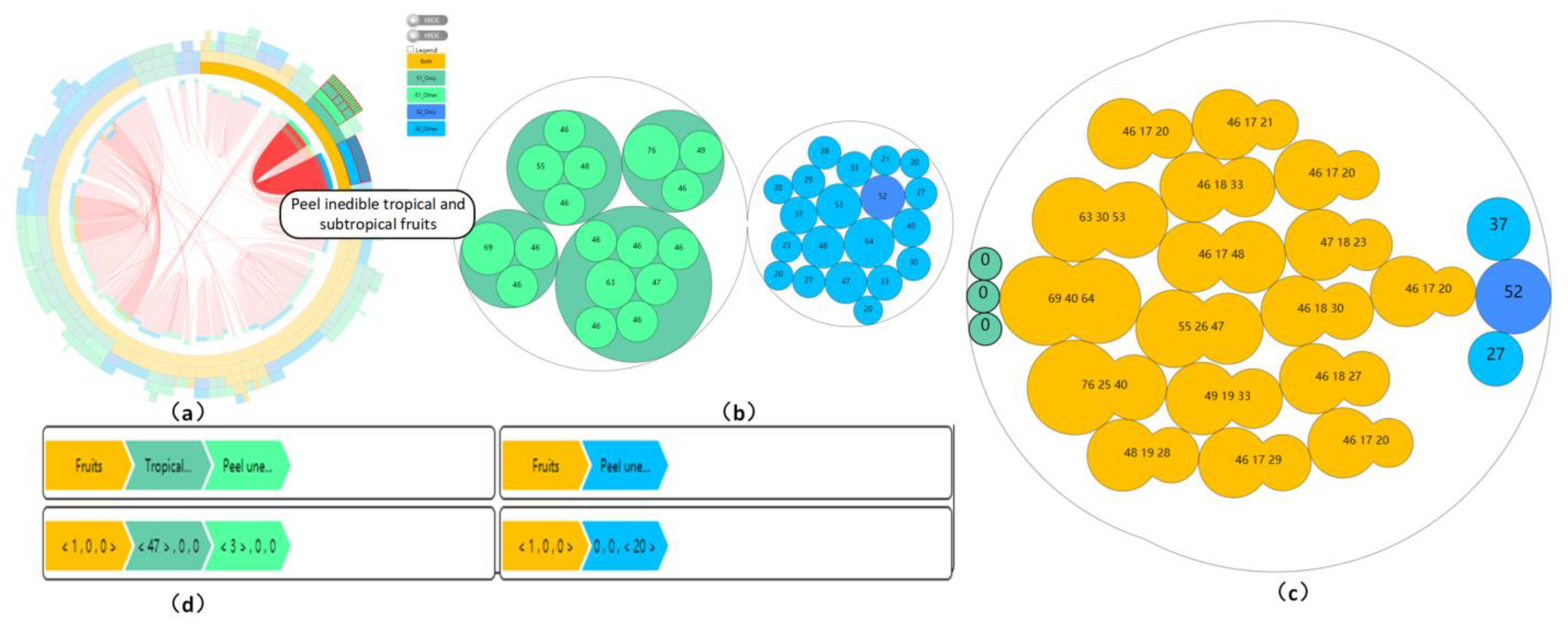
(c)

This is used to show the path of the selected node in Figure 11b and the changes in the node value attributes in that path, i.e., it is used to show the complete genetic process of the MRL of the selected node. Each node has three values: The value of the leaf node corresponds to its attribute value in different FCT trees according to the color of the node; the value in the middle region of the attribute value of the internal node, i.e., the food classification node, represents the number of the same MRL value inherited by the present selected node under the two classifications; and the values on both sides correspond to the number of MRL value related to this classification node inherited by the selected node in the two FCTs, respectively.

(d)

The OCT view is used for the visual mapping of structural difference patterns and node attribute values. The OCT view by default displays the union tree built with all food products. Left clicking on a node in the middle area of the overlapping circle or a blank area is used to drill down and scroll up the data, i.e., switch the nodes displayed in the OCT view. Using the given button, we can lock the current view position, display node attribute values, display node labels, and switch the aggregation mode. Clicking the right mouse button can be linked with the circular treemap and the SECG view in Figure 11a to compensate for topological information that cannot be displayed by OCT.

6.2. Case Study

To verify the effectiveness of the FCTvis, we invited experts from relevant fields and experts from the field of visualization to test it. In the beginning, we explained the entire process of the system for 20 min to help the experts become familiar with the system, then left 40 min for free exploration. This section describes the overall process of the expert application system and the conclusions. We denote the visualization experts as E0, E1, and E2 and the MRL experts as E3, E4, and E5.

6.2.1. Topology Discovery by the SECG Overview

E1 praised the SECG view for providing a tight, clear display of the hierarchy and commented that the structure of the two trees is highly distinguishable by mapping the colors of the merged nodes (Task 2). The union tree with yellow node elements on the outside of the SECG decreases layer by layer, i.e., the same structure in the two FCTs becomes less and less as the hierarchy goes deeper and deeper. When nodes of other colors appear in the yellow node subtree, it means that the structure is unique to a certain tree, which can help users locate the classification differences.

E0 proposed that SECG provides overall topological information with information on the distribution trend of node movement, but adding attribute mapping would cause information overload, which is well addressed by linkage with OCT. OCT is used not only to map differences in attribute values of individual leaf nodes but also to show local structural differences. However, OCT has limitations in mapping a specific node, as describing moved nodes that are not in the current subtree is not possible. For example, the green moved nodes in the box cannot be mapped to the “Vegetables” node in Figure 12b, but E0 can find them through the curves in Figure 12a, i.e., the curves of SECG provide location retrieval for these nodes.

In response to the need to analyze the path difference analysis of individual nodes (Task 1), E3 determined the distribution of moved nodes by observing the light-colored nodes in the external region of the SECG and hovered over these light-colored nodes to view the specific movement status of that food or food category’s descendant nodes, i.e., the classification difference of the same food product in the two FCTs, through Figure 11c. Moreover, the quantity or scale of residue limits in various food can be viewed through Figure 11c, and the number of limits that are identical as well as different can be visually compared between similar or homonymous node pairs. Figure 12a shows the classification differences between the food products of the two regions under the observation of the “Vegetables” classification, where the curves are visually clearly constrained into groups according to their span, which represents the topicality of the movement of the descendant nodes, i.e., most of the nodes are well constrained in a few substructures. E3 believed that this indicates a high degree of commonality in the classification of the two regions, which provides a good overview of the corresponding food products.

E3 is interested in the path differences between nodes with related relationships and the topological changes of the descendants of these nodes. Thus, when he hovered over the node “Peel inedible tropical and subtropical fruits” based on the color of the node in the external area of SECG, the highlighted curve directed him to another corresponding node (Figure 13a). By right-clicking, the two paths of these nodes are highlighted in the outer area. Furthermore, the process of passing and accumulating the leaf nodes according to the path properties is shown (Figure 13d). The external region of the SECG then uses red borders to highlight the topology of the subtrees of these nodes (as in Figure 13a). The aggregation structure of the two subtrees is visualized as an OCT (Figure 13b). The attribute differences can be further explored by switching to the aggregation mode (Figure 13c).

Experts are interested in curves with small curvature and discrete endpoints that represent node pairs with large differences in classification in two regions. Experts explored the impact of these node pair path differences on node attributes by combining the attribute values of the nodes in the OCT view. For example, the analysis revealed that the “Leek flower” is classified as a “Herb” in Chinese Hong Kong and as “Vegetables” in the Chinese Mainland. An exploration of the attribute value transfer process of “Leek flower” shows that in the Chinese Mainland, it involves 44 standards, but it does not define any standards itself and inherits almost all of them from the standards of “Bulb vegetables”. In Chinese Hong Kong, it involves 13 standards, all of which are defined by itself and are completely different from those in the Chinese Mainland.

6.2.2. Attribute Detail Analysis

E2 right-clicked the “Vegetables” node in the SECG view and observed the details of the differences in the descendant structures of the “Vegetables” node in the OCT view, the patterns of structural differences, and the nested expressions of the patterns of structural differences in the descendant hierarchy (Task 3). Figure 12b shows that the local structure difference pattern of the “Vegetables” node is a common pattern, in which Chinese Hong Kong has a more unique classification structure than the Chinese Mainland, which is related to the complex structure of the independent classification “Fruit vegetables” in Chinese Hong Kong. Finally, among the sub-nodes in the common part, several typical patterns of structural differences in offspring can be quickly found based on the shape of the current node: “Aquatic vegetables” with isomorphic patterns, “Leafy vegetables” and “Bulb vegetables” with segregate patterns, and “Bud vegetables” with contained patterns. (Task 3)

In the process of analyzing the effect of structural differences on attributes (Task 4), E5 observed the shape of nodes in OCT, analyzed the propensity of nodes, and quickly selected several advantageous classifications of Chinese Mainland FCT with more complex topologies: “Fruits”, “Leafy vegetables”, “Bulb vegetables”, “Berries and other small fruits”, etc. In the same way, she identified advantages in a few classifications in the FCT of Chinese Hong Kong: “Vegetables”, “Melons”, “Citrus fruits”, etc. E5 left-clicked on these nodes in turn, made the OCT view focus on the current node, and observed the tendency details of the children and intermediate nodes on both sides, to understand the status of their independent topologies and common topologies, respectively. She then used the aggregation mode to check the attribute differences of the descendants. She said the shape of the leaf nodes aptly describes the difference in MRLs held by the food in two regions, i.e., for a given node in a nested Venn diagram, if the circular curve on the left side of the Venn diagram is larger, it means that the left FCT has more detailed limits developed for that node than the right FCT. E5 continued to view the attributes on the basis of topology difference patterns (Task 3) and used the aggregation mode to visualize the differences in attribute values. As a result, she found that in a few classifications inclined to the FCT of the Chinese Mainland, there is always a more detailed classification of the food products under the same category. However, these refined sub-categories do not carry MRLs by themselves. Thus, in the aggregation mode, these sub-categories have a node value of 0 and typical cases such as the node, “Peel inedible tropical and subtropical fruits”, “Leafy vegetables”, and “Bulb vegetables”, etc. E5 believes that such a feature may provide a direction to improve the Chinese Mainland’s MRL standards, which was not noticed in the previous comparative analysis of MRL standards.

The nodes with implicit correlation can be indexed by the curves provided by SECG, for example, “Melon fruits” in the FCT of the Chinese Mainland and “Melons” in the FCT of Chinese Hong Kong. Although the two categories have great path differences, the descendant structures are very similar. E4 examined the MRLs of these food products using the aggregation mode, and they also have a high degree of similarity. Examining the respective paths revealed that the two classifications themselves have a high overlap of MRLs, while their respective offspring do not have many MRLs. Therefore, they both rely on inherited MRLs from both classifications, thus maintaining the consistency of attributes. The same situation occurred in “Legume vegetables”, “Pod vegetables”, “Root and taro vegetables”, and “Root and potato vegetables”. E4 considered these examples to be tautological, and although the labels of the nodes are different, and the locations of the nodes differ significantly, the path differences do not have a significant impact on the attribute values, and the attribute values can be directly compared in their descendants.

While exploring the topology using SECG, E3 noticed that several special curves with large differences in curvature appear in the same set of curves. This type of curve is unlikely to occur in correlated pairs of nodes. This phenomenon is more common in independent classifications (where nodes are not related), and nodes with related offspring are often distributed in multiple classifications in another tree, resulting in a set of curves with many branches. Food products under independent classifications often have large differences in attributes, depending on whether multiple classifications in another region provide different MRLs. For example, “Fruit vegetables” in the FCT of Chinese Hong Kong belongs to “Edible mushrooms” and “Eggplant and fruit vegetables” in the FCT of the Chinese Mainland. Obviously, the “Edible mushrooms” category does not provide MRLs in the Chinese Mainland, while the “Fruit and vegetable” category can provide 70 MRLs. In contrast, the “Fruit and Vegetable” category provides 40 MRLs, while the node itself carries more than 30 MRLs, which is better than the “Fruit and Vegetable” category in Chinese Hong Kong. Another typical example is “Stem vegetables” in Chinese Hong Kong. This is a typical phenomenon of an unbalanced distribution of MRLs due to classification differences.

6.2.3. Case Exploration Process

We tested FCTvis in the context of import/export trade. It is assumed that vegetables from Chinese Hong Kong will be sold to the Chinese Mainland.

The representatives of vegetable companies in Chinese Hong Kong can first find the circle representing the “Chili” node by hovering over it in the circular treemap of Chinese Hong Kong (Figure 11a), and the circle representing the “Chili” node in the circular treemap of the Chinese Mainland will also be highlighted. Then, by exploring the circular treemap of the Chinese Mainland layer by layer, we can clarify the classification of “Chili” in the Chinese Mainland. In addition, we can also click on the classification node in the circular treemap of Chinese Hong Kong, and the SECG view will zoom in to show only the classification information of that node for further observation.

When exporting and sampling the residue limit of a pesticide in “Chili” of “Fruit vegetables” in Chinese Hong Kong, if the MRL standard of the Chinese Mainland does not specify the MRL of this pesticide in “Chili”, we need to first determine which category of vegetables it belongs to. We can use the above approach to query its parent category, which is “Other eggplant”, to determine whether to specify the MRLs of this pesticide, and if not, we can query the MRLs of “Eggplant vegetables” up the hierarchy of queries.

Finally, we can quickly locate the classification differences by observing the node color on the outside of the SMLC and the related nodes by the curves on the inside of the SMLC. We can hover over a vegetable node in the SMLC and view the details of the classification to which this vegetable belongs in both regions, as well as the changes in the quantity and scale of the limits for each level of classification to which it belongs, by using Figure 11c to visually compare the number of identical and different standards for this vegetable. Users can also right-click on the “Vegetables” node in SMLC (Figure 11b) to observe the classification differences and the pattern of structural differences between the two regions under the “Vegetables” category, and the user interface is shown in Figure 12.

As shown above, the system can help representatives of Chinese Hong Kong exporting companies to quickly grasp the food category of various vegetables in the Chinese Mainland and then find the standards and requirements for that food in the Chinese Mainland. Specifically, the method helps representatives of exporting companies to interactively compare the differences and the pattern of structural differences in food classification between MRL standards in Chinese Mainland and Chinese Hong Kong, inquire whether the food to be exported has a corresponding standard in the Chinese Mainland, and compare the number of pesticide residue limit values on the food and analyze how many identical standards on the food are available in the Chinese Mainland and Chinese Hong Kong.

7. Discussion

The experts used the FCTvis system for case studies and discussed the limitations of the visualization design. The experts praised the fact that the linkage between SECG and OCT works very well. Moreover, SECG solves the local limitations in OCT exploration, and OCT provides detailed attribute information to SECG to avoid SECG information overload. The shape mapping of nodes in OCT also provides a reference value for analyzing the advantages and disadvantages of the currently selected set of nodes, i.e., the local MRL standard.

In the process of exploration, the experts also put forward further suggestions. E2 hopes to see a better visual description of the inheritance process of attributes in the path rather than a mere numerical value. E5 said that under the aggregation mode, she expects a new view that removes the MRL inherited from the current classification’s path and simply focuses on the transfer process of the attribute in the subtree. She considers this approach to be fairer.

8. Conclusions and Future Work

This paper proposes a novel visual comparative analysis method called TreeMerge for FCTs in pesticide MRL standards, which supports users in interactively comparing the similarities and differences in the structure and node attributes of FCTs among MRL standards in two countries or regions, exploring the structural difference pattern of food classification in the two MRL standards, analyzing the association between food classification and the quantity or scale of residue limits in various foods, and laying the foundation for later all-round comparison of MRL standards. On this basis, a visual analysis system for food classification comparison, called FCTvis, is implemented to provide an efficient visual analysis tool for domain experts. This method can also be extended to other food safety standards for food classification comparison, providing a scientific basis for food safety decisions.

In the future, we will study the visual comparative analysis method of MRL standards, comparing the differences among MRL standards of two different countries or regions in macro and micro aspects, including the number of pesticide species, the food classification system and the limit value of pesticides in food, etc. In order to help domain experts and other general users become familiar with the use of this system faster, we will design a more user-friendly interface and ways of operating closer to the domain scenario. In addition, we will design real-time interaction suggestions to help users explore the MRL standard step by step.

References

1. Bakirci, G.T.; Acay, D.B.Y.; Bakirci, F.; Otles, S. Pesticide residues in fruits and vegetables from the Aegean region, Turkey. Food Chem. 2014, 160, 379–392. [Google Scholar] [CrossRef] [PubMed]
2. Chen, Y.; Dou, H.F.; Chang, Q.Y.; Fan, C.L. PRIAS: An Intelligent Analysis System for Pesticide Residue Detection Data. Food Saf. Superv. 2022, 11, 780. [Google Scholar]
3. National Health and Family Planning Commission of PRC; The Ministry of Agriculture of the People’s Republic of China. National Food Safety Standard-Maximum Residue Limits for Pesticides in Food; Standards Press: Beijing, China, 2016.
4. Food and Environmental Hygiene Department. Pesticide Residues in Food Regulation; Food and Environmental Hygiene Department: Hong Kong, China, 2014.
5. Chen, Y.H.; Li, J. A tree similarity computation method based on structure feature. Comput. Eng. 2018, 44, 197–201. [Google Scholar]
6. Ward, M.; Grinstein, G.; Keim, D. Interactive Data Visualization: Foundations, Techniques, and Applications, 2nd ed.; A K Peters Ltd.: Natick, MA, USA, 2014. [Google Scholar]
7. Munzner, T. Visualization Analysis and Design; A K Peters/CRC Press: New York, NY, USA, 2014. [Google Scholar]
8. Chen, Y.; Du, X.M.; Yuan, X.R. Ordered Small Multiple Treemaps for Visualizing Time-Varying Hierarchical Pesticide Residue Data. Vis. Comput. 2017, 33, 1073–1084. [Google Scholar] [CrossRef]
9. Li, G.Z.; Zhang, Y.; Dong, Y.; Liang, J.; Zhang, J.S.; Wang, J.S.; McGuffin, M.J.; Yuan, X.R. BarcodeTree: Scalable Comparison of Multiple Hierarchies. IEEE Trans. Vis. Comput. Graph. 2020, 26, 1022–1032. [Google Scholar] [CrossRef]
10. Chen, Y.; Zhang, Q.H.; Guan, Z.L.; Zhao, Y.; Chen, W. GEMvis: A visual analysis method for the comparison and refinement of graph embedding models. Vis. Comput. 2022, 38, 3449–3462. [Google Scholar] [CrossRef]
11. Chen, Y.; LV, C.; Li, Y.; Chen, W.; Ma, K.-L. Ordered matrix representation supporting the visual analysis of associated data. Sci. China Inf. Sci. 2020, 63, 184101. [Google Scholar] [CrossRef]
12. Chen, Y.; Guan, Z.L.; Zhang, R.; Du, X.M.; Wang, Y.H. A Survey on Visualization Approaches for Exploring Association Relationships in Graph Data. J. Vis. 2019, 22, 625–639. [Google Scholar] [CrossRef]
13. Chen, Y.; Zhang, X.Y.; Feng, Y.C.; Liang, J.; Chen, H.Q. Sunburst with Ordered Nodes based on Hierarchical Clustering: A Visual Analyzing Method for Associated Hierarchical Pesticide Residue Data. J. Vis. 2015, 18, 237–254. [Google Scholar] [CrossRef]
14. Chevalier, F.; Auber, D.; Telea, A. Structural analysis and visualization of C++ code evolution using syntax trees. In Proceedings of the ACM International Conference Proceeding Series, Dubrovnik, Croatia, 3–4 September 2007; pp. 90–97. [Google Scholar]
15. Holten, D.; Van Wijk, J.J. Visual comparison of hierarchically organized data. Comput. Graph. Forum. 2018, 27, 759–766. [Google Scholar] [CrossRef]
16. Bremm, S.; Von Landesberger, T.; Hess, M.; Schreck, T.; Weil, P.; Hamacherk, K. Interactive visual comparison of multiple trees. In Proceedings of the IEEE Conference on Visual Analytics Science and Technology, Providence, RI, USA, 23–28 October 2011; Miksch, S., Ed.; IEEE Computer Society Press: Providence, RI, USA, 2011; pp. 31–40. [Google Scholar]
17. Liu, Z.; Zhan, S.H.; Munzner, T. Aggregated Dendrograms for Visual Comparison Between Many Phylogenetic Trees. IEEE Trans. Vis. Comput. Graph. 2019, 2019, 2732–2747. [Google Scholar] [CrossRef] [PubMed] [Green Version]
18. Chen, Y.; Dong, Y.; Sun, Y.H.; Liang, J. A Multi-comparable visual analytic approach for complex hierarchical data. J. Vis. Lang. Comput. 2019, 47, 19–30. [Google Scholar] [CrossRef]
19. Beck, F.; Wiszniewsky, F.; Burch, M.; Diehl, S.; Weiskopf, D. Asymmetric visual hierarchy comparison with nested icicle plots. In Proceedings of the Fourth International Workshop on Euler Diagrams and the First International Workshop on Graph Visualization in Practice Co-Located with Diagrams, Melbourne, Australia, 28 July–1 August 2014; pp. 53–62. [Google Scholar]
20. Dinkla, K.; Westenberg, M.A.; Timmerman, H.; van Hijum, S.A.; van Wijk, J.J. Comparison of multiple weighted hierarchies: Visual analytics for microbe community profiling. Comput. Graph. Forum 2011, 30, 1141–1150. [Google Scholar] [CrossRef]
21. Guerra, G.J.A.; Pack, M.; Plaisant, C.; Shneiderman, B. Visualizing change over time using dynamic hierarchies: Treeversi-ty2 and the stemview. IEEE Trans. Vis. Comput. Graph. 2013, 19, 2566–2575. [Google Scholar] [CrossRef] [PubMed]
22. Guerra-G’omez, J.A.; Buck-Coleman, A.; Plaisant, C.; Shneiderman, B. TreeVersity: Interactive visualizations for comparing two trees with struc-ture and node value changes. In Proceedings of the Conference Design Research Society, Bangkok, Thailand, 1–4 July 2012; Volume 2, pp. 640–653. [Google Scholar]
23. Lee, B.; Robertson, G.G.; Czerwinski, M.; Parr, C.S. CandidTree: Visualizing structural uncertainty in similar hierarchies. Inf. Visu-Alization 2007, 6, 233–246. [Google Scholar] [CrossRef]
24. Tu, Y.; Shen, H.W. Visualizing changes of hierarchical data using treemaps. IEEE Trans. Vis. Comput. Graph. 2007, 13, 1286–1293. [Google Scholar] [CrossRef] [PubMed] [Green Version]
25. Leschke, T.R.; Nicholas, C. Change-link 2.0: A digital forensic tool for visualizing changes to shadow volume data. In Proceedings of the Tenth Workshop on Visualization for Cyber Security, Atlanta, GA, USA, 14 October 2013; pp. 17–24. [Google Scholar]
26. Fu, S.; Dong, H.; Cui, W.; Zhao, J.; Qu, H. How do ancestral traits shape family trees over generations? IEEE TVCG 2018, 24, 205–214. [Google Scholar] [CrossRef]
27. Sankaran, K.; Holmes, S. Interactive Visualization of Hierarchically Structured Data. J. Comput. Graph. Stat. 2018, 27, 553–563. [Google Scholar] [CrossRef]
28. Card, S.K.; Suh, B.; Pendleton, B.; Heer, J.; Bodnar, J.W. TimeTree: Exploring Time Changing Hierarchies. In Proceedings of the IEEE Symposium on Visual Analytics Science & Technology, Baltimore, MD, USA, 31 October–2 November 2006. [Google Scholar]
29. Johnson, B.; Shneiderman, B. Tree-maps: A space-filling approach to the visualization of hierarchical information structures. In Proceedings of the IEEE Conference on Visualization, San Diego, CA, USA, 21–25 October 1991; pp. 284–291. [Google Scholar]
30. Zheng, B.Y.; Sadlo, F.L. On the visualization of hierarchical multivariate data. In Proceedings of the IEEE Pacific Visualization Symposium, Tianjin, China, 19–21 April 2021; pp. 136–145. [Google Scholar]
31. Gou, L.; Zhang, X.L. TreeNetViz: Revealing patterns of networks over tree structures. IEEE Trans. Vis. Comput. Graph. 2011, 17, 2449–2458. [Google Scholar]
32. Görtler, J.; Schulz, C.; Weiskopf, D.; Deussen, O. Bubble Treemaps for Uncertainty Visualization. IEEE Trans. Vis. Comput. Graph. 2017, 24, 719–728. [Google Scholar] [CrossRef]
33. Zhao, H.S.; Lu, L. Variational circular treemaps for interactive visualization of hierarchical data. In Proceedings of the IEEE Pacific Visualization Symposium, Hangzhou, China, 14–17 April 2015; pp. 81–85. [Google Scholar]
34. Wang, W.X.; Wang, H.; Dai, G.Z.; Wang, H.G. Visualization of large hierarchical data by circle packing. In Proceedings of the SIGCHI Conference on Human Factors in Computing Systems, Montréal, QU, Canada, 22–27 April 2006; ACM Press: New York, NY, USA, 2006; pp. 517–520. [Google Scholar]
35. Huang, W.Q.; Ye, T. Global optimization method for finding dense packings of equal circles in a circle. Eur. J. Oper. Res. 2011, 210, 474–481. [Google Scholar] [CrossRef]
36. Birgin, E.G.; Sobral, F.N.C. Minimizing the object dimensions in circle and sphere packing problems. Comput. Oper. Res. 2008, 35, 2357–2375. [Google Scholar] [CrossRef]
37. Huang, W.Q.; Li, Y.; Li, C.M.; Xu, R.C. New heuristics for packing unequal circles into a circular container. Comput. Oper. Res. 2006, 33, 2125–2142. [Google Scholar] [CrossRef]
38. Day, W.H.E. Optimal algorithms for comparing trees with labeled leaves. J. Classif. 1985, 2, 7–28. [Google Scholar] [CrossRef]
39. Arslan, O.; Guralnik, D.P.; Koditschek, D. Discriminative measures for comparison of phylogenetic trees. Discret. Appl. Math. 2017, 217, 405–426. [Google Scholar] [CrossRef]
Figure 1. Structure of FCT in Chinese Mainland and Chinese Hong Kong and MRLs of some nodes themselves. The symbol “*” here indicates that the limit is a temporary limit.
Agronomy 12 03148 g001
Figure 2. Data features of two FCTs. (a) Node distribution situation of two FCTs. The upper number indicates the number of all of the nodes in the current hierarchy, and the one below is the number of leaf nodes. (b) Node label matching situation of two FCTs.
Agronomy 12 03148 g002
Figure 3. The pipeline of TreeMerge.
Agronomy 12 03148 g003
Figure 4. Two common label differences in tree comparisons.
Agronomy 12 03148 g004
Figure 5. Construction of the union tree. (a) Two original trees. (b) A complete union tree with a large number of redundant structures. (c) A union tree after pruning. (d) Structure of pruned internal nodes in the union tree.
Agronomy 12 03148 g005
Figure 6. Example of the effect of SECG. (a) Node “Berries and other small fruits” and its relations in root node view. (b) Node “Small climbing fruits” and its relations in node “Fruit” view. (c) SECG effect with the child nodes sorted by: S1_Only, S1_Other, Both, S2_Other, and S2_Only. (d) SECG effect with the child nodes sorted by: Both, S1_Only, S1_Other, S2_Other, and S2_Only.
Agronomy 12 03148 g006
Figure 7. Shape mapping of merged nodes (a) Original subtrees of merged nodes. (b) Sub-node position in the Venn diagram. (c) Three regions in a merged node.
Agronomy 12 03148 g007
Figure 8. Layout process of child nodes.
Agronomy 12 03148 g008
Figure 9. Testing circle overlaps with another placed circle.
Agronomy 12 03148 g009
Figure 10. Basic patterns of structural differences.
Agronomy 12 03148 g010
Figure 11. System interface of FCTvis, which is used for comparative analysis of topology and attribute values among FCTs. (a) Using the circular treemap to visualize two FCTs and the histogram to describe the node distribution at each level of the two trees and the matching of node labels in the two trees. (b) Using SECG to visualize the whole union tree as an overview for users to explore. (c) Describing paths and values of the selected node in (b). (d) Using OCT for details and in-depth exploration of the topology structure and value changes, helping users find the connections between them.
Agronomy 12 03148 g011
Figure 12. Classification of “Vegetables”. (a) Visualization of node similarity and classification hierarchy in SECG. (b) Visualization of attribute values in OCT.
Agronomy 12 03148 g012
Figure 13. Exploring the classification process of “Peel inedible tropical and subtropical fruits”. (a) SECG shows the subtree structure of the node and the correlation between the sub-nodes. (b) OCT visualizes the attribute values of the node’s children. (c) Switch the OCT to aggregation mode. (d) The process of passing and accumulating the leaf nodes according to the path properties.
Agronomy 12 03148 g013
Publisher’s Note: MDPI stays neutral with regard to jurisdictional claims in published maps and institutional affiliations.