1. Introduction
Invasive alien plants (IAPs) have become one of the greatest threats to biodiversity, ecosystems and agriculture around the world, causing very large ecological and economic losses [
1]. Furthermore, the threat caused by IAPs is growing due to the globalization of human activities and economics [
2]. Various projects have been adopted to restrain and eliminate IAPs in recent years. During this time management has played a limited role and the threat is expanding [
3,
4]. More recently, accurate identification and monitoring, which can provide the detailed distribution of IAPs, has been considered an efficient and low-cost approach in IAP control [
5].
Traditionally, manual inspection has been the main method of monitoring for IAPs, which is considered an accurate but inefficient measure [
6]. Moreover, various factors, such as the growth of plants, the inability to assess a large spatial coverage, the subjective judgment of scientists, and the inaccessible terrain have restricted monitoring [
7]. Hyperspectral remote sensing is regarded as an effective monitoring method and has been successfully used in some IAP monitoring, such as for
Mikania micrantha Kunth [
8],
Spartina alterniflora Loisel [
9,
10,
11],
Psidium cattleianum [
12],
Lantana camara L. [
13],
Common milkweed [
14] and
Ailanthus altissima [
15]. These studies only identify single invasive plants and did not attempt to classify multiple species. However, the simultaneous identification of multiple IAPs based on imaging data remains challenging due to similar phenotypic colors. Hyperspectral images can provide rich spectral information and have the potential to simultaneously identify the colors of similar species [
16,
17]. This paper aims to identify multiple IAPs based on hyperspectral images.
Generally, the full-spectrum curve information of objects is extracted from hyperspectral images and used for identification through machine learning methods, such as support vector machine (SVM) and random forest (RF) [
18]. There is no denying that capturing certain bands from hyperspectral images may result in the loss of important spectral information. However, seeking key information from the full spectral curve is indispensable since the hyperspectral image contains numerous invalid data, which will interfere with the identification and decrease the time-validity [
19]. Furthermore, it is certain that some noise will occur in the wild and interfere with the hyperspectral information. Therefore, image preprocessing and the selection of critical spectral bands are essential [
20].
Researchers have proposed a number of spectral preprocessing methods and have applied them in many studies. Sun et al. applied five preprocessing methods, including standard normal variate (SNV), multiple scattering correction, Savitzky–Golay (SG) smoothing, normalization and first derivative (FD), to pretreat the spectral data, and then a SVM model was used for the determination of moisture content in barley seeds [
21]. Pang et al. proposed a method of detecting the vigor of variabilis seeds. In this research, using SG smoothing and second-order derivative (SD) preprocessing combined with least squares support vector machines (LS-SVM) achieved 98.81% accuracy in the test set [
22]. Shen et al. explored an application of hyperspectral imaging technology to estimate the soil organic matter, no denoising, SG smoothing denoising and wavelet domain denoising were used to eliminate the noise in hyperspectral data [
23].
Meanwhile, it is necessary to select the information that is valuable for the experiment, as hyperspectral data are always redundant and much information is useless [
24]. The methods for selecting the information, which also means reducing the dimensionality of hyperspectral data, have been widely applied in many studies [
25,
26]. Principal component analysis (PCA) and ant colony optimization (ACO) have shown potential in their application for reducing dimensionality.
This research aims to explore the feasibility of classifying Mikania micrantha Kunth, Sphagneticola calendulacea (L.) Pruski, Ageratum conyzoides L., Mimosa pudica Linn., Lantana camara L., Lpomoea cairica (L.) Sweet, Bidens pilosa L. and background in the wild by hyperspectral data. Selecting a proper method for processing hyperspectral data and distinguishing the seven IAPs is a great challenge. Moreover, challenges are manifested in the variability of the hyperspectral data of IAPs in a complex field environment, the lack of prior knowledge and background interference.
To meet these challenges, hyperspectral preprocessing methods FD, SG smoothing, SNV and the dimensionality reduction algorithms PCA and ACO were applied for processing the hyperspectral data of IAPs and background. In the final classification, SVM and RF were used. Finally, preprocessing algorithms, dimensionality reduction algorithms and classifiers were randomly combined to study and explore an optimal identification method for IAPs in the field.
2. Materials and Methods
2.1. Sample Preparation
In this paper, we manually applied the high-speed imaging spectrograph S185 manufactured Cubert (Germany) to collect hyperspectral images of seven species of IAP in the wild. The spectrometer simultaneously recorded 138 bands in the spectral range of 450–950 nm, with a sampling interval of 4 nm. The collection sites were Jiulong town (23°22′29.5″ N, 113°29′52.9″ E; 23°22′13.4″ N, 113°28′46.9″ E) (collected M. micrantha, S. calendulacea, A. conyzoides, M. pudica, L. camara and B. Pilosa), Conghua district (23°28′25.8″ N, 113°29′09.9″ E) (collected S. calendulacea, A. conyzoides, M. pudica, L. camara and L. cairica), Guangzhou, China, and Sanjiao town (22°42′24.6″ N, 113°25′41.7″ E) (collected M. micrantha, A. conyzoides, M. pudica, L. cairica and B. pilosa), Zhongshan, China.
These seven IAPs pose a huge threat to native species and biodiversity. They are similar in color, phenotype, and appear together in small plots, which is why hyperspectral techniques were used to identify seven species simultaneously. The images were captured between 10 am and 3 pm around solar noon on between 21 and 25 November 2020, when the weather was cloudy. This heightened the chances of suitable weather conditions for the measurements [
27,
28]. Before image acquisition, dark reference (by closing the camera lens) and white reference (using a white plate) images were collected to calibrate the spectrometer according to the following equation [
29]:
where
IC is the calibrated image,
IR is the raw image,
IW is the white reference, and
ID is the dark reference.
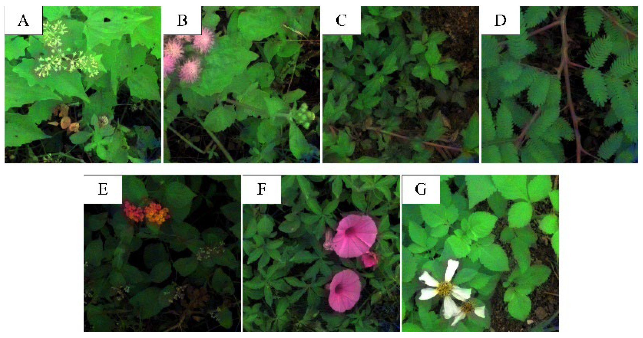
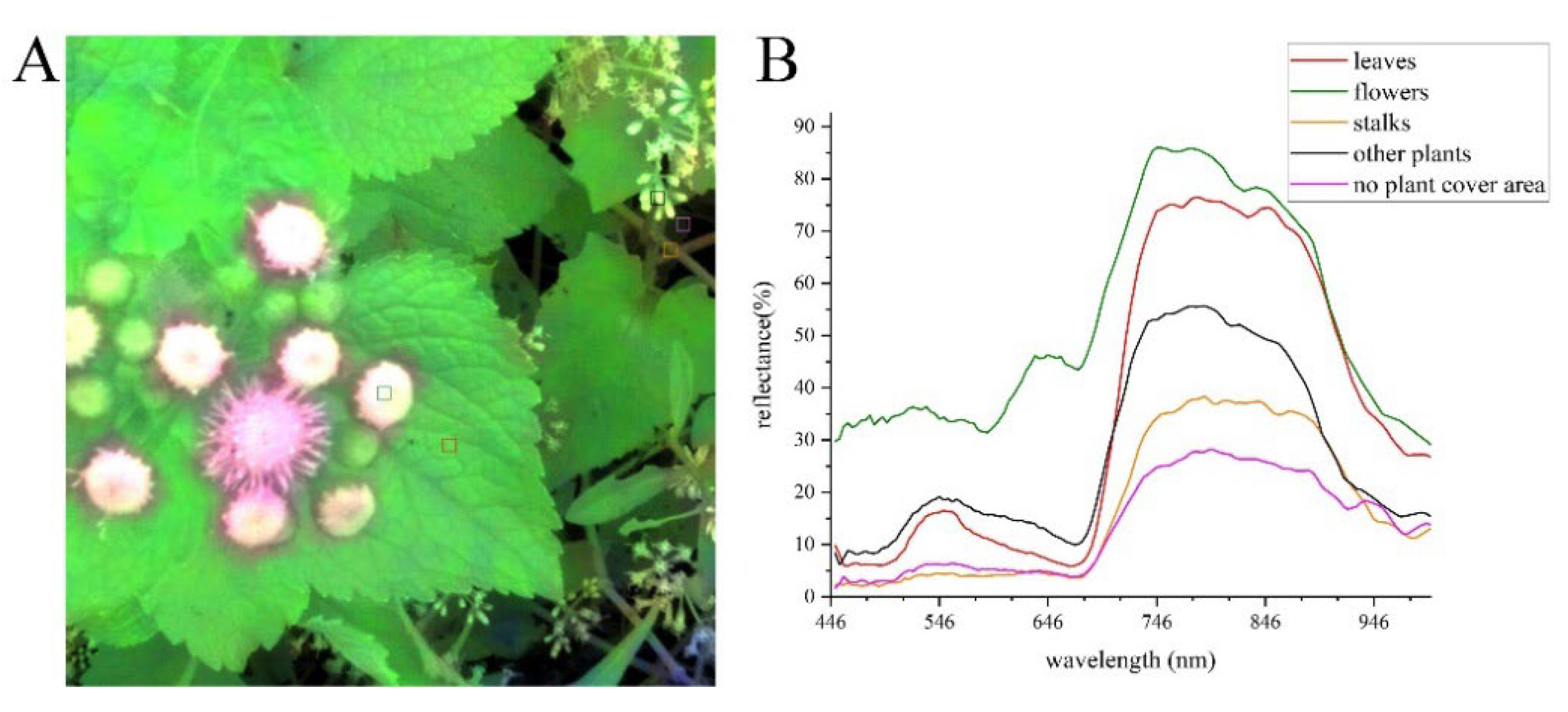
Then, the spectrometer’s lens was aimed directly at the surface of the invasive plant and manually focused to the middle of the leaves. Eighty images of vegetation were collected using the hyperspectral camera and were used in this study. Partial samples of seven invasive plants are shown in
Figure 1. The images contain leaves, flowers, stalks, other plants and the no-plant cover area. Among them, flowers, stalks and the no-plant cover area belong to background. The leaves and background feature points were extracted manually from the original images using Cubeware software (approximately 43 per image, 38 of which are leaves feature points), as shown in
Figure 2A; the spectral curves are shown in
Figure 2B and saved in ASCII format. In this work, 3359 raw spectral data samples (
M. micrantha: 428, background: 409,
S. calendulacea: 428,
A. conyzoides: 425,
M. pudica: 419,
L. camara: 408,
L. cairica: 418,
B. pilosa: 424) were collected, including a random partition a training set (2400 samples, each category has 300 samples) and testing set (959 samples).
2.2. Preprocessing Methods
Hyperspectral data have a large amount of interference redundancy information, which seriously affects the accuracy of the identification. Studies have shown that the interference of noise, astigmatism and baseline drift caused by human factors and background can be reduced by preprocessing [
30]. At present, preprocessing methods are relatively mature and can be divided into derivative algorithms, smoothing algorithms, and light scattering correction algorithms. FD, SG smoothing and SNV were used in this paper.
2.2.1. First Derivative
First derivatives (FD) can reduce hyperspectral mutual interference and reduce noise in the analysis of hyperspectral data [
31], and they are often used for baseline correction and background elimination in hyperspectral analysis [
32]. The formula for spectral reflectance for the FD at wavelength point
k can be solved as follows:
In the above formula, k is the window width, .
2.2.2. Savitzky–Golay Smoothing
The smoothing methods include moving window smoothing and Savitzky–Golay (SG) convolution smoothing [
33]. Compared with the moving window smoothing method, SG convolution smoothing can achieve a better denoising effect because moving window smoothing is limited by the number of windows. If the number of windows is too large or too small, the denoising effect will be affected. The two smoothing methods are similar, but the difference is that SG convolution smoothing focuses on the calculation of the central value, while moving window smoothing focuses on the number of windows. That is, SG smoothing is an algorithm based on polynomial smoothing, which smooths the spectral curve through moving windows combined with least squares fitting. Its calculation formula is as follows:
where
is the smoothing coefficient,
is the smoothed value of
k points,
is the unsmoothed value of
k,
i is the number of smoothed data points from this point to the left,
m refers to the number of smoothed data points from this point to the right, and
N is the normalization factor.
2.2.3. Standard Normal Variable Transformation
The standard normal variate (SNV) transformation is mainly used to eliminate the influence of solid particle size, surface scattering and optical path changes on the reflected spectrum [
34]. SNV is the same as the standardized algorithm, except that the standardized algorithm addresses a set of spectra (based on the column of the spectral array), while SNV addresses a spectrum (based on the row of the spectrum) [
35].
on the type of
,
m is the number of wavelength points.
2.3. Dimension Reduction
The raw and preprocessing spectral data are 138-dimensional, and a high number of dimensions may lead to low efficiency of hyperspectral modeling and poor model performance. Therefore, it is necessary to reduce the dimensionality of hyperspectral data and retain most of the dataset information. Many studies have shown that the dimensionality reduction processing of hyperspectral data can not only shorten the time but can also improve the recognition efficiency to some extent [
36]. In this paper, PCA and ACO were used to reduce the dimensionality of hyperspectral data of invasive plants.
2.3.1. Principal Component Analysis
PCA is a dimensionality reduction method that transforms multidimensional data features into a few comprehensive features and uses variable information represented by a few variable features [
37,
38]. The PCA dimension reduction transformation process is as follows: suppose that the n-dimensional preprocessing result variable (
) to perform the linear transformation of Formula (5) on variable
(
= 1, 2, 3,
) to obtain the comprehensive variable (
) is,
Equation (5) linear transformation satisfies the following conditions:
(1) are linearly independent;
(2) + = 1, ( = 1, 2, 3, );
(3) the composite variables are arranged according to their variances.
The process of PCA is based on the contribution rate of a single principal component and the cumulative contribution rate. When the cumulative contribution rate of the first m principal components reaches 85%, the first
m principal components can represent most of the information of the n-dimensional data to achieve dimensionality reduction. The calculation formulas of the principal component contribution rate and cumulative contribution rate are as follows:
In Formulas (6) and (7), is the principal component contrast.
2.3.2. Ant Colony Optimization
ACO is a probabilistic dimension reduction method for spectral feature selection of hyperspectral data [
38]. Based on ACO, the main idea is to feature the selection problem of modeling for solving the minimum cost path search graph, thus creating a node of the search space and design procedures to find the manners of solution. ACO states the path that the ant chooses of the choice probability of the feature subset, based on the pheromone and heuristic information to compute the ant’s choice. In this paper, the Fisher criterion is used to calculate heuristic information, and the ant’s transition from one node to another node is determined by probability. Assume that the transfer probability
of ant
k from node
i to node
j at time
t is calculated by the following formula:
When the ant completes a cycle, the pheromone on each path is calculated as follows:
refers to the pheromone concentration on the path from node
i to node
j at time
t, and
is the heuristic function, which refers to the expectation of ant
k choosing to remove node
j from node
i. The calculation formula is as follows:
where
is the distance from node
i to node
j. The value of
= 1, 2, …, n − 1,
is the total number of nodes,
represents the nodes that ant
k can select next,
is the weight parameter, which plays a role in the importance of pheromones and heuristics,
is the pheromone evaporation coefficient, and
is the pheromone concentration increment on the path from node
i to node
j.
2.4. Identification Models
The typical algorithms based on hyperspectral image data classification include the neighborhood algorithm, SVM, RF, and neural network. Domestic and foreign researchers have accomplished many achievements on invasive plants based on hyperspectral data, most of which are based on the spatial distribution [
39], area extraction [
40], and species identification of invasive plants [
41]. According to the characteristics of the samples, SVM and RF were selected to identify seven invasive plants.
SVM is a classical machine learning algorithm based on traditional theory; the core content of this is to transform the object of our study into a high-dimensional feature space by nonlinear transformation and to construct a linear decision function in the high-dimensional space to realize the nonlinear decision function of the original space [
42]. In this paper, the kernel function selected by SVM classifier is the radical basis function (RBF). For each SVM model, a grid search combined with a 5-fold cross validation method was used to optimize parameters. The search interval of the penalty coefficient and kernel parameter was set as 2
−5~2
5, the step size was 0.1.
RF is a combination of classification trees that implements randomization [
43]. In the 1980s, Breiman et al. invented the classification tree algorithm [
44]. It is calculated by repeating dichotomous data. In the same year, Breiman merged classification trees into random forests. RF generate multiple classification trees by randomizing the data and variables, and then obtaining statistical results. The main parameters of RF are the number of trees and the number of nodes. In this paper, the number of trees was set to 1000, and the number of nodes was set to 10 for all of the RF models.
2.5. Performance Evaluation
The performance of all of the combined models was evaluated based on four statistical parameters, namely, accuracy (A), average accuracy (AA), average precision (AP) and test time, which were often used to evaluate the performance of the classification models and calculated from Equations (11) and (12) [
45].
where
TP is the true positive sample,
TN is the true negative sample,
FN is the false negative sample,
FP is the false positive sample,
N is the total sample number,
i is the number of categories.
All of the aforementioned steps were coded and developed in the environment of MATLAB R2020a (The Math Works Inc., Natick, MA, USA). The GPU of the PC is a NVIDIA GTX 3060.
3. Results
3.1. Preprocessing
Raw and preprocessing spectral data of seven invasive plants and background are shown in
Figure 3A–D. In
Figure 3A,
M. micrantha has the highest reflectivity in the wavelength range of approximately 700 to 900 nm, followed by
B. pilosa,
M. pudica,
L. cairica,
A. conyzoides,
S. calendulacea and
L. camara. In the range of approximately 450 to 680 nm, the background reflectance is relatively scattered, while in the range of approximately 700 nm to 998 nm, the background overlaps with the spectral reflectance of seven invasive species, and the overlap region between species was large. Therefore, it is challenging to classify seven invasive species simultaneously. To facilitate the identification of raw spectral data, three processing methods were used to reduce data noise and highlight the distribution patterns of reflectivity with wavelength. The original spectral data processed by SG smoothing are shown in
Figure 3C. Compared with
Figure 3A, the curve of
Figure 3C is relatively smooth, and small fluctuations in reflectance over the whole wavelength range are eliminated. The other two processing methods, FD and SNV, remove other noise from the original spectral data.
Figure 3B presents the FD processing of direct difference analysis of the raw spectral data, that is, noise reduction is performed at both ends of the spectral band. Compared with
Figure 3B, the raw spectral data are obviously interfered with by artificial and systematic noises, and the intraclass difference of spectral data after FD processing is less than that of the original spectral data.
Figure 3D displays the preprocessing data of SNV, and the intraclass difference in spectral data is reduced.
In summary, all three preprocessing methods can eliminate part of the spectral noise. SG smoothing reduced the small range of spectral fluctuations, FD and SNV reduced the intra-class differences in species, but none of the processing methods significantly reduced the inter-class differences in species and background. Therefore, it is necessary to determine the inter-class differences of the seven species through subsequent treatments. To determine a more appropriate pretreatment method, the next step is to analyze the impact of each processing method combined with dimension reduction.
3.2. Dimension Reduction by PCA
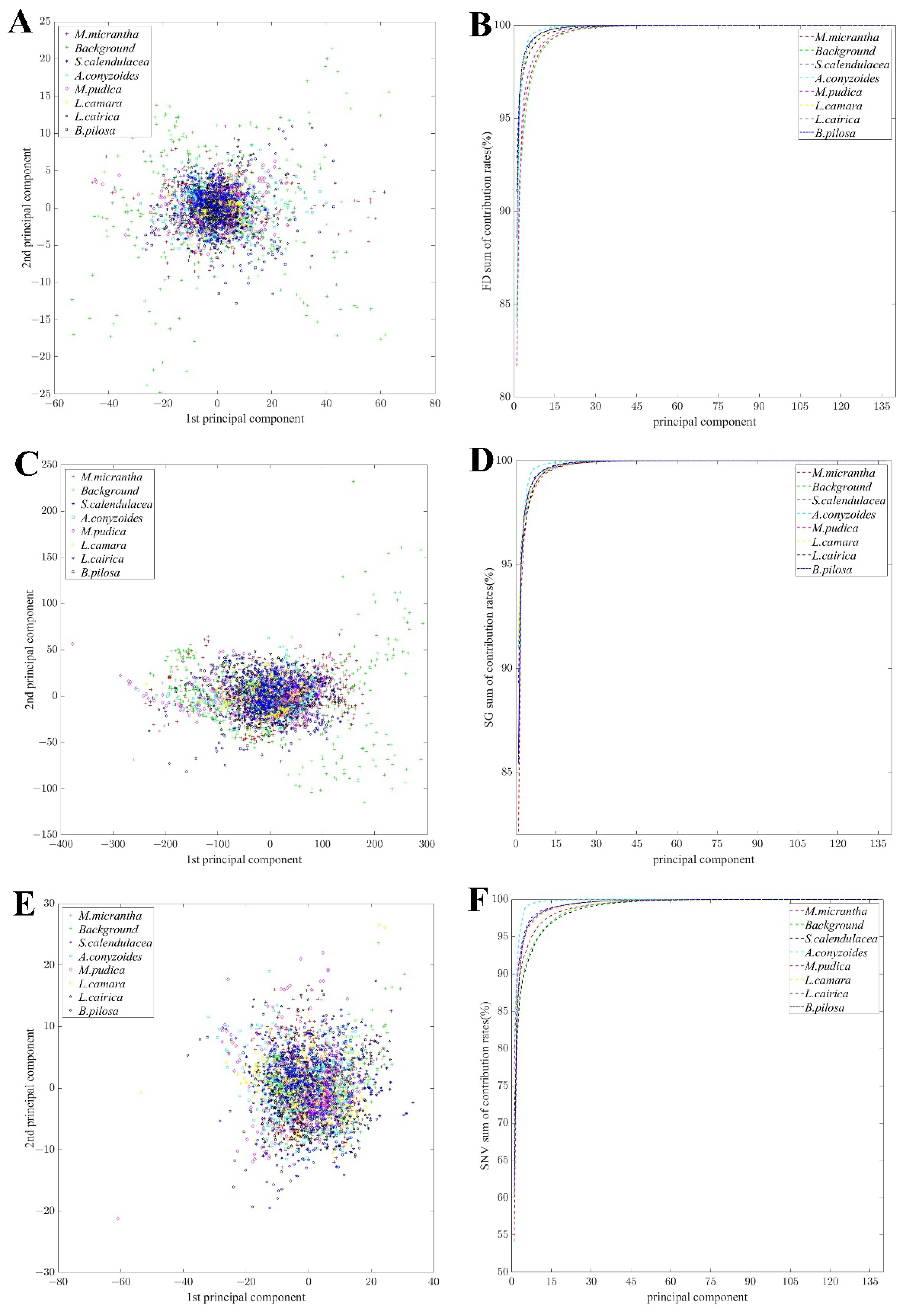
Based on the preprocessing results, dimension reduction analysis was conducted by PCA, as shown in
Figure 4A,C,E, which are the point states drawn in horizontal (first principal component scores) and vertical (second principal component scores) coordinates. In this way, we can preliminarily judge the convergence degree of FD, SG smoothing and SNV. According to
Figure 4A,C,E, it is obvious that FD-PCA has a better sample clustering effect, but
S. calendulacea,
L. camara and
B. pilosa overlap clearly. In
Figure 4C, the seven invasive plants are relatively scattered; that is, after SG-PCA treatment, the sample points of invasive plants have almost no similar convergence. In terms of clustering performance, FD ranked first, SNV ranked second, and SG ranked third. The worst clustering performance of SG smoothing preprocessing is predictable because SG smoothing reduces noise but does not change details and overall trends. Therefore, more components need to be considered later.
The cumulative contribution rate of the first 138 principal components were calculated as shown in
Figure 4B,D,F. It is clear that at around the first 22 principal components, all curves tended to be smooth and the cumulative principal component contribution rate approaches 100%. Therefore, the principal component characteristics of the first 22 dimensions can fully represent the spectral information of 138 dimensions. In other words, after PCA, the 138-dimensional spectrum is reduced to 22 dimensions.
3.3. Dimension Reduction by ACO
Based on the preprocessing results, feature selection was carried out by ACO, and the feature bands are shown in
Table 1.
The number of feature bands selected based on FD was 28, SNV was 25 and SG was 20.
Table 1 shows that the feature bands selected based on the three preprocessing methods are concentrated in the range of 450–700 nm. That is, the feature wavelengths are concentrated in the visible range.
Wavelengths of 450, 454, 458, 462, 466, 470, 474, 478, 482, 486, 494, 510, 518 and 526 nm were common to all three preprocessing methods, indicating that these wavelengths were important features in distinguishing the seven species. Based on ACO, the extracted feature wavelengths were relatively continuous between 450–700 nm and relatively scattered between 700–998 nm. Furthermore, the selection of feature wavelengths is related to the quality of the preprocessing. After all, the number of feature wavelengths extracted based on SG is the lowest and the number based on FD is the highest.
3.4. Identification Performance Evaluation of Different Combination Models
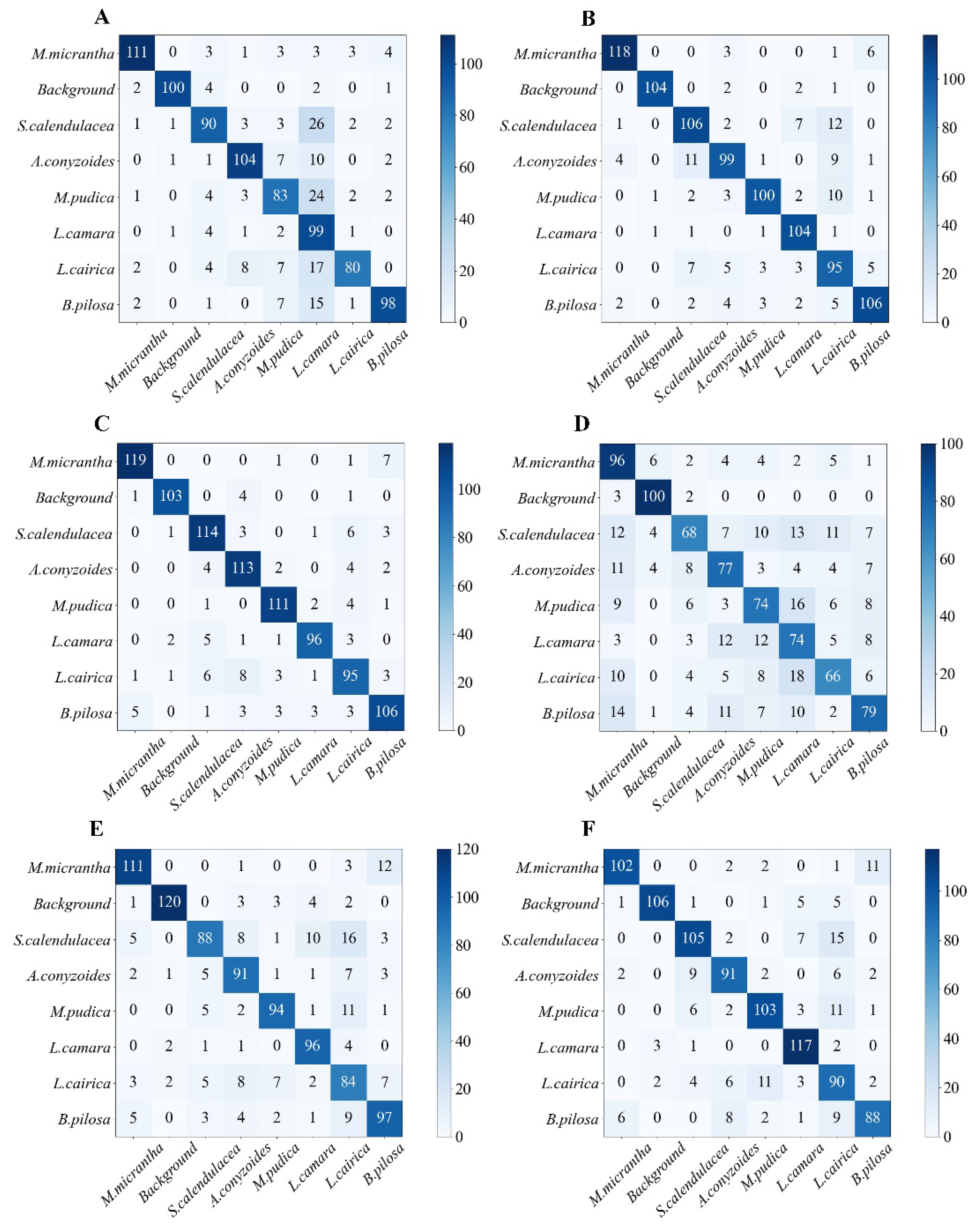
Among the 3359 samples, 2400 samples were used for model training and 959 samples were used for model testing. To explore the single species recognition rates and total recognition rates for each combined model, confusion matrices, single species recognition accuracy tables and total accuracy tables are presented, as shown in
Figure 5,
Table 2 and
Table 3 (
Figure 5 and
Table 2 only present the models with the highest accuracy under the same conditions).
SG-SVM showed outstanding advantages in the identification process among nearly all species. The SG-SVM identified 92.97%, 89.06%, 90.40%, 93.28%, 80.51% and 85.49% accuracy for M. micrantha, S. calendulacea, A. conyzoides, M. pudica, L. cairica and B. Pilosa, respectively, which are far better than those of SNV-PCA-SVM (86.72%, 70.31%, 83.20%, 69.75%, 67.80%, 79.03%), SNV-PCA-RF (80.00%, 51.51%, 65.25%, 60.66%, 56.41%, 61.72%). Meanwhile, the total accuracy (A), the average accuracy (AA), the average precision (AP) of SG-SVM are also excellent, reaching 89.36%, 89.39% and 89.54%, respectively. SG-ACO-SVM (86.76%, 86.99%, 87.22%) cannot be ignored. Compared to SG-SVM, the test time is also shorter, although A, AA and AP are all reduced. When the A of the model was reduced by about 3%, the cost time was nearly 5 times shorter. Moreover, for L. camara recognition, SG-ACO-SVM (96.30%) is superior to SG-SVM (88.89%). SG-SVM and SG-ACO-SVM show advantages in recognition accuracy and time cost, respectively. In practice, when the total accuracy is relatively important, the SG-SVM model is selected, and when the test time cost is relatively important, the SG-ACO-SVM model is used.
4. Discussion
Currently, manual monitoring is still the mainstay of invasive plant monitoring. However, this makes the monitoring of invasive species both laborious and time-consuming. Given these facts, unmanned aerial vehicle (UAV) with hyperspectral cameras can offer significant opportunities for invasive plant monitoring. Hyperspectral remote sensing, which combines the advantages of imaging and spectroscopy, has been successfully applied to invasive plant monitoring. Previous studies using hyperspectral imaging to monitor the spectral information of invasive plants at different time periods have been very effective. The results obtained in this study show that the spectral distribution of different invasive plants during the same period is different, but the differences are not significant. In general, the lower reflectance of invasive plants occurs in the visible part of the spectrum (400–700 nm), and the absorption of photosynthetic pigments in the region associated with it is largely concentrated in the blue (450-chlorophyll b) and red (650-chlorophyll a) regions.
The highest total accuracy of the combined model in this paper was only 89.39%. On the one hand, only traditional machine learning models are used, on the other hand, SVM and RF is mostly suitable for binary classification [
46,
47]. After all, SVM and RF can often achieve high accuracy in the application of binary classification [
48]. Although the LIBSVM toolbox is capable of solving multiclassification problems [
49], the total classification accuracy of samples is not high because the difference of spectral features between various samples is not big, or the difference of features between samples is further reduced after normalization. Dimensionality reduction reduces the training and testing time of the model, but inevitably leads to the loss of some important information, which is the main reason why the accuracy of dimensionality reduction models is lower than that of non-dimensionality reduction models. Of course, the small amount of data is also an important reason. Therefore, it is necessary to expand the datasets or try to use a new type of model to improve the accuracy and efficiency.
Recent studies have used hyperspectral imaging combined with deep learning methods to monitor invasive plants [
50,
51]. Meanwhile, deep learning is very popular in species classification [
52,
53], but it does not mean that the recognition effect of deep learning is superior to that of other algorithms. For example, in the recognition of grapevine species, the recognition effect of a SVM is not inferior to that of a convolutional neural network [
54]. However, it cannot be denied that deep learning is a current trend in image recognition. To further improve the accuracy of recognition, it is necessary to adopt a deep learning algorithm.
By studying the leaf spectra of the seven invasive plants, 18 combination models were able to distinguish seven invasive plants within a short time interval. By analyzing different combination models, it is found that the total accuracy of SG-SVM is the highest, followed by SG-ACO-SVM. It is worth noting that the spectrum of SG-ACO-SVM was only 20-dimensional, while the spectrum of SG-SVM was 138-dimensional. Although the total accuracy of the SG-ACO-SVM is slightly less, the testing time has been significantly shortened. Of course, the reduction in dimensionality does not necessarily indicate that the models will take less time to test. After all, the SG-PCA-RF and SNV-PCA-RF models are more time consuming than their non-dimensional reduction counterparts. However, the training time for the reduced dimension models is clearly lower than that for the non-dimensional reduction models, and this is true for all of the combined models. While the total accuracy is reduced, a satisfactory recognition accuracy is obtained in a shorter period of time. This is the purpose of using dimensionality reduction and the reason for comparing the 18 combined models.
In this paper, seven invasive plants were identified using 18 models, though promising, in-depth research is necessary before the technique can be applied to the field for accurate monitoring. One aspect that should be considered in future research is the spectral monitoring of invasive plants over their entire period. On the other hand is the consideration of the average spectra of more organs of the invasive plant, such as the flowers, stems, leaves, etc. of the plant. To achieve this, operational challenges have to be overcome. Such as the selection and collection of optimal conditions for hyperspectral images of the plant under test, the determination of the spectral distributions and correlated color temperatures of solar radiations, the calibration of black and white under different atmospheric conditions, the possibility of mounting a hyperspectral sensor on an unmanned aircraft, the calibration of the sensor, the collection, storage and analysis.
The main work of this research was to complete the identification of seven invasive species in four small fields. The image samples used were hyperspectral images taken with a handheld spectrometer. In practical applications, it is often necessary to identify a large range of invasive plants, which requires the installation of a hyperspectral imager on a UAV for image acquisition. Our study provides a reliable reference for hyperspectral image data processing and the classification of a variety of invasive plants.
5. Conclusions
Hyperspectral data of invasive plants in the wild were used as sample data in this work, and three groups of different results were obtained by different preprocessing methods (FD, SG, and SNV). Based on the three preprocessing results, nine groups of data were obtained by combining dimensionality reduction (PCA, ACO) and no dimensionality. The nine groups of data were combined with classification methods (SVM and RF) to establish different classification models to obtain the best recognition method for invasive plants.
The results show that the SG preprocessing method has a better preprocessing effect on hyperspectral data, and most values of the models obtained under this condition are optimal. Based on the preprocessing results, by comparing the results of dimensionality reduction and no dimensionality reduction, the method of dimension reduction may not improve the accuracy of recognition, but it can improve time efficiency. Compared with the RF classifier, the SVM classifier has a better recognition effect on invasive plants. In the dimension reduction method based on PCA and ACO, SVM model recognition based on the ACO dimension reduction method is better. Among the 18 models, the 2 best models are SG-ACO-SVM (AA, 86.99%, AP, 87.22%, TT, 0.0567) and SG-SVM (AA, 89.39%, AP, 89.54%, test time, 0.2639).
Author Contributions
X.Q. and Y.H.: methodology, software, validation, writing. X.L.: methodology, software, validation, writing-original draft, writing-review. F.W.: software. Z.S. and L.Y.: project administration. X.P. and S.L.: project administration. W.Q.: project administration, Writing-original draft, Writing-review and editing. All authors contributed to the article and approved the submitted version. All authors have read and agreed to the published version of the manuscript.
Funding
The work in this paper was supported by the National Natural Science Foundation of China (32272633, 61871475), the Key Research and Development Program of Nanning (20192065), and the Guangdong Science and Technology Planning Project (2017A020216022).
Data Availability Statement
Not applicable.
Acknowledgments
The authors thank the native English-speaking experts for polishing our paper.
Conflicts of Interest
The authors declare no conflict of interest.
References
- Pan, X.B.; Zhang, J.Q.; Xu, H.; Zhang, X.L.; Zhang, W.; Song, H.H.; Zhu, S.F. Spatial similarity in the distribution of invasive alien plants and animals in China. Nat. Hazards 2015, 77, 1751–1764. [Google Scholar] [CrossRef]
- Liu, Y.J.; Oduor, A.M.O.; Zhang, Z.; Manea, A.; Tooth, I.M.; Leishman, M.R.; Xu, X.L.; Van Kleunen, M. Do invasive alien plants benefit more from global environmental change than native plants? Glob. Chang. Biol. 2017, 23, 3363–3370. [Google Scholar] [CrossRef] [PubMed] [Green Version]
- Miller, K.M.; McGill, B.J.; Weed, A.S.; Seirup, C.E.; Comiskey, J.A.; Matthews, E.R.; Perles, S.; Schmit, J.P. Long-term trends indicate that invasive plants are pervasive and increasing in eastern national parks. Ecol. Appl. 2021, 31, e02239. [Google Scholar] [CrossRef] [PubMed]
- Nguyen, N.A.; Eskelson, B.N.I.; Meitner, M.J.; Murray, T. People’s Knowledge and Risk Perceptions of Invasive Plants in Metro Vancouver, British Columbia, Canada. Environ. Manag. 2020, 66, 985–996. [Google Scholar] [CrossRef] [PubMed]
- Qian, W.Q.; Huang, Y.Q.; Liu, Q.; Fan, W.; Sun, Z.Y.; Dong, H.; Wan, F.H.; Qiao, X. UAV and a deep convolutional neural network for monitoring invasive alien plants in the wild. Comput. Electron. Agric. 2020, 174, 105519. [Google Scholar] [CrossRef]
- Carlier, J.; Davis, E.; Ruas, S.; Byrne, D.; Caffrey, J.M.; Coughlan, N.E.; Dick, J.T.A.; Lucy, F.E. Using open-source software and digital imagery to efficiently and objectively quantify cover density of an invasive alien plant species. J. Environ. Manag. 2020, 266, 110519. [Google Scholar] [CrossRef]
- Cohen, J.G.; Lewis, M.J. Development of an Automated Monitoring Platform for Invasive Plants in a Rare Great Lakes Ecosystem Using Uncrewed Aerial Systems and Convolutional Neural Networks. In Proceedings of the International Conference on Unmanned Aircraft Systems (ICUAS), Athens, Greece, 1–4 September 2020; pp. 1553–1564. [Google Scholar]
- Ma, Y.; Liu, X.; Liu, M.; Shi, L.; Zhang, Z.; Zhao, N. Feature analysis and model monitoring of different florescences of Mikania micrantha based on hyper-spectrum imaging. J. Yunnan Univ.-Nat. Sci. Ed. 2021, 43, 290–298. [Google Scholar] [CrossRef]
- Qiu, Y.; Lu, J. Dynamic simulation of Spartina alterniflora based on CA-Markov model-a case study of Xiangshan bay of Ningbo City, China. Aquat. Invasions 2018, 13, 299–309. [Google Scholar] [CrossRef]
- Liu, M.; Mao, D.; Wang, Z.; Li, L.; Man, W.; Jia, M.; Ren, C.; Zhang, Y. Rapid Invasion of Spartina alterniflora in the Coastal Zone of Mainland China: New Observations from Landsat OLI Images. Remote Sens. 2018, 10, 1933. [Google Scholar] [CrossRef] [Green Version]
- Ren, G.; Zhou, L.; Liang, J.; Lu, F.; Wang, A.; Wang, J.; Li, X.; Ma, Y. Monitoring the Invasion of Spartina Alterniflora Using Hyperspectral Remote Sensing Image of GF-5. Adv. Mar. Sci. 2021, 39, 312–326. [Google Scholar]
- Barbosa, J.M.; Asner, G.P.; Martin, R.E.; Baldeck, C.A.; Hughes, F.; Johnson, T. Determining Subcanopy Psidium cattleianum Invasion in Hawaiian Forests Using Imaging Spectroscopy. Remote Sens. 2016, 8, 33. [Google Scholar] [CrossRef]
- Khare, S.; Latifi, H.; Ghosh, S.K. Multi-scale assessment of invasive plant species diversity using Pleiades 1A, RapidEye and Landsat-8 data. Geocarto Int. 2018, 33, 681–698. [Google Scholar] [CrossRef]
- Gosselin, H.; Sagan, V.; Maimaitiyiming, M.; Fishman, J.; Belina, K.; Podleski, A.; Maimaitijiang, M.; Bashir, A.; Balakrishna, J.; Dixon, A. Using Visual Ozone Damage Scores and Spectroscopy to Quantify Soybean Responses to Background Ozone. Remote Sens. 2020, 12, 93. [Google Scholar] [CrossRef] [Green Version]
- Tarantino, C.; Casella, F.; Adamo, M.; Lucas, R.; Beierkuhnlein, C.; Blonda, P. Ailanthus altissima mapping from multi-temporal very high resolution satellite images. Isprs J. Photogramm. Remote Sens. 2019, 147, 90–103. [Google Scholar] [CrossRef]
- Xu, Y.; Zhang, C.; Jiang, R.; Wang, Z.; Zhu, M.; Shen, G. UAV-based hyperspectral images and monitoring of canopy tree diversity. Biodivers. Sci. 2021, 29, 647–660. [Google Scholar] [CrossRef]
- Zheng, D.; Shen, G.; Wang, B.; Dai, G.; Lin, F.; Hu, J.; Ye, J.; Fang, S.; Hao, Z.; Wang, X.; et al. Classification of dominant species in coniferous and broad-leaved mixed forest on Changbai Mountain based on UAV-based hyperspectral image and deep learning algorithm. Chin. J. Ecol. 2022, 41, 1024–1032. [Google Scholar]
- Sabat-Tomala, A.; Raczko, E.; Zagajewski, B. Comparison of Support Vector Machine and Random Forest Algorithms for Invasive and Expansive Species Classification Using Airborne Hyperspectral Data. Remote Sens. 2020, 12, 516. [Google Scholar] [CrossRef] [Green Version]
- Liu, Y.; Chang, M.; Xu, J. High-Resolution Remote Sensing Image Information Extraction and Target Recognition Based on Multiple Information Fusion. IEEE Access 2020, 8, 121486–121500. [Google Scholar] [CrossRef]
- Yan, R.; Peng, J.; Ma, D. Dimensionality reduction based on parallel factor analysis model and independent component analysis method. J. Appl. Remote Sens. 2019, 13, 014532. [Google Scholar] [CrossRef]
- Sun, H.; Zhang, L.; Rao, Z.H.; Ji, H.Y. Determination of moisture content in barley seeds based on hyperspectral imaging technology. Spectrosc. Lett. 2020, 53, 751–762. [Google Scholar] [CrossRef]
- Pang, L.; Xiao, J.; Ma, J.J.; Yan, L. Hyperspectral imaging technology to detect the vigor of thermal-damaged Quercus variabilis seeds. J. For. Res. 2021, 32, 461–469. [Google Scholar] [CrossRef]
- Shen, L.; Gao, M.; Yan, J.; Li, Z.L.; Duan, S.B.J.R.S. Hyperspectral Estimation of Soil Organic Matter Content using Different Spectral Preprocessing Techniques and PLSR Method. Remote Sens. 2020, 12, 1206. [Google Scholar] [CrossRef]
- Xu, H.; Zhang, H.; He, W.; Zhang, L. Superpixel-based spatial-spectral dimension reduction for hyperspectral imagery classification. Neurocomputing 2019, 360, 138–150. [Google Scholar] [CrossRef]
- Garcia-Salgado, B.P.; Ponomaryov, V.I.; Sadovnychiy, S.; Reyes-Reyes, R. Efficient dimension reduction of hyperspectral images for big data remote sensing applications. J. Appl. Remote Sens. 2020, 14, 032611. [Google Scholar] [CrossRef]
- Yang, Q.L.; Wan, X.X.; Xiao, G.S. Multispectral Dimension Reduction Algorithm Based on Partial Least Squares. Laser Optoelectron. Prog. 2020, 57, 013003. [Google Scholar] [CrossRef]
- Papp, L.; van Leeuwen, B.; Szilassi, P.; Tobak, Z.; Szatmari, J.; Arvai, M.; Meszaros, J.; Pasztor, L. Monitoring Invasive Plant Species Using Hyperspectral Remote Sensing Data. Land 2021, 10, 29. [Google Scholar] [CrossRef]
- Bellia, L.; Blaszczak, U.; Fragliasso, F.; Gryko, L. Matching CIE illuminants to measured spectral power distributions: A method to evaluate non-visual potential of daylight in two European cities. Sol. Energy 2020, 208, 830–858. [Google Scholar] [CrossRef]
- Huang, Y.; Li, J.; Yang, R.; Wang, F.; Li, Y.; Zhang, S.; Wan, F.; Qiao, X.; Qian, W. Hyperspectral Imaging for Identification of an Invasive Plant Mikania micrantha Kunth. Front. Plant Sci. 2021, 12, 626516. [Google Scholar] [CrossRef]
- Ge, X.-Y.; Ding, J.-L.; Wang, J.-Z.; Sun, H.-L.; Zhu, Z.-Q. A New Method for Predicting Soil Moisture Based on UAV Hyperspectral Image. Spectrosc. Spectr. Anal. 2020, 40, 602–609. [Google Scholar] [CrossRef]
- Saberioon, M.; Cisar, P.; Labbe, L.; Soucek, P.; Pelissier, P. Spectral imaging application to discriminate different diets of live rainbow trout (Oncorhynchus mykiss). Comput. Electron. Agric. 2019, 165, 104949. [Google Scholar] [CrossRef]
- Golhani, K.; Balasundram, S.K.; Vadamalai, G.; Pradhan, B. Estimating chlorophyll content at leaf scale in viroid-inoculated oil palm seedlings (Elaeis guineensis Jacq.) using reflectance spectra (400 nm–1050 nm). Int. J. Remote Sens. 2019, 40, 7647–7662. [Google Scholar] [CrossRef]
- Feng, J.; Liu, Y.H.; Shi, X.W.; Wang, Q.Q. Potential of hyperspectral imaging for rapid identification of true and false honeysuckle tea leaves. J. Food Meas. Charact. 2018, 12, 2184–2192. [Google Scholar] [CrossRef]
- Asaari, M.S.M.; Mishra, P.; Mertens, S.; Dhondt, S.; Inze, D.; Wuyts, N.; Scheunders, P. Close-range hyperspectral image analysis for the early detection of stress responses in individual plants in a high-throughput phenotyping platform. Isprs J. Photogramm. Remote Sens. 2018, 138, 121–138. [Google Scholar] [CrossRef]
- Liu, J.B.; Han, J.C.; Chen, X.; Shi, L.; Zhang, L. Nondestructive detection of rape leaf chlorophyll level based on Vis-NIR spectroscopy. Spectrochim. Acta Part A-Mol. Biomol. Spectrosc. 2019, 222, 117202. [Google Scholar] [CrossRef]
- Hamim, M.; El Moudden, I.; Pant, M.D.; Moutachaouik, H.; Hain, M. A Hybrid Gene Selection Strategy Based on Fisher and Ant Colony Optimization Algorithm for Breast Cancer Classification. Int. J. Online Biomed. Eng. 2021, 17, 148–163. [Google Scholar] [CrossRef]
- Weng, S.; Tang, P.; Yuan, H.; Guo, B.; Yu, S.; Huang, L.; Xu, C. Hyperspectral imaging for accurate determination of rice variety using a deep learning network with multi-feature fusion. Spectrochim. Acta Part A-Mol. Biomol. Spectrosc. 2020, 234, 118237. [Google Scholar] [CrossRef]
- Bonah, E.; Huang, X.; Yi, R.; Aheto, J.H.; Yu, S. Vis-NIR hyperspectral imaging for the classification of bacterial foodborne pathogens based on pixel-wise analysis and a novel CARS-PSO-SVM model. Infrared Phys. Technol. 2020, 105, 103220. [Google Scholar] [CrossRef]
- Masemola, C.; Cho, M.A.; Ramoelo, A. Assessing the Effect of Seasonality on Leaf and Canopy Spectra for the Discrimination of an Alien Tree Species, Acacia Mearnsii, From Co-Occurring Native Species Using Parametric and Nonparametric Classifiers. IEEE Trans. Geosci. Remote Sens. 2019, 57, 5853–5867. [Google Scholar] [CrossRef]
- Kopec, D.; Zakrzewska, A.; Halladin-Dabrowska, A.; Wylazlowska, J.; Kania, A.; Niedzielko, J. Using Airborne Hyperspectral Imaging Spectroscopy to Accurately Monitor Invasive and Expansive Herb Plants: Limitations and Requirements of the Method. Sensors 2019, 19, 2871. [Google Scholar] [CrossRef] [Green Version]
- Kganyago, M.; Odindi, J.; Adjorlolo, C.; Mhangara, P. Evaluating the capability of Landsat 8 OLI and SPOT 6 for discriminating invasive alien species in the African Savanna landscape. Int. J. Appl. Earth Obs. Geoinf. 2018, 67, 10–19. [Google Scholar] [CrossRef]
- Wang, C.X.; Wang, S.L.; He, X.G.; Dong, H. The Identification of Beef Varieties by Fusing Image Information Based on Hypersepctral Image Technology. Spectrosc. Spectr. Anal. 2020, 40, 911–916. [Google Scholar] [CrossRef]
- Huang, H.; Liu, J.; Liu, S.; Wu, T.; Jin, P. A method for classifying tube structures based on shape descriptors and a random forest classifier. Measurement 2020, 158, 107705. [Google Scholar] [CrossRef]
- Breiman, L. Random forests. Mach. Learn. 2001, 45, 5–32. [Google Scholar] [CrossRef] [Green Version]
- Dash, J.P.; Watt, M.S.; Paul, T.S.H.; Morgenroth, J.; Pearse, G.D. Early Detection of Invasive Exotic Trees Using UAV and Manned Aircraft Multispectral and LiDAR Data. Remote Sens. 2019, 11, 1812. [Google Scholar] [CrossRef] [Green Version]
- Hsu, C.W.; Lin, C.J. A comparison of methods for multiclass support vector machines. IEEE Trans. Neural Netw. 2002, 13, 415–425. [Google Scholar] [CrossRef] [Green Version]
- Xia, S.; Chen, B.; Wang, G.; Zheng, Y.; Gao, X.; Giem, E.; Chen, Z. mCRF and mRD: Two Classification Methods Based on a Novel Multiclass Label Noise Filtering Learning Framework. IEEE Trans. Neural Netw. Learn. Syst. 2022, 33, 2916–2930. [Google Scholar] [CrossRef]
- Li, L.; Li, L.; Wu, Y.; Ye, M. Experimental Comparisons of Multi-class Classifiers. Inform.-J. Comput. Inform. 2015, 39, 71–85. [Google Scholar]
- Liu, M. English speech emotion recognition method based on speech recognition. Int. J. Speech Technol. 2022, 25, 391–398. [Google Scholar] [CrossRef]
- Theron, J.; Pryke, J.S.; Latte, N.; Samways, M.J. Mapping an alien invasive shrub within conservation corridors using super-resolution satellite imagery. J. Environ. Manag. 2022, 321, 116023. [Google Scholar] [CrossRef]
- Zhao, H.; Zhong, Y.; Wang, X.; Hu, X.; Luo, C.; Boitt, M.; Piiroinen, R.; Zhang, L.; Heiskanen, J.; Pellikka, P. Mapping the distribution of invasive tree species using deep one-class classification in the tropical montane landscape of Kenya. Isprs J. Photogramm. Remote Sens. 2022, 187, 328–344. [Google Scholar] [CrossRef]
- Gonzalez-Perez, A.; Abd-Elrahman, A.; Wilkinson, B.; Johnson, D.J.; Carthy, R.R. Deep and Machine Learning Image Classification of Coastal Wetlands Using Unpiloted Aircraft System Multispectral Images and Lidar Datasets. Remote Sens. 2022, 14, 3937. [Google Scholar] [CrossRef]
- Lake, T.A.; Runquist, R.D.B.; Moeller, D.A. Deep learning detects invasive plant species across complex landscapes using Worldview-2 and Planetscope satellite imagery. Remote Sens. Ecol. Conserv. 2022. [Google Scholar] [CrossRef]
- Fernandes, A.M.; Utkin, A.B.; Eiras-Dias, J.; Cunha, J.; Silvestre, J.; Melo-Pinto, P. Grapevine variety identification using "Big Data" collected with miniaturized spectrometer combined with support vector machines and convolutional neural networks. Comput. Electron. Agric. 2019, 163, 104855. [Google Scholar] [CrossRef]
| Publisher’s Note: MDPI stays neutral with regard to jurisdictional claims in published maps and institutional affiliations. |
© 2022 by the authors. Licensee MDPI, Basel, Switzerland. This article is an open access article distributed under the terms and conditions of the Creative Commons Attribution (CC BY) license (https://creativecommons.org/licenses/by/4.0/).

 ,
, 


