Article

Predicting Soil Textural Classes Using Random Forest Models: Learning from Imbalanced Dataset

by
Sina Mallah
1,
Bahareh Delsouz Khaki
2,
Naser Davatgar
1,
Thomas Scholten
3,
Alireza Amirian-Chakan
4,
Mostafa Emadi
5,
Ruth Kerry
6,
Amir Hosein Mosavi
7 and
Ruhollah Taghizadeh-Mehrjardi
3,*
1
Department of Soil Physics and Irrigation Research, Soil and Water Research Institute, Education and Extension Organization (AREEO), Karaj 3177993545, Iran
2
Department of Land Evaluation Research, Soil and Water Research Institute, Education and Extension Organization (AREEO), Karaj 3177993545, Iran
3
Department of Geosciences, Soil Science and Geomorphology, University of Tübingen, 72070 Tübingen, Germany
4
Department of Soil Science, Lorestan University, Khorramabad 6815144316, Iran
5
Department of Soil Science, College of Crop Sciences, Sari Agricultural Sciences and Natural Resources University, Sari 4818168984, Iran
6
Department of Geography, Brigham Young University, Provo, UT 84602, USA
7
Institute of Software Design and Development, Obuda University, 1034 Budapest, Hungary
*
Author to whom correspondence should be addressed.
Agronomy 2022, 12(11), 2613; https://doi.org/10.3390/agronomy12112613
Submission received: 22 July 2022 / Revised: 24 August 2022 / Accepted: 25 August 2022 / Published: 24 October 2022
(This article belongs to the Collection Machine Learning in Digital Agriculture)

Abstract

:
Soil provides a key interface between the atmosphere and the lithosphere and plays an important role in food production, ecosystem services, and biodiversity. Recently, demands for applying machine learning (ML) methods to improve the knowledge and understanding of soil behavior have increased. While real-world datasets are inherently imbalanced, ML models overestimate the majority classes and underestimate the minority ones. The aim of this study was to investigate the effects of imbalance in training data on the performance of a random forest model (RF). The original dataset (imbalanced) included 6100 soil texture data from the surface layer of agricultural fields in northern Iran. A synthetic resampling approach using the synthetic minority oversampling technique (SMOTE) was employed to make a balanced dataset from the original data. Bioclimatic and remotely sensed data, distance, and terrain attributes were used as environmental covariates to model and map soil textural classes. Results showed that based on mean minimal depth (MMD), when imbalanced data was used, distance and annual mean precipitation were important, but when balanced data were employed, terrain attributes and remotely sensed data played a key role in predicting soil texture. Balanced data also improved the accuracies from 44% to 59% and 0.30 to 0.52 with regard to the overall accuracy and kappa values, respectively. Similar increasing trends were observed for the recall and F-scores. It is concluded that, in modeling soil texture classes using RF models through a digital soil mapping approach, data should be balanced before modeling.

Graphical Abstract

1. Introduction

Soil texture is one of the most important soil properties that governs many other physical, chemical, and biological properties of the soil. Soil aeration, nutrient and water availability, and heat retention are all controlled by soil texture. These properties in turn all significantly affect plant growth, development, productivity, and quality. In order to manage practices such as tillage, irrigation, fertilization, and pesticide applications, most agricultural soils are categorized into heavy and light soil textures. Heavy soils have a high clay content, whereas light soils have a high content of sand [1].
Determining soil texture class is the most commonly requested laboratory analysis at the US national soil survey laboratories of all soil physical and chemical properties [2] owing to its natural relatively static behavior. Soil textural class is specified quantitatively by determining the proportions of the different sized particles (sand, silt, and clay) of soil mineral fraction in relation to a standard USDA soil textural triangle [3].
Understanding the spatial distribution of soil properties within farming areas is indispensable for agricultural activities and provides valuable information for improving soil management [4]. Environmental modeling instantly allows decision-makers to make informed soil management decisions at various scales from local to global, but a necessary pre-requisite is access to an accurate, high-resolution soil map [5]. Soil texture has inherently high spatial variation throughout landscapes in both the horizontal and vertical domains [6]. Therefore, the spatial patterns of soil texture are informative for various applications and disciplines.
Traditional vector-based or polygon maps of soil types and properties are cost and time-intensive to produce [7]. Moreover, the classic sampling techniques and mapping approaches produce soil property maps with a spatial resolution that is not particularly useful for ecosystem management [8]. Although the most typical, a frequently used approach to understanding the complex changing behavior of soils even at unvisited sites in a vast area has been geostatistical methods; however, this has changed in recent years. With the increase in the availability of tools which enable researchers to merge GIS and geostatistical operations along with free remote sensing and relief data at the global scale with fine resolution, the pixel-based technique of digital soil mapping (DSM) has become increasingly preferred as an alternative to overcome some limitations of previously used soil mapping approaches. The spatial resolution of soil properties, however, is restricted by the soil sampling approach and the mapping uncertainty becomes largely unknown. Key advances in recent years have occurred due to the increased accessibility to soil survey and pedological big data. Today, a broader variety of soil properties can be mapped in conjunction with new training datasets, as novel digital soil property maps [9,10].
The Global Soil Map project was launched in 2009 as a reaction to the increasing demand for detailed soil property maps [9]. It aims to map soil texture and other soil properties at a 90 m spatial resolution. However, only a few countries have tried to produce nationwide fine-resolution soil texture and soil particle size fraction maps using DSM techniques [7,10,11,12,13,14].
Prediction model effectiveness relies highly on data characteristics such as the number and type of soil properties, size of the sample, and data heterogeneity [15]. The variability of soil texture is characterized by its correlation with surrounding environmental conditions namely climate, topography, vegetation cover, parent materials, and soil type as well as soil forming factors that directly and indirectly influence the processes governing soil texture spatial variation. DSM uses easily obtained auxiliary data related to these key environmental conditions to produce soil property maps [16]. It attempts to quantitatively fit the relationships between soil properties or soil classes and associated environmental conditions through computer-assisted prediction algorithms using different models such as generalized linear models, decision trees, neural networks, fuzzy approaches, and geostatistics [16] as well as machine learning (ML) approaches. Several ML algorithms have been widely explored for DSM such as artificial neural networks [17,18,19], support vector machines [20,21,22,23], boosted regression trees [10,11,24], random forests [7,8,21,25,26,27], and hybrid approaches [28].
Real-world datasets such as bioinformatics datasets are reported to be inherently imbalanced. A dataset is imbalanced when the class distribution is not uniform among the classes or there are far more occurrences of some classes and other classes are rare. Machine learning works poorly with imbalanced datasets which affect the accuracy of classification predictions [29]. This is because most ML algorithms are biased toward the majority classes and minority classes are ignored. Several solutions such as data-level, algorithm-level, and ensemble approaches have been suggested to handle the imbalanced data problem [30] and thus improve the imbalance ratio. Although each method has its pros and cons, data-level solutions are well known and simpler to apply than techniques that resample the observed data either by random over-sampling of minority classes or under-sampling of majority classes to distribute the data evenly between classes [8,31,32]. In many cases, soil samples are not equally distributed between textural classes; hence, ML algorithms mostly provide better estimates for the majority class. Therefore, in modeling soil texture classes, it is important to employ a strategy to deal with the imbalanced class issue.
The aim of this study was to (a) investigate the effects of balance and imbalance in the textural classes of the training dataset, and (b) produce an accurate map of soil textural class for agricultural lands in northern Iran using DSM and ML approaches. This study is unique and novel research because while the effects of imbalance on soil type predictions using ML methods have been previously investigated, the effects of imbalance in training data have not been thoroughly investigated on predictions of soil textural class in previous DSM studies.

2. Materials and Methods
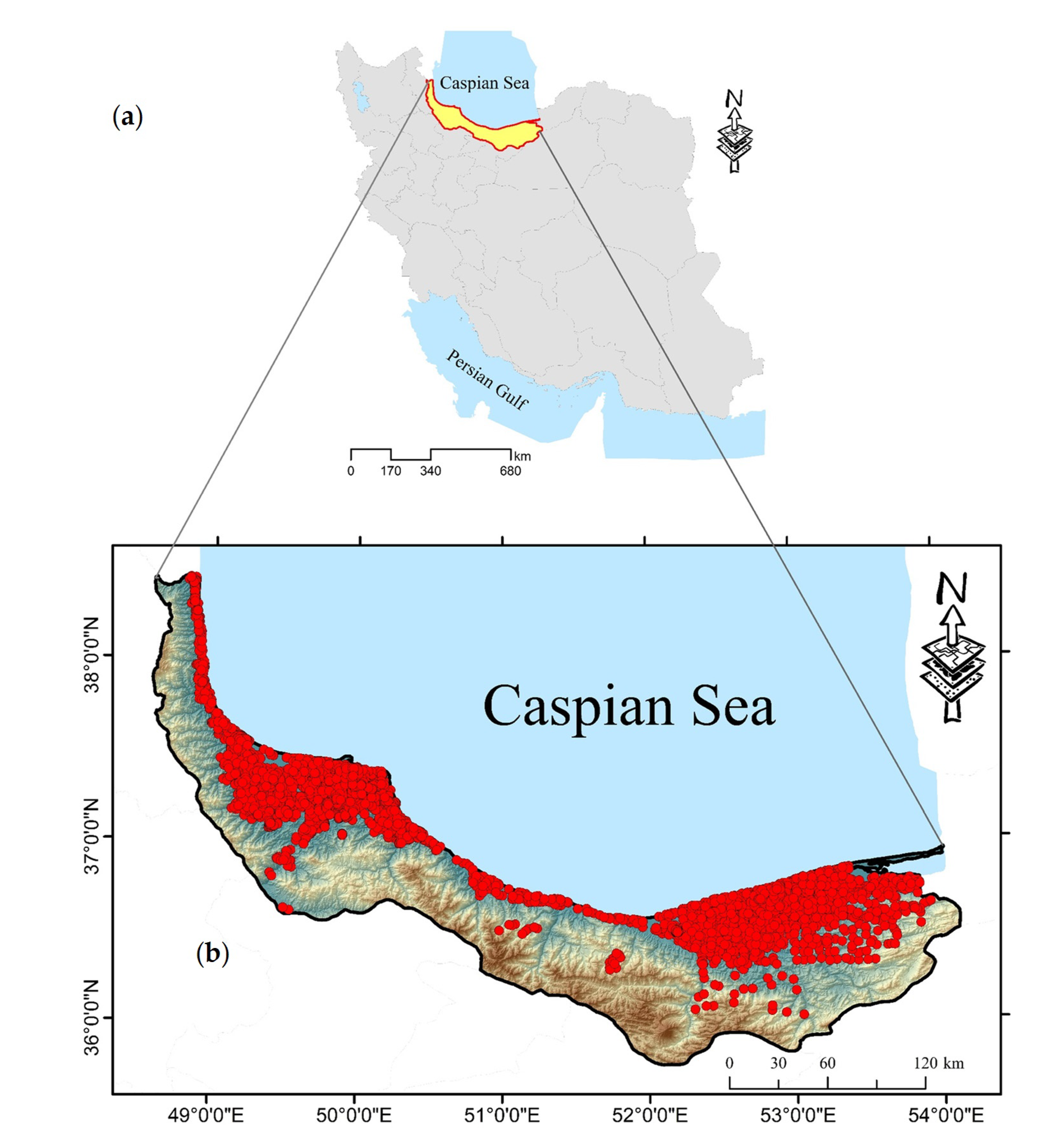
2.1. Study Area

The study area is located in the northern part of Iran and belongs to the provinces of Mazandaran and Guilan (Figure 1a) which cover an area of 37,850 km2. The region is covered by dense temperate deciduous forest and crop fields, while the northern part borders the Caspian Sea and the Alborz mountains. The climate is mild and humid with mean annual rainfall ranging from 879 to 1200 mm and reaching as high as 1900 mm in the Southwest of the study area. The precipitation increases with increasing elevation and is highest in the northwest of the study region along the Caspian Sea coast [33], Figure 1 and Figure 2). The region usually does not experience dryness [34]. The elevation varies between −27 and 5610 m above sea level. The geomorphology varies from high mountainous areas to lowlands along a south-north trajectory. The population is dense due to diverse natural resources and agricultural activities.

2.2. Soil Data

The soil samples were collected from various research projects. Most of these projects focused on agricultural fields under the supervision of the Soil Genesis and Classification Department of the Soil and Water Research Institute of Iran. A total of 6100 soil samples were collected from the surface layer (0–30 cm) and analyzed between 2000 and 2020 (Figure 1b). Sand, silt, and clay size fractions were measured using the hydrometer method [35] and soil textural class was determined based on the USDA textural classification system.
The soil samples represented a wide range of soil textures varying from clayey to very sandy soils (clay: C, clay loam: CL, loam: L, loamy sand: LS, sand: S, sandy clay loam; SCL, sandy loam: SL, silty clay: ZC, silty clay loam: ZCL, silt loam: ZL) with the clay content ranging from 0% to 70%, sand content ranging from 0% to 99%, and silt content ranging from 1% to 93%. Table 1 shows the percentage of each soil texture class, and Figure 2 illustrates the distribution of them in the original dataset. The high variation in soil texture could be related to the heterogeneity of parent materials, topography, morphology, erosion, land-use management, debris flows, and coastal sediments in the study area [36].

2.3. Balanced Data

Imbalanced data are often present in classes of many real-world observations. This problem sometimes causes poor performance of ML algorithms because the algorithms are biased to the majority classes and overlook the minority classes [37]. As a consequence, minority class instances are often misclassified as the majority ones [37]. Moreover, it has been shown most ML models overestimate the majority classes and underestimate the minority ones [38].
Several techniques have been developed to address the class imbalance issue. Among them, resampling techniques have been reported as effective solutions to deal with the problem by obtaining a more balanced data distribution [31,39,40,41]. A well-known and widely used resampling strategy is the synthetic minority oversampling technique, SMOTE [42]. The SMOTE algorithm uses an interpolation method to synthesize new examples from the existing examples, thus the minority class is over-sampled. In addition, this technique can be combined with a certain percentage of under-sampling of the majority class. To generate a synthetic sample, first, a random sample is selected from the minority class and its k nearest neighbors are found. Then, one of the randomly selected neighbors is chosen and a synthetic sample is generated at a point that is randomly selected between the two samples in feature space.

2.4. Environmental Covariates

In DSM, soil properties and classes are usually represented by environmental variables that are used as surrogates for soil forming factors including climate, relief, parent material, organisms, and time [16]. These environmental variables can be extracted from different sources such as remote sensing images, digital elevation models (DEMs), climatic maps, and legacy soil maps. Here, environmental covariates were extracted from remotely sensed images, DEMs, and bioclimatic data (Table 2). Remotely sensed data mostly represent organisms and parent materials while terrain-based data mostly represent the relief factor. Since different soils show different spectral behavior, spectral bands and their combinations have been used successfully in DSM to model and map soil properties and classes. Remotely sensed data including spectral bands and their combination as indices, were extracted from Landsat 8, Sentinel 2, and MODIS images. There are several terrain attributes that can be extracted from DEMs which are directly or indirectly relevant to soil classes. Terrain-based attributes were obtained from a DEM with 30 m spatial resolution.
Climate is one of the most important factors controlling soil and vegetation variations. Several climatic parameters can be used in DSM to model soil classes and/or properties. Bioclimatic variables (Table 2), which are derived from the monthly temperature and rainfall data, are useful variables in ecological modeling. They represent annual and seasonal trends in climatic parameters, as well as extreme climatic conditions. There are 19 bioclimatic variables available at https://www.worldclim.org (accessed on 29 August 2021) which were used in this research.
One disadvantage of ML algorithms is that, unlike geostatistical techniques, the spatial trends in the data cannot be included in the modeling process, therefore the predictions may contain spatial bias [25,43]. Several solutions have been proposed to deal with this issue. For example, it is proposed that including x and y coordinates and distances to the corners and middle of the study area in ML modeling can help resolve this issue [31,44]. Another proposed approach is calculating data layers with buffer distances to each soil observation and then using these layers as covariates [25]. Here, to take the spatial trend into account in modeling soil textural classes, we used distance layers (Table 2). All covariate layers were resampled to a grid with a 30 meters resolution.

2.5. Machine Learning

To model soil textural classes, environmental covariates were used as inputs for a random forest (RF) model. RFs are ensemble learning algorithms used for both classification and regression tasks, and were first introduced by [45]. The algorithm uses a tree-based approach for learning and rather than a single decision tree being trained, several decision trees are trained. During the training phase, bootstrap samples are taken from the training data set and each sample is used to create and train a decision tree. Explanatory variables (here environmental covariates) are introduced into each tree and the target variable is then estimated. For regression problems, the estimations of all trees in the forest are averaged to obtain one single estimate of the target variable while, for the classification problems, the class with the majority vote is considered as the final prediction.
One advantage of RFs is that the algorithm provides the relative importance of the environmental covariates used in modeling. In tree-based algorithms, explanatory variables are used to split the decision nodes. The most important variables are used as splitting criteria at the root nodes, while less important variables are used at nodes further from the root node. Therefore, the farther the decision node is from the root node, the less important the variable is and vice versa. In other words, in a forest of decision trees, the most important variables are used at most root nodes as splitting criteria. Accordingly, researchers [46] developed a method called minimal depth (MD) that simply determines variable importance by the position of the variables in the decision trees and thus, is based on the decision tree structures. If the mean minimal depth (MMD) for a variable is small, then a large number of observations are divided into groups on the basis of this variable.

2.6. Accuracy Assessment

A 10 k-fold cross-validation strategy was employed to evaluate the RF model performance for modeling soil textural classes on both balanced and imbalanced datasets. To perform the validation, the dataset was divided into k folds and at each run, k-1 folds were used to train and the remaining fold was used to validate the model. This process repeats k times; thus, all folds were used for both training and validating the model.
Five validation statistics, including overall accuracy (OA), the kappa index (K-index), precision, recall, and F-score from a confusion matrix were calculated (Equations (1)–(5)). In brief, OA is the ratio of all soil textural classes which classified correctly compared to all the data used. A higher overall accuracy indicates a high model performance. The kappa index is a robust index that considers the probability that a class is classified by chance [47]. It simply measures the proportion of all possible cases of presence or absence that are correctly predicted by a model after accounting for chance predictions. A higher kappa index indicates a high model performance [48,49]. Precision is the proportion of correctly classified predicted instances, recall is the proportion of those instances that are correctly classified, and the F-score is the harmonic mean of precision and recall (Equations (1)−(5)). A confusion matrix is a table that represents the relationship between the positive class and negative class predictions [50]. In other words, it determines which of the following categories the predictions fall into: true positive (TP), true negative (TN), false positive (FP), and false negative (FN).
OA = TP + TN TP + TN + FP + FN
K - index = 1 1 OA 1 P e
precision = TP TP + FP
recall = TP TP + FN
F - score = 2 × precision × recall recall + precision = 2 × TP 2 × TP + FP + FN
where P e is the expected agreement between the classifier and the true values.

3. Results and Discussion

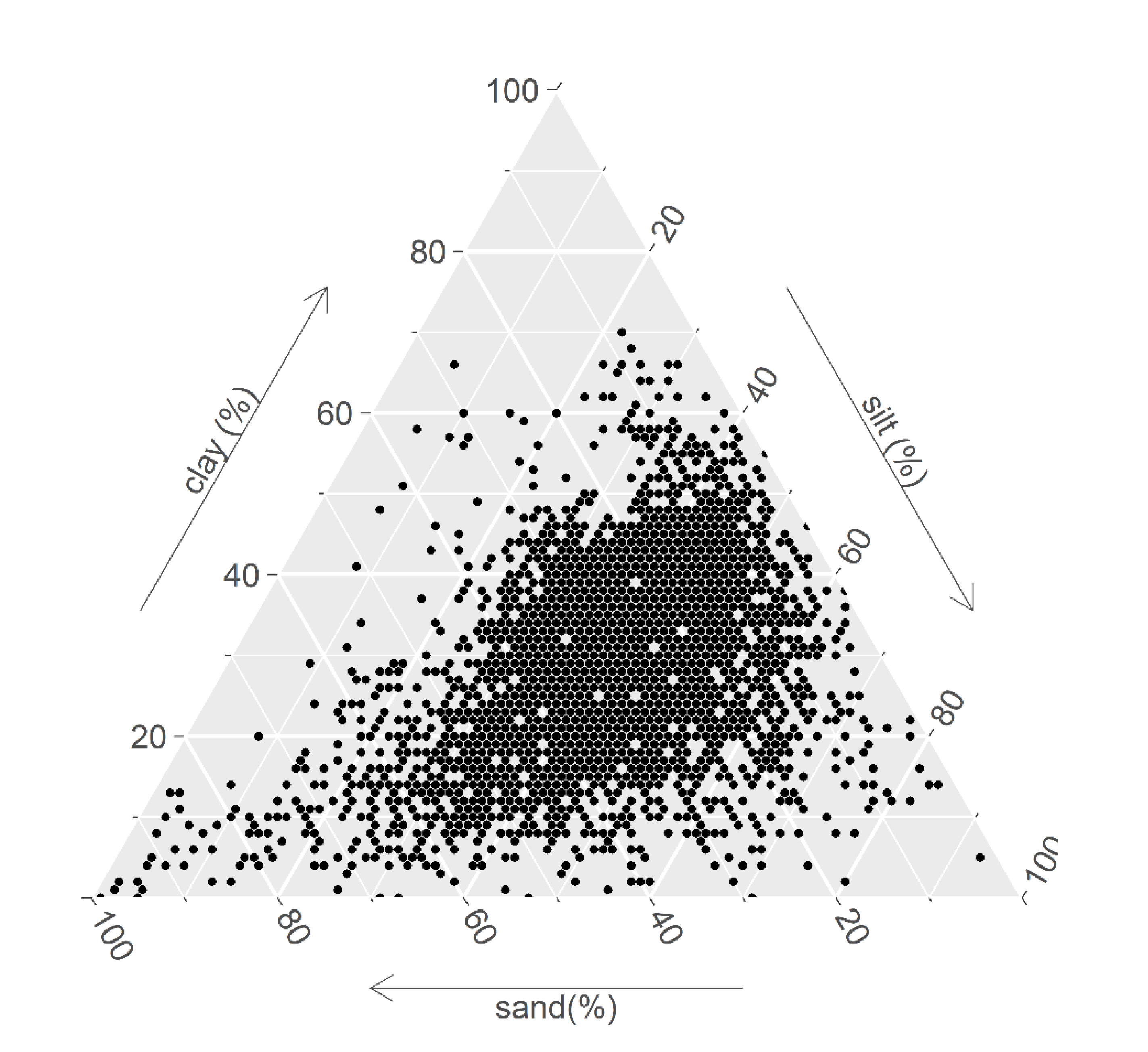
3.1. Balanced and Imbalanced Datasets

The dataset was treated using balanced and imbalanced approaches to investigate how these influenced predictions. The number of samples for each soil textural class varied due to different numbers of observations in each class for the imbalanced dataset (Figure 3a). The data were randomly generated and equally divided (600 samples) within the soil textural classes to produce a balanced dataset (Figure 3b). The majority of classes were L (1529 observations) and CL (1487 observations) and these accounted for more than half of the imbalanced dataset (Figure 3a). Balancing the distribution of soil textural classes causes the oversampling in minority soil texture classes (e.g., LS, S, and ZC). However, the number of observations for the C, CL, L, and ZL classes decreased due to under-sampling. The changes in the number of soil textural classes through resampling treatments are shown in Figure 3.

3.2. Accuracy Assessment

Resampling with the SMOTE method increased OA, precision, K-index, recall value, and F-score compared to when the imbalanced dataset was used (Table 3). Results clearly indicate that the RF model was trained better by the balanced SMOTE resampled dataset than the original imbalanced dataset. Using balanced data increased the overall accuracy by 15% (improving from 44% to 59%) and the kappa index by 22% (improving from 0.3 to 0.52) compared to the imbalanced dataset (Table 3). According to [51], this value of the kappa index represents a substantial agreement between observations and predictions. By balancing the data, model precision for all textural classes showed an increasing trend except for SCL. Recall values indicated that when balanced textural classes were modeled by RFs, more classes were classified correctly (except for CL). The number of samples in each textural class showed a significant effect on the number of correctly classified classes (i.e., recall values). In other words, the smaller the number of samples in an imbalanced textural class, the greater the number of correctly classified samples in the balanced data. As can be seen in Table 3, classes with a few samples in the imbalanced dataset (i.e., LS, S, SCL, and SL) showed the highest increase in recall values after balancing (17.75, 53, 6.37, and 7.37%, respectively). Recall values also indicate that minority classes that were overlooked (S) or misclassified as majority classes (LS, SCL, and SL) when trained using the imbalanced dataset, were well predicted with recall values of 0.51 to 0.71 using the balanced dataset (Table 3). A similar trend was observed for the F-scores.
To our knowledge, in previous studies, only soil taxonomic classes have been studied as imbalanced datasets. In line with our findings, a positive relationship has been reported between the sample size and the prediction accuracy of individual soil classes in previous studies [7,52]. A relatively poor prediction accuracy for soil taxonomic classes with a small sample size has been reported in central Iran [53]. In modeling reference soil groups of Iran, it was indicated that reference soil groups with a larger number of samples were modeled more accurately by ML algorithms than classes with small sample sizes [36]. Researchers [54] used 11 predictive models to model USDA subgroups and showed that over-sampling of the minority classes resulted in an increase in OA for some of the models. In addition, they indicated that the overlooked minority classes in the imbalanced data were predicted by over-sampling and were evident in the final map. Silva et al. [55] tested three models for predicting soil taxonomic classes in the USDA classification system. They found that the RF model which included additional sampling based on photo-interpretation showed the best performance among the studied models. Sharififar et al. [32] used Markov chain random fields in combination with an oversampling strategy to model USDA soil great groups in northwestern Iran. They showed, regardless of the models, that imbalanced data on soil taxonomic classes could affect both prediction and simulation model outputs. Moreover, they reported an improvement in the performance of the RF model after applying resampling techniques.

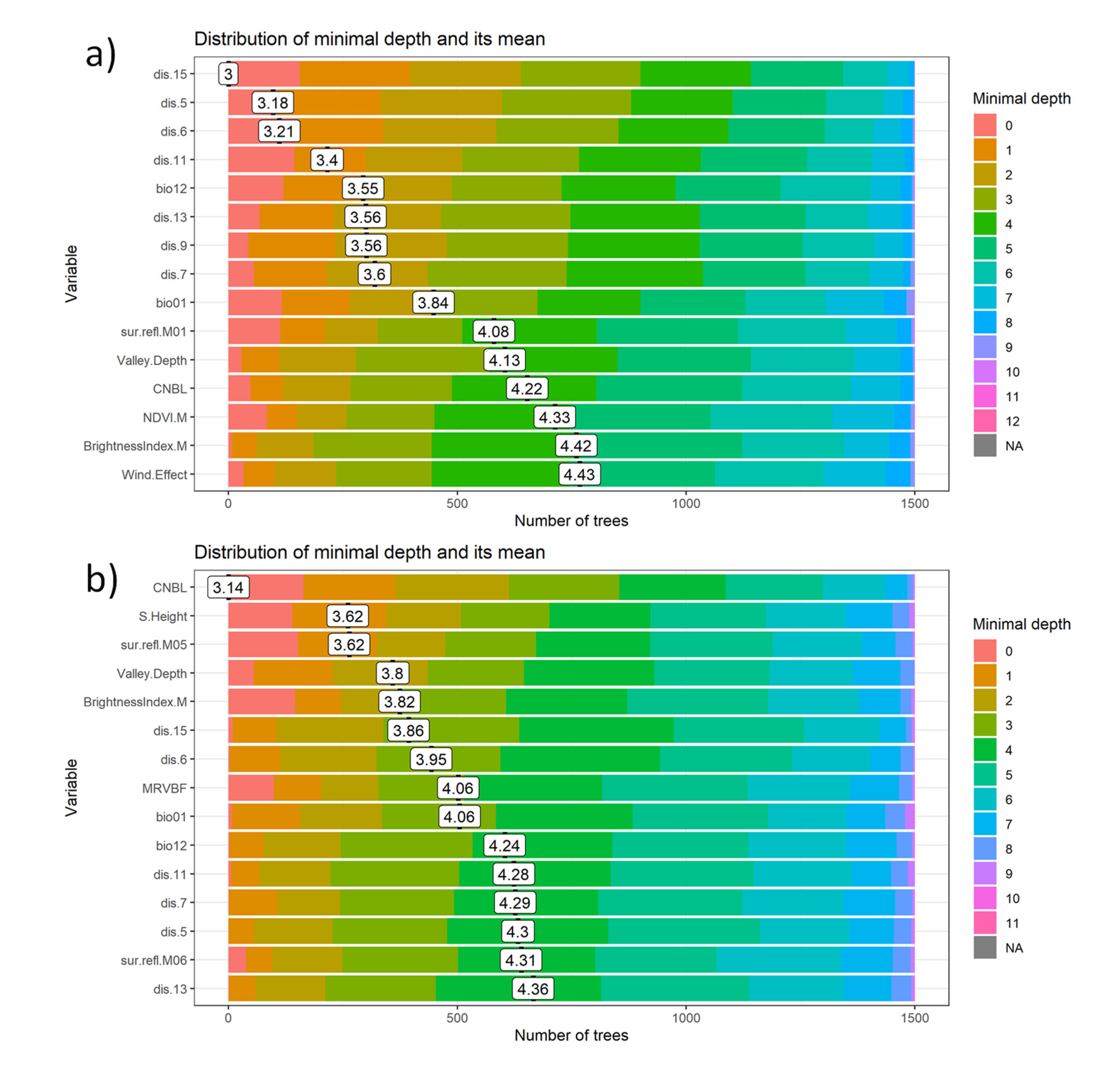
3.3. Covariate Importance

Minimal depths and their mean for only the 15 most important environmental covariates used for modeling imbalanced and balanced soil textural classes are presented in Figure 4. Covariates with lower MMD values show higher abilities for predicting soil textural classes. Distance layers showed a significant contribution in modeling soil textural classes when the imbalanced dataset was used (Figure 4a). This shows the high importance of spatial variance and uncertainties in the predictions, which emerging from different number of classes and also distances in the imbalance dataset.
For the balanced data (Figure 4b), the contribution of covariates is different from that obtained for the imbalanced data (Figure 4a). In contrast to when the imbalanced data were used, terrain attributes and remotely sensed data were more important in predicting textural classes than distance layers when the balanced data was used (Figure 4b). The contribution of terrain-based attributes and remotely sensed data to soil texture variations has been reported in several studies [28,56,57,58]. Remotely sensed data are used in DSM mostly as proxies of parent materials and organisms/vegetation [59] which significantly affect the spatial distribution of soil texture. Terrain attributes affect water distribution and redistribution, soil erosion and deposition [60,61], and consequently soil texture. Distance layers and bioclimatic variables showed lower contributions for predicting soil textural class variations after applying the resampling strategy.
Results showed that the most important variables varied significantly when the balanced dataset was used compared to when the original dataset was used (Figure 4a,b). This is because when unbalanced data are used, the number of samples in minority classes and the associated covariates is few, and therefore, these covariates were not considered important explanatory variables by the RF algorithm. In other words, in minority soil classes, the covariate variations do not usually cover soil variations completely. Therefore, by over-sampling, the minority classes and consequently increasing the number of associated covariates, the relative importance of some covariates in predicting textural classes may increase. Overall, results indicate that balancing can increase the relative importance of some important covariates that are overlooked by the model due to the small number of observations in certain textural classes.
A problem which may arise from an imbalanced dataset is selecting the optimal feature subsets. Because a subset of features that is optimal for modeling a minority class may not be optimal for the majority class and vice versa. Therefore, the selected features can be significantly affected when a dataset with imbalanced class distribution is used. This is an important issue that is not considered by traditional feature selection methods and may lead to poor prediction for minority class examples [62,63]. By applying balancing techniques, the results of feature selection algorithms will not depend on the class distribution. However, we should acknowledge that the inadequate testing of governing soil forming factors and their influence on soil texture variations in the region cannot be directly inferred from the feature importance analysis. Wadoux et al. [64] stated that pedological knowledge discovery based on ML is to be treated with caution. This is mainly because the predictive power of the features is based on the ML models and accuracy metrics (e.g., RMSE, ME, and R2).

3.4. Predicted Maps

The maps of soil textural classes produced using RF models based on the balanced and imbalanced datasets are shown in Figure 5. Ten main USDA soil texture classes were identified in the study area. Importantly, the main differences between the two maps (Figure 5a,b) are because of the using balanced and imbalanced data in modelling approach. For example, the predominant soil textures identified when using imbalanced data were L and CL (Figure 5a), while SL prevailed in the areas with elevations higher than 500 m above level using balanced data (Figure 5b). The visual assessment of these maps further shows that the imbalanced data was best at predicting the distribution of the L and CL soil textures which agrees with the observed dataset shown in Figure 2. This result was expected because the greatest number of the observations were allocated in the two soil classes of L and CL (Figure 2), leading to decrease of the RF power to detect the other soil texture classes (e.g., SL). Nevertheless, the RF trained by balanced data performed better compared to that obtained by imbalanced data. Several other studies have reported that resampling techniques, i.e., over and under-sampling, improved classification accuracy [32,65,66].
We should consider the main purpose of resampling techniques is not improving the accuracy of models but enhancing the predicted maps, particularly minority soil classes. Comparing the maps indicated that soil textures containing significant amounts of sand including LS (coded in dark blue), S (coded in pale blue), and SCL (coded in pale green) are almost excluded from the map produced by the RF model using imbalanced data. While the area with sandy soils is small, it is important to identify it because light-textured soils require specific management strategies for agricultural production and other land uses. Compared to heavy soil textures, sandy soils have coarse particles. According to the balanced data, the light soil textures were particularly found in the coastal areas which were covered by sand dunes, while the imbalanced approach could not delineate these areas properly. This finding again suggests that balanced training data exhibit better classification rates in comparison to the imbalanced data.
Furthermore, both approaches showed that the soil texture in the eastern part of the study area had silty soil texture classes. This could be related to regional-scale loess-paleosol deposits which developed due to wind erosion during Pleistocene climate change when there were relatively dry phases [67]. In general, the clayey soil textures are mostly located in the areas under rice cultivation where fine soil particles have been moved by floods from highlands to lowlands in the distant past or have originated from in situ weathering of parent materials with a fine particles size.

4. Conclusions

This study provided some insight into soil texture mapping with imbalanced and balanced datasets. The effect of imbalanced classes in the training dataset when using RF models and employing DSM approaches was the main focus of this study. The effects of balance and imbalance were investigated through pre-treatment of the data. The data treatment with under- and over-sampling improved the prediction of the minority S and LS soil texture classes.
The imbalanced dataset achieved relatively poor accuracies compared to the balanced approach, but no classes were lost. The increase in the accuracy of predictions was substantial with accuracy increases ranging from 9% to 50%, except for SCL whose accuracy decreased by more than half. Zero correct predictions of sand as the most minor class were mainly due to the small number of observations in the dataset.
The RF model was found to produce reasonable outputs according to all accuracy metrics when the SMOTE dataset resampling method was used, but could not detect important covariates in the imbalanced dataset and therefore variation of minority soil classes was not entirely represented. Distance layers and climate showed a significant contribution in modeling soil textural classes in terms of MMD when imbalanced and balanced datasets were used, respectively.
Based on the results, balancing the dataset is a promising alternative to the conventional imbalanced approach of soil textural mapping since computation is not complicated. However, further investigation is needed to improve the accuracy of the applied novel models. Precise prediction of static soil properties in the form of spatial maps is very important for decision-makers. These maps have valuable information to determine appropriate soil management strategies which leads to more sustainable use of available resources.

Author Contributions

Conceptualization, N.D. and R.T.-M.; methodology, S.M., B.D.K., A.A.-C., M.E., R.K., R.T.-M. and T.S.; software, S.M., B.D.K., A.A.-C., M.E., R.K., R.T.-M., T.S. and A.H.M.; validation, S.M., B.D.K., N.D., A.A.-C., M.E., R.K., R.T.-M., T.S. and A.H.M.; formal analysis, S.M., B.D.K., A.A.-C., M.E., R.K., R.T.-M., T.S. and A.H.M.; investigation, S.M., B.D.K., A.A.-C., M.E., R.K., R.T.-M., T.S. and A.H.M.; resources, N.D., A.A.-C., M.E., R.K., R.T.-M., T.S. and A.H.M.; data curation, S.M., B.D.K., A.A.-C., M.E., R.K., R.T.-M., T.S. and A.H.M.; writing—original draft preparation, S.M., B.D.K., N.D., A.A.-C., M.E., R.K., R.T.-M., T.S. and A.H.M.; writing—review and editing, S.M., B.D.K., N.D., A.A.-C., M.E., R.K., R.T.-M., T.S. and A.H.M.; visualization, A.A.-C., M.E., R.K., R.T.-M., T.S. and A.H.M.; supervision, N.D., A.A.-C., M.E., R.K., R.T.-M., T.S. and A.H.M.; project administration, N.D., A.A.-C., M.E., R.K., R.T.-M., T.S. and A.H.M. All authors have read and agreed to the published version of the manuscript.

Funding

Ruhollah Taghizadeh-Mehrjardi and Thomas Scholten have been supported by the Deutsche Forschungsgemeinschaft (DFG, German Research Foundation) under Germany’s Excellence Strategy—EXC number 2064/1—Project number 390727645, and collaborative research center SFB 1070 ‘ResourceCultures’—Project number 215859406.

Institutional Review Board Statement

Not applicable.

Informed Consent Statement

Not applicable.

Data Availability Statement

The data presented in this study are available on request from the corresponding author. The data are not publicly available due to privacy restrictions.

Acknowledgments

The authors would like to thank the Soil and Water Research Institute (SWRI) for providing opportunities for this research. Ruhollah Taghizadeh-Mehrjardi and Thomas Scholten have been supported by the Deutsche Forschungsgemeinschaft (DFG, German Research Foundation) under Germany’s Excellence Strategy—EXC number 2064/1—Project number 390727645, and collaborative research center SFB 1070 ‘ResourceCultures’—Project number 215859406.

Conflicts of Interest

The authors declare no conflict of interest.

References

  1. Yolcubal, I.; Brusseau, M.L.; Artiola, J.F.; Wierenga, P.; Wilson, L.G. Environmental Physical Properties and Processes. In Environmental Monitoring and Characterization; Elsevier: Amsterdam, The Netherlands, 2004; pp. 207–239. ISBN 978-0-12-064477-3. [Google Scholar]
  2. Soil Survey Staff. Keys to Soil Taxonomy, 12th ed.; NRCS-USDA: Washington, DC, USA, 2014. [Google Scholar]
  3. USDA. USDA. USDA Textural Soil Classification. In Soil Mechanics Level I Module 3; United States Department of Agriculture, National Employee Staff, Soil Conservation Service: Washington, DC, USA, 1987. [Google Scholar]
  4. Borrelli, P.; Paustian, K.; Panagos, P.; Jones, A.; Schütt, B.; Lugato, E. Effect of Good Agricultural and Environmental Conditions on Erosion and Soil Organic Carbon Balance: A National Case Study. Land Use Policy 2016, 50, 408–421. [Google Scholar] [CrossRef]
  5. Gomes, L.C.; Faria, R.M.; de Souza, E.; Veloso, G.V.; Schaefer, C.E.G.R.; Filho, E.I.F. Modelling and Mapping Soil Organic Carbon Stocks in Brazil. Geoderma 2019, 340, 337–350. [Google Scholar] [CrossRef]
  6. Liu, F.; Zhang, G.-L.; Song, X.; Li, D.; Zhao, Y.; Yang, J.; Wu, H.; Yang, F. High-Resolution and Three-Dimensional Mapping of Soil Texture of China. Geoderma 2020, 361, 114061. [Google Scholar] [CrossRef]
  7. Hengl, B.D.; Heuvelink, T.; Kempen, G.; Mulder, B.; Olmedo, T.; Poggio, G.; Ribeiro, L.; Thine, E.; Omuto, C.; Yigini, Y. Soil Organic Carbon Mapping Cookbook; FAO: Rome, Italy, 2017; p. 180. [Google Scholar]
  8. Mahmoudzadeh, H.; Matinfar, H.R.; Taghizadeh-Mehrjardi, R.; Kerry, R. Spatial Prediction of Soil Organic Carbon Using Machine Learning Techniques in Western Iran. Geoderma Reg. 2020, 21, e00260. [Google Scholar] [CrossRef]
  9. Arrouays, D.; Grundy, M.G.; Hartemink, A.E.; Hempel, J.W.; Heuvelink, G.B.M.; Hong, S.Y.; Lagacherie, P.; Lelyk, G.; McBratney, A.B.; McKenzie, N.J.; et al. GlobalSoilMap. In Advances in Agronomy; Elsevier: Amsterdam, The Netherlands, 2014; Volume 125, pp. 93–134. ISBN 978-0-12-800137-0. [Google Scholar]
  10. Adhikari, K.; Kheir, R.B.; Greve, M.B.; Bøcher, P.K.; Malone, B.P.; Minasny, B.; McBratney, A.B.; Greve, M.H. High-Resolution 3-D Mapping of Soil Texture in Denmark. Soil Sci. Soc. Am. J. 2013, 77, 860–876. [Google Scholar] [CrossRef]
  11. ViscarraRossel, R.A.; Chen, C.; Grundy, M.J.; Searle, R.; Clifford, D.; Campbell, P.H. The Australian Three-Dimensional Soil Grid: Australia’s Contribution to the GlobalSoilMap Project. Soil Res. 2015, 53, 845. [Google Scholar] [CrossRef] [Green Version]
  12. Mulder, V.L.; Lacoste, M.; Richer-de-Forges, A.C.; Arrouays, D. GlobalSoilMap France: High-Resolution Spatial Modelling the Soils of France up to Two Meter Depth. Sci. Total Environ. 2016, 573, 1352–1369. [Google Scholar] [CrossRef]
  13. Padarian, J.; Minasny, B.; McBratney, A.B. Chile and the Chilean Soil Grid: A Contribution to GlobalSoilMap. Geoderma Reg. 2017, 9, 17–28. [Google Scholar] [CrossRef]
  14. Ramcharan, A.; Hengl, T.; Nauman, T.; Brungard, C.; Waltman, S.; Wills, S.; Thompson, J. Soil Property and Class Maps of the Conterminous United States at 100-Meter Spatial Resolution. Soil Sci. Soc. Am. J. 2018, 82, 186–201. [Google Scholar] [CrossRef] [Green Version]
  15. Tóth, B.; Weynants, M.; Nemes, A.; Makó, A.; Bilas, G.; Tóth, G. New Generation of Hydraulic Pedotransfer Functions for Europe: New Hydraulic Pedotransfer Functions for Europe. Eur. J. Soil Sci. 2015, 66, 226–238. [Google Scholar] [CrossRef]
  16. McBratney, A.B.; Mendonça Santos, M.L.; Minasny, B. On Digital Soil Mapping. Geoderma 2003, 117, 3–52. [Google Scholar] [CrossRef]
  17. Li, M.; Wijewardane, N.K.; Ge, Y.; Xu, Z.; Wilkins, M.R. Visible/near Infrared Spectroscopy and Machine Learning for Predicting Polyhydroxybutyrate Production Cultured on Alkaline Pretreated Liquor from Corn Stover. Bioresour. Technol. Rep. 2020, 9, 100386. [Google Scholar] [CrossRef]
  18. Hamel, Z.; Ababou, A.; Saidi, D.; Kemassi, A. Evaluation of Soil Aggregate Stability in Algerian Northwestern Soils Using Pedotransfer Functions and Artificial Neural Networks. Acta Ecol. Sin. 2021, 41, 235–242. [Google Scholar] [CrossRef]
  19. Singh, G.; Panda, R.K.; Bisht, D.S. Improved Generalized Calibration of an Impedance Probe for Soil Moisture Measurement at Regional Scale Using Bayesian Neural Network and Soil Physical Properties. J. Hydrol. Eng. 2021, 26, 04020068. [Google Scholar] [CrossRef]
  20. Elbisy, M.S. Support Vector Machine and Regression Analysis to Predict the Field Hydraulic Conductivity of Sandy Soil. KSCE J. Civ. Eng. 2015, 19, 2307–2316. [Google Scholar] [CrossRef]
  21. Sihag, P.; Tiwari, N.K.; Ranjan, S. Support Vector Regression-Based Modeling of Cumulative Infiltration of Sandy Soil. ISHJ. Hydraul. Eng. 2018, 26, 1–7. [Google Scholar] [CrossRef]
  22. Kovačević, M.; Bajat, B.; Gajić, B. Soil Type Classification and Estimation of Soil Properties Using Support Vector Machines. Geoderma 2010, 154, 340–347. [Google Scholar] [CrossRef]
  23. Barman, U.; Choudhury, R.D. Soil Texture Classification Using Multi Class Support Vector Machine. Inf. Process. Agric. 2020, 7, 318–332. [Google Scholar] [CrossRef]
  24. Martin, M.P.; Lo Seen, D.; Boulonne, L.; Jolivet, C.; Nair, K.M.; Bourgeon, G.; Arrouays, D. Optimizing Pedotransfer Functions for Estimating Soil Bulk Density Using Boosted Regression Trees. Soil Sci. Soc. Am. J. 2009, 73, 485–493. [Google Scholar] [CrossRef]
  25. Hengl, T.; Nussbaum, M.; Wright, M.N.; Heuvelink, G.B.M.; Gräler, B. Random Forest as a Generic Framework for Predictive Modeling of Spatial and Spatio-Temporal Variables. PeerJ 2018, 6, e5518. [Google Scholar] [CrossRef]
  26. Dharumarajan, S.; Hegde, R. Digital Mapping of Soil Texture Classes Using Random Forest Classification Algorithm. Soil Use Manag. 2022, 38, 135–149. [Google Scholar] [CrossRef]
  27. Szabó, B.; Szatmári, G.; Takács, K.; Laborczi, A.; Makó, A.; Rajkai, K.; Pásztor, L. Mapping Soil Hydraulic Properties Using Random-Forest-Based Pedotransfer Functions and Geostatistics. Hydrol. Earth Syst. Sci. 2019, 23, 2615–2635. [Google Scholar] [CrossRef] [Green Version]
  28. Kardani, N.; Bardhan, A.; Gupta, S.; Samui, P.; Nazem, M.; Zhang, Y.; Zhou, A. Predicting Permeability of Tight Carbonates Using a Hybrid Machine Learning Approach of Modified Equilibrium Optimizer and Extreme Learning Machine. Acta Geotech. 2022, 17, 1239–1255. [Google Scholar] [CrossRef]
  29. Provost, F. Machine Learning from Imbalanced Data Sets 101. In Proceedings of the AAAI’2000 Workshop on Imbalanced Data Sets, Austin, TX, USA, 31 July 2000; Volume 68, pp. 1–3. [Google Scholar]
  30. Zhu, B.; Baesens, B.; vandenBroucke, S.K.L.M. An Empirical Comparison of Techniques for the Class Imbalance Problem in Churn Prediction. Inf. Sci. 2017, 408, 84–99. [Google Scholar] [CrossRef] [Green Version]
  31. Abdi, L.; Hashemi, S. To Combat Multi-Class Imbalanced Problems by Means of Over-Sampling Techniques. IEEE Trans. Knowl. Data Eng. 2016, 28, 238–251. [Google Scholar] [CrossRef]
  32. Sharififar, A.; Sarmadian, F.; Minasny, B. Mapping Imbalanced Soil Classes Using Markov Chain Random Fields Models Treated with Data Resampling Technique. Comput. Electron. Agric. 2019, 159, 110–118. [Google Scholar] [CrossRef]
  33. Baaghideh, M.; Dadashi-Roudbari, A.; Beiranvand, F. Analysis of Precipitation Variation in the Northern Strip of Iran. Model. Earth Syst. Environ. 2020, 6, 567–574. [Google Scholar] [CrossRef]
  34. Ziarati, P.; Zendehdel, T.; Bidgoli, S.A. Nitrate Content in Drinking Water in Gilan and Mazandaran Provinces, Iran. J. Environ. Anal. Toxicol. 2014, 4, 1. [Google Scholar] [CrossRef] [Green Version]
  35. Gee, G.W.; Bauder, J.W. Particle Size Analysis. In Methods of Soil Analysis, Part 1 (Second Ed.), 9th ed.; Klute, A., Ed.; Soil Science Society of America: Madison, WI, USA, 1986; pp. 383–411. [Google Scholar]
  36. Taghizadeh-Mehrjardi, R.; Mahdianpari, M.; Mohammadimanesh, F.; Behrens, T.; Toomanian, N.; Scholten, T.; Schmidt, K. Multi-Task Convolutional Neural Networks Outperformed Random Forest for Mapping Soil Particle Size Fractions in Central Iran. Geoderma 2020, 376, 114552. [Google Scholar] [CrossRef]
  37. Fernández, A.; García, S.; Galar, M.; Prati, R.C.; Krawczyk, B.; Herrera, F. Dimensionality Reduction for Imbalanced Learning. In Learning from Imbalanced Data Sets; Springer International Publishing: Cham, Switzerland, 2018; pp. 227–251. ISBN 978-3-319-98073-7. [Google Scholar]
  38. Grunwald, S. Multi-Criteria Characterization of Recent Digital Soil Mapping and Modeling Approaches. Geoderma 2009, 152, 195–207. [Google Scholar] [CrossRef]
  39. Chawla, N.V.; Cieslak, D.A.; Hall, L.O.; Joshi, A. Automatically Countering Imbalance and Its Empirical Relationship to Cost. Data Min. Knowl. Disc. 2008, 17, 225–252. [Google Scholar] [CrossRef] [Green Version]
  40. Estabrooks, A.; Jo, T.; Japkowicz, N. A Multiple Resampling Method for Learning from Imbalanced Data Sets. Comput. Intell. 2004, 20, 18–36. [Google Scholar] [CrossRef] [Green Version]
  41. García, V.; Sánchez, J.S.; Martín-Félez, R.; Mollineda, R.A. Surrounding Neighborhood-Based SMOTE for Learning from Imbalanced Data Sets. Prog. Artif. Intell. 2012, 1, 347–362. [Google Scholar] [CrossRef] [Green Version]
  42. Chawla, N.V.; Bowyer, K.W.; Hall, L.O.; Kegelmeyer, W.P. SMOTE: Synthetic Minority Over-Sampling Technique. J. Artif. Intell. Res. 2002, 16, 321–357. [Google Scholar] [CrossRef]
  43. Møller, A.B.; Beucher, A.M.; Pouladi, N.; Greve, M.H. Oblique Geographic Coordinates as Covariates for Digital Soil Mapping. SOIL 2020, 6, 269–289. [Google Scholar] [CrossRef]
  44. Behrens, T.; Schmidt, K.; ViscarraRossel, R.A.; Gries, P.; Scholten, T.; MacMillan, R.A. Spatial Modelling with Euclidean Distance Fields and Machine Learning: Spatial Modelling with Euclidean Distance Fields. Eur. J. Soil Sci. 2018, 69, 757–770. [Google Scholar] [CrossRef]
  45. Breiman, L. Random Forests. Mach. Learn. 2001, 45, 5–32. [Google Scholar] [CrossRef] [Green Version]
  46. Ishwaran, H.; Kogalur, U.B. Consistency of Random Survival Forests. Stat. Probab. Lett. 2010, 80, 1056–1064. [Google Scholar] [CrossRef] [PubMed] [Green Version]
  47. Behrens, T.; Zhu, A.-X.; Schmidt, K.; Scholten, T. Multi-Scale Digital Terrain Analysis and Feature Selection for Digital Soil Mapping. Geoderma 2010, 155, 175–185. [Google Scholar] [CrossRef]
  48. Brazil, I.N.P.E. Monitoramento da F/floresta Amaz6nica Brasileira por Satelite. Monit. Braz. Amazon For. Satel. 1999, 1999, 20011. [Google Scholar]
  49. da Silva, A.F.; Barbosa, A.P.; Zimback, C.R.L.; Landim, P.M.B.; Soares, A. Estimation of Croplands Using Indicator Kriging and Fuzzy Classification. Comput. Electron. Agric. 2015, 111, 1–11. [Google Scholar] [CrossRef]
  50. Lantz, B. Machine Learning with R: Expert Techniques for Predictive Modeling; Packt Publishing Ltd.: Birrmingham, UK, 2019. [Google Scholar]
  51. Landis, J.R.; Koch, G.G. An Application of Hierarchical Kappa-Type Statistics in the Assessment of Majority Agreement among Multiple Observers. Biom. 1977, 33, 363–374. [Google Scholar] [CrossRef]
  52. Brungard, C.W.; Boettinger, J.L.; Duniway, M.C.; Wills, S.A.; Edwards, T.C. Machine Learning for Predicting Soil Classes in Three Semi-Arid Landscapes. Geoderma 2015, 239–240, 68–83. [Google Scholar] [CrossRef] [Green Version]
  53. Jafari, A.; Finke, P.A.; VandeWauw, J.; Ayoubi, S.; Khademi, H. Spatial Prediction of USDA- Great Soil Groups in the Arid Zarand Region, Iran: Comparing Logistic Regression Approaches to Predict Diagnostic Horizons and Soil Types. Eur. J. Soil Sci. 2012, 63, 284–298. [Google Scholar] [CrossRef]
  54. Neyestani, M.; Sarmadian, F.; Jafari, A.; Keshavarzi, A.; Sharififar, A. Digital Mapping of Soil Classes Using Spatial Extrapolation with Imbalanced Data. Geoderma Reg. 2021, 26, e00422. [Google Scholar] [CrossRef]
  55. Silva, B.P.C.; Silva, M.L.N.; Avalos, F.A.P.; de Menezes, M.D.; Curi, N. Digital Soil Mapping Including Additional Point Sampling in Posses Ecosystem Services Pilot Watershed, Southeastern Brazil. Sci. Rep. 2019, 9, 13763. [Google Scholar] [CrossRef] [PubMed] [Green Version]
  56. Akpa, S.I.C.; Odeh, I.O.A.; Bishop, T.F.A.; Hartemink, A.E. Digital Mapping of Soil Particle-Size Fractions for Nigeria. Soil Sci. Soc. Am. J. 2014, 78, 1953–1966. [Google Scholar] [CrossRef] [Green Version]
  57. Taghizadeh-Mehrjardi, R.; Emadi, M.; Cherati, A.; Heung, B.; Mosavi, A.; Scholten, T. Bio-Inspired Hybridization of Artificial Neural Networks: An Application for Mapping the Spatial Distribution of Soil Texture Fractions. Remote Sens. 2021, 13, 1025. [Google Scholar] [CrossRef]
  58. Amirian-Chakan, A.; Minasny, B.; Taghizadeh-Mehrjardi, R.; Akbarifazli, R.; Darvishpasand, Z.; Khordehbin, S. Some Practical Aspects of Predicting Texture Data in Digital Soil Mapping. Soil Tillage Res. 2019, 194, 104289. [Google Scholar] [CrossRef]
  59. Malone, B.P.; Minasny, B.; McBratney, A.B. Using R for Digital Soil Mapping. In Progress in Soil Science; Springer International Publishing: Cham, Switzerland, 2017; ISBN 978-3-319-44325-6. [Google Scholar]
  60. Gallant, J.C.; Dowling, T.I. A Multiresolution Index of Valley Bottom Flatness for Mapping Depositional Areas: MULTIRESOLUTION VALLEY BOTTOM FLATNESS. Water Resour. Res. 2003, 39. [Google Scholar] [CrossRef]
  61. Umali, B.P.; Oliver, D.P.; Forrester, S.; Chittleborough, D.J.; Hutson, J.L.; Kookana, R.S.; Ostendorf, B. The Effect of Terrain and Management on the Spatial Variability of Soil Properties in an Apple Orchard. Catena 2012, 93, 38–48. [Google Scholar] [CrossRef]
  62. Tyagi, S.; Mittal, S. Sampling Approaches for Imbalanced Data Classification Problem in Machine Learning. In Proceedings of the ICRIC 2019, Jammu, India, March 2019; Singh, P.K., Kar, A.K., Singh, Y., Kolekar, M.H., Tanwar, S., Eds.; Lecture Notes in Electrical Engineering. Springer International Publishing: Cham, Switzerland, 2020; Volume 597, pp. 209–221. [Google Scholar]
  63. Kamal, A.H.M.; Zhu, X.; Pandya, A.; Hsu, S.; Narayanan, R. Feature Selection for Datasets with Imbalanced Class Distributions. Int. J. Soft. Eng. Knowl. Eng. 2010, 20, 113–137. [Google Scholar] [CrossRef]
  64. Wadoux, A.M.C.; Samuel-Rosa, A.; Poggio, L.; Mulder, V.L. A Note on Knowledge Discovery and Machine Learning in Digital Soil Mapping. Eur. J. Soil Sci. 2020, 71, 133–136. [Google Scholar] [CrossRef]
  65. Sáez, J.A.; Krawczyk, B.; Woźniak, M. Analyzing the Oversampling of Different Classes and Types of Examples in Multi-Class Imbalanced Datasets. Pattern Recognit. 2016, 57, 164–178. [Google Scholar] [CrossRef]
  66. Loyola-González, O.; Martínez-Trinidad, J.F.; Carrasco-Ochoa, J.A.; García-Borroto, M. Study of the Impact of Resampling Methods for Contrast Pattern Based Classifiers in Imbalanced Databases. Neurocomputing 2016, 175, 935–947. [Google Scholar] [CrossRef]
  67. Kehl, M.; Vlaminck, S.; Köhler, T.; Laag, C.; Rolf, C.; Tsukamoto, S.; Frechen, M.; Sumita, M.; Schmincke, H.-U.; Khormali, F. Pleistocene Dynamics of Dust Accumulation and Soil Formation in the Southern Caspian Lowlands—New Insights from the Loess-Paleosol Sequence at Neka-Abelou, Northern Iran. Quat. Sci. Rev. 2021, 253, 106774. [Google Scholar] [CrossRef]
Figure 1. Location of the study area within Iran (a) and location of the soil samples collected within the study area (b) plotted over a 90 m SRTM DEM showing variations in elevation.
Agronomy 12 02613 g001
Figure 2. Distribution of soil textural classes within the study area.
Agronomy 12 02613 g002
Figure 3. The number of observations in each soil textural class for (a) imbalanced and (b) balanced datasets (C: clay; CL: clay loam; L: loam; LS: loamy sand; S: sand; SCL: sandy clay loam; SL: sandy loam; ZC: silty clay; ZCL: silty clay loam; ZL: silt loam).
Agronomy 12 02613 g003
Figure 4. The MMD (mean minimal depth) of environmental covariates for predicting soil texture classes using the random forest method based on (a) imbalanced and (b) balanced datasets (dis.5, dis.15: Distance to different parts of the study area, bio01: Temperature, sur.refl: surface reflectance; Valley.Depth: Valley.Depth, CNBL: channel network based level, NDVI: normalized difference vegetation index, Wind.Effect: wind effect, S.Height: Slope.Height, MRVBF: multiresolution valley bottom flatness, bio12: Rainfall).
Agronomy 12 02613 g004
Figure 5. Spatial distribution of the most probable soil textural classes produced using: (a) RFs with imbalanced data and (b) RFs with balanced data in the southern Caspian Sea area of Northern Iran (C: clay; ZC: silty clay; ZCL: silty clay loam; SCL: sandy clay loam; CL: clay loam; ZL: silt loam; L: loam; S: sand; LS: loamy sand; SL: sandy loam).
Agronomy 12 02613 g005
Table 1. The percentages of soil texture classes in the original dataset.
Soil TextureCCLLLSSSCLSLZCZCLZL
Percentage (%) in the original dataset13/2724/4025/090/390/204/284/869/389/8111/21
C: clay; CL: clay loam; L: loam; LS: loamy sand; S: sand; SCL: sandy clay loam; SL: sandy loam ZC: silty clay; ZCL: silty clay loam; ZL: silt loam.
Table 2. Environmental covariates used for modelling soil textural classes.
Source CovariateAbbreviation
DEM Aspect-
Catchment areaCat.Area
Catchment slopeCat.Slope
Channel network-based levelCNBL
Channel network distance indexCNDI
Convergence indexCon.Index
Elevation-
Length-slope factorLS.Factor
Mid slope positionMid.Slope.P
Modified catchment areaM.Cat.Area
Multiresolution ridge top flatnessMRRTF
Multiresolution valley bottom flatnessMRVBF
Normalized heightN.Height
Plan curvaturePlan.Cur
Profile curvatureProf.Cur
Relative slope positionR.Slope.P
Slope heightSlope.Height
Slope-
Standard heightS.Height
Topographic wetness indexTWI
Total catchment areaTotal.Cat.Area
Valley depthValley.Depth
Wind effectWind.Effect
Remote sensing images aSentinel-2Sentinel-2 spectral bands (B2.S, B3.S, B4.S, B5.S, B6.S, B7.S, B8.S, B11.S, B12.S)
Normalized difference vegetation indexNDVI
Soil adjusted vegetation indexSAVI
Brightness indexBrightnessIndex
Clay indexClayIndex
Landsat 8Landsat 8 spectral bands (B2.L, B3.L, B4.L, B5.L, B6.L, B7.L, B10.L, B11.L)
NDVI, SAVI, brightness index, clay index
MODISMODIS spectral bands (B1.M, B2.M, B3.M, B4.M, B5.M, B6.M, B7.M)
NDVI, SAVI, brightness index, clay index
Bioclimatic data Rainfall
Temperature
Bio12
Bio01
Distance layers Distance to different parts of the study areadis.1, … dis.15
a S, L, and M letters indicate Sentinel, Landsat, and MODIS, respectively.
Table 3. Validation statistics calculated using the confusion matrix.
Soil Texture Imbalanced Balanced
PrecisionRecallF-ScorePrecisionRecallF-Score
C0.450.380.410.610.680.64
CL0.410.510.460.750.520.62
L0.460.600.520.750.590.66
LS0.150.040.070.300.710.42
S0.000.000.000.200.530.29
SCL0.560.080.140.250.510.33
SL0.290.080.130.360.590.45
ZC0.450.400.430.570.670.61
ZCL0.440.320.370.480.640.55
ZL0.460.350.400.530.540.53
C: clay; CL: clay loam; L: loam; LS: loamy sand; S: Sand; SCL: sandy clay loam; SL: sandy loam ZC: silty clay; ZCL: silty clay loam; ZL: silt loam.
Publisher’s Note: MDPI stays neutral with regard to jurisdictional claims in published maps and institutional affiliations.

