Article

The Segmented Colour Feature Extreme Learning Machine: Applications in Agricultural Robotics

1
School of Science & Technology, University of New England, Armidale, NSW 2351, Australia
2
College of Science & Engineering, Flinders University, Adelaide, SA 5042, Australia
3
Strategic Research Initiatives, University of New England, Armidale, NSW 2351, Australia
4
Precision Agriculture Research Group, University of New England, Armidale, NSW 2351, Australia
5
Food Agility Cooperative Research Centre Ltd., 81 Broadway, Ultimo, NSW 2007, Australia
*
Author to whom correspondence should be addressed.
Agronomy 2021, 11(11), 2290; https://doi.org/10.3390/agronomy11112290
Submission received: 11 October 2021 / Revised: 3 November 2021 / Accepted: 8 November 2021 / Published: 12 November 2021
(This article belongs to the Special Issue Data-Driven Agricultural Innovations)

Abstract

:
This study presents the Segmented Colour Feature Extreme Learning Machine (SCF-ELM). The SCF-ELM is inspired by the Extreme Learning Machine (ELM) which is known for its rapid training and inference times. The ELM is therefore an ideal candidate for an ensemble learning algorithm. The Colour Feature Extreme Learning Machine (CF-ELM) is used in this study due to its additional ability to extract colour image features. The SCF-ELM is an ensemble learner that utilizes feature mapping via k-means clustering, a decision matrix and majority voting. It has been evaluated on a range of challenging agricultural object classification scenarios including weed, livestock and machinery detection. SCF-ELM model performance results were excellent both in terms of detection, 90 to 99% accuracy, and also inference times, around 0.01(s) per image. The SCF-ELM was able to compete or improve upon established algorithms in its class, indicating its potential for remote computing applications in agriculture.

1. Introduction

Fast and accurate object detection is essential in many machine vision applications, particularly agricultural robotics. Due to processor and operational requirements, there is often a trade off between detection accuracy and processing speeds. Agricultural applications often opt for a statistical approaches to classification, including multivariant data analysis [1], principal componet analysis [2], template matching [3] and random forrest [4]. These implementations typically rely on a reduced set of attributes within a controlled environment. This is efficient and well suited to the application area, but has the potential for large numbers of false positives and/or false negatives in inconsistent terrain, which includes pastures for livestock. The Support Vector Machine (SVM) has shown promise in this space as a highly optimised solution [5], but still suffers from the proliferation of support vectors [6]. Object detection methods, including artificial neural networks (ANN) for deep learning allow higher levels of sophistication and can be utilised for complex environments [7]. Neural networks however, have long training phases and can be computationally intensive. This limits an ANN’s ability to calibrate and provide feedback in an remote environment, this is exemplified in remote devices that require the preservation of battery or have hardware limitations [8]. To overcome the training times and to improve classification of a shallow network, Huang et al. [9] proposed the Extreme Learning Machine (ELM). The ELM has a much faster training phase than other more common ANNs, where, instead of a long gradient decent based approach such as the back propagation algorithm [10], the ELM uses the pseudo inverse of its hidden layer output to analytically determine its output weights. Using this method the ELM is trained analytically in one calculation rather than a long iterative process. Another drawback of a standard ANN is that it typically uses grey-scale inputs to determine the output values and hence only grey-scale images can be used in training and testing. Colour however is not sensitive to adjustments in scale, size and location [11] and can provide key cues to object detection. To overcome these challenges Sadgrove et al [12] proposed the Colour Feature Extreme Learning Machine (CF-ELM) which uses the architecture of the ELM, but has a partially connected hidden layer with one section for each colour band and a fully connected output layer, allowing the CF-ELM to analytically determine its output weights and with the added information of colour. The CF-ELM has shown promise as a fast and accurate approach to real-time remote classification. This makes it an ideal choice for fast detection, however, the random neuron weights result in inconsistencies in results each time it is train [13]. To improve consistency in neural networks a large amount of hidden neurons are often used, where the ideal number of neurons is purported to be some where between the number of inputs and outputs [14]. The Multiple Expert Colour Feature Extreme Learning Machine (MEC-ELM) improved the consistency on low resolution images by using a small number of CF-ELMS trained on different sets of images [15]. The MEC-ELM however, did not take into account the change in orientation of objects for objects with consistent feature sets, such as animals and vehicles. The proposed SCF-ELM will utilise k-means for fast feature mapping, this will allow features to be mapped consistently to individual classifiers. It is hypothesized that by training unique features on individual classifiers, that this will improve overall performance of an ensemble, an equal k-means algorithm is proposed for fast convergence. The SCF-ELM will be trained using quasi-pseudo random weights, utilise a decision matrix and use a majority voting system to improve consistency and optimisation. Localization invariance is another issue that can be encountered in remote environments, that is, subtle changes in the environment, including, time of day, season and local flora. Discrepancies in flora between locations can alter the appearance of the scene and hence effect the performance of the classifier. It is desirable that an algorithm can be retrained quickly in order to adapt to changing environment conditions. Deep learning Neural networks such as CNN [16] require long training phases and diverse parameter optimisation. For this reason the SCF-ELM will be benchmarked against algorithms with much faster training and testing phases (seconds as opposed to hours). This will be considered algorithms in its class and will include the ELM, CF-ELM, CIW-ELM [13], EN-ELM [17] and libSVM [18]. Other variants of the ELM may provide additional optimisation, but may add to processing time [19]. The goal of this research is then that the SCF-ELM be used in both remote laptop and robotic agricultural based applications, with comparison to similar algorithms in its class, with focus on shallow networks with little preprocessing.

2. Materials and Methods

2.1. Extreme Learning Machine (ELM) and Colour Feature Variant (CF-ELM)
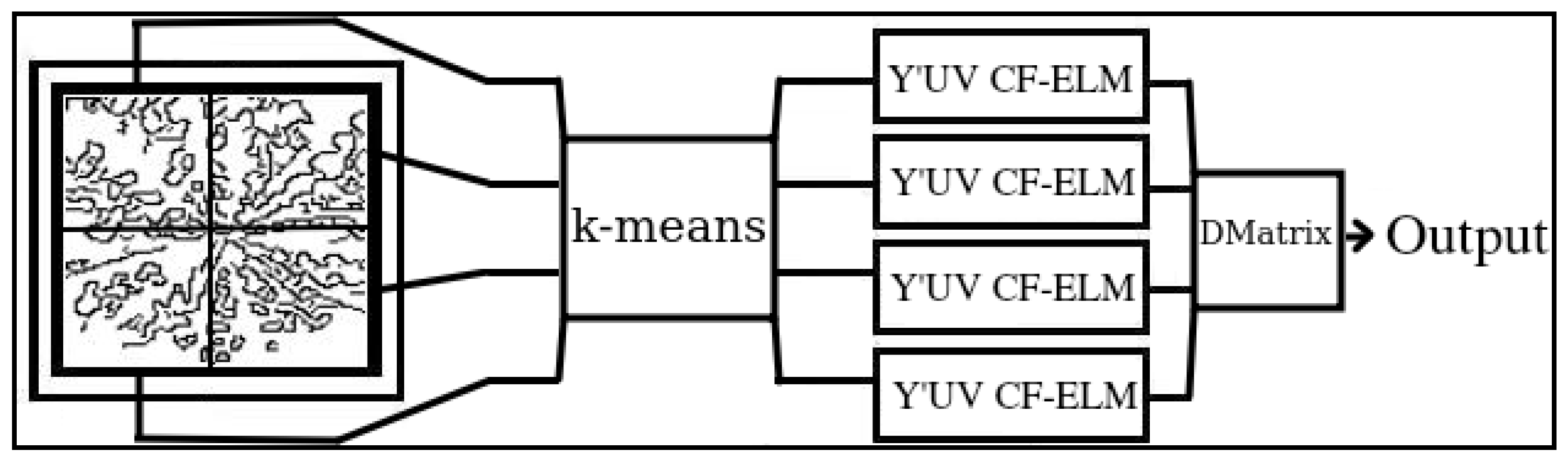
The Colour-feature Extreme Learning Machine (CF-ELM) is a single layer, feed forward neural network based on the Extreme Learning Machine (ELM) [20] with a partially connected, three tier hidden layer and a fully connected output layer. This differs from the ELM which has a fully connected hidden layer. During the training phase the summation of the product of the random weight values and the inputs are stored in the hidden layer output matrix H , to transform the input signal into an output signal the values are first processed through an activation function g ( · ) [21]. The CF-ELM is typically processed with the soft-sign activation function g ( x ) and this can be expressed [22]:
g ( x ) = x 1 + x
The H matrix can be expressed [12]:
H ( W 1 , W N ˜ , b 1 , b N ˜ , Y 1 , Y N , U 1 , U N , V 1 , V N ) = g ( W 1 · Y 1 + b 1 ) g ( W N ˜ · Y 1 + b n ˜ ) g ( W 1 · Y N + b 1 ) g ( W N ˜ · Y N + b n ˜ ) g ( W 1 · U 1 + b 1 ) g ( W N ˜ · U 1 + b n ˜ ) g ( W 1 · U N + b 1 ) g ( W N ˜ · U N + b n ˜ ) g ( W 1 · V 1 + b 1 ) g ( W N ˜ · V 1 + b n ˜ ) g ( W 1 · V N + b 1 ) g ( W N ˜ · V N + b n ˜ ) 3 N · N ˜
where H is the hidden layer output matrix, N is the number of samples used in the training phase and N ˜ is the number of neurons in the hidden layer. In the activation function g ( · ) , W is the input weight and b is the bias. Here the colour input sample values are expressed as Y , U and V for each pixel value. This differs from the ELM which only uses grey-scale values, but has an identical output layer.
The hidden layer output then becomes the input multiplier for the output weights β . The output target T of the CF-ELM is then the result of β · H .
T = β · H
Here β can be expressed:
β = β 1 T β N ˜ T N ˜ · m
where m is the number of neurons in the output layer, which is equivalent to the number of outputs of the ANN. The matrix of target outputs T can be expressed as:
T = t 1 T t N T N · m
where for each t the value is stored based on the input training sample and its desired output (typically a vector of 1 s). This leaves β as the one unknown, by making β the subject we get:
β = H 1 · T
where H 1 is the Moore-Penrose pseudo inverse [23] of matrix H . The output values of this process are then stored in β and used as the weights in the output layer removing the need for a long gradient descent based training process. The classification function is a feed forward summation of the dot product between the input image and the weights in the hidden layer and a dot product with the output layer. The hidden layer is split into 3 for each colour attribute, therefore the number of hidden layer neurons needs to be divisible by 3. For Y’UV, the classifier function for output y i of m classes can be expressed:
y i = j = 1 N ˜ 3 ( β i j ( W j · Y + b j ) + β i j + N ˜ ( W j + N ˜ · U + b j + N ˜ ) + β i j + 2 N ˜ ( W j + 2 N ˜ · V + b j + 2 N ˜ ) )
where W j is the weight vector for the j t h neuron, matched to the beta weight value for the output layer and Y , U and V are the pixel vectors for each colour attribute for a single image. The base of this function, while removing β , was used to generate the H matrix.

2.2. Equal K-Means

The K-means clustering algorithm is an unsupervised learning technique that can be used to split collections of data items into individual clusters [24]. Each cluster is represented by a centroid depicting the mean of the collection of items within a cluster. Typically the algorithm will start by randomly choosing a data item as the initial centroid. Each data item is tested against the centroid to obtain a distance. Successive iterations of the algorithm will test each data item against the centroid made from the mean of the closest matching items. If no changes are recorded during an iteration, the algorithm is said to have converged and ends. The most common distance function is the Euclidean distance function, this can be expressed [25]:
d = ( x 1 y 1 ) 2 + ( x 2 y 2 ) 2 + ( x n y n ) 2
where (x, y) are the centroid and an individual data item, n is the number of data points that make up each data item. Improved K-means algorithms typically utilise a method to select the initial cluster centroids [26]. This improves the speed of convergence, which was not necessary for an image where initial clusters can be based on the location of features. Equal K-means is a variation of the K-means algorithm that dictates that each cluster should be of an equal size [27]. This implementation is useful in image processing where individual segments (or features) of an image need to be clustered and each segment needs to be utilised based on its cluster. For Neural Networks this means that all clusters will be utilised in a predetermined subsection of the network or in the case of this research, an independent classifier. This research utilises Equal K-means and proposes the following algorithm for fast selection of individual clusters.
Algorithm 1 is used in both determining the clusters in training and in detection, utilising the centroids determined in training. Here μ 1 μ k is equal to the centroids for each cluster, where k is the number of centroids and number of image segments, S is each image segment, C is an array where each value has been initialised to zero and this stores the cluster number for the image segment. Where min is set to the max float value for each iteration of S. For each iteration of μ the image segments are checked to find the image segment of closest distance. Once the closest image segment is found, the image segment is not checked against the successive centroids C.
Algorithm 1 Equal K-means
Require: μ 1 μ k
Require: S 1 S k
  1:
functionkmeans
  2:
    k l e n g t h ( μ )
  3:
     C ( 0 1 0 k )
  4:
    for  i 1 to k do
  5:
         m i n m a x
  6:
         m i n _ i n d e x ← 0
  7:
        for  j 1 to k do
  8:
           if  C j ! = 0 then
  9:
                c o n t i n u e
10:
           end if
11:
            d i s t a n c e d ( μ i , S j )
12:
           if  d i s t a n c e < m i n  then
13:
                m i n d i s t a n c e
14:
                m i n _ i n d e x j
15:
           end if
16:
        end for
17:
         C m i n _ i n d e x i
18:
    end for
19:
    return C
20:
end function
The image in Figure 1 depicts the mapping of features between two low resolution images of cows. This was processed using Algorithm 1 at pixel block level. In this example sub image A is being recreated uisng a block of pixels from sub image B and stored as sub image C. Each block of pixels represents a feature within each image and is being rearranged in the shape of another cow.

2.3. Decision Matrix

A decision matrix is a set of values that can be used in a majority voting system of an ensemble learner to prioritise a list of options [28]. In image processing it can be used to give a higher weight to certain areas or features of an image. In an ensemble classifier this can be used to give greater weight to a classifier results based on the section of the image it is working from. In this study, the decision matrix was designed to give greater weight to the segments in the centre of the image. This helped to alleviate the problem of non-target objects appearing in cropped images and in this case, prioritised features appearing in the centre of the cropped image. The decision matrix can be calculated according to Algorithm 2.
Algorithm 2 Decision Matrix - Square Matrix: First pass
Require: w i d t h k
Require: h e i g h t k
  1:
functiondecision_matrix
  2:
     d [ 0 1 , 1 0 w i d t h , h e i g h t ]
  3:
     m i d N / 2
  4:
    k← 0
  5:
    for  i 1 to w i d t h  do
  6:
        if i > m i d then k k 1
  7:
        else  k k + 1
  8:
        end if
  9:
        l← 0
10:
        for  j 1 to h e i g h t  do
11:
            d i , j k + l
12:
           if j > m i d then l l 1
13:
           else  l l + 1
14:
           end if
15:
        end for
16:
    end for
17:
    return d
18:
end function
Algorithm 2 depicts the first pass of calculating the decision matrix (assuming a square matrix), in the second pass the loops and conditions can be reversed to accommodate a matrix, where width and height are calculated based on the number of clusters and are equal to the width and height of the image segments arranged to their location in the image. The final step is to divide by the max value in the matrix to get a weight value. For this research, the decision matrix was used as an optimisation technique.

2.4. Hardware/Implementation Specifics

All algorithms used in benchmarking were programmed in the C programming language and tested on a Manjaro Linux based system, with an i7 processor, 16 gigabytes of RAM and a solid state drive (SSD). The C language was chosen for functionality, portability, efficiency and speed. The pseudo inverse of the matrix H was calculated with assistance from the lapack and lapacke linear algebra libraries [29]. The SCF-ELM was benchmarked against algorithms in a similar class, these included, the Ensemble Extreme Learning Machine (EN-ELM), CIW-ELM, ELM, the C-Support Vector Machine (C-SVC) and linear support vector machine (LSVM) The C-SVC and LSVM were implemented using the libsvm library [18] programmed in C and C++. The EN-ELM was programmed based on Lui and Wang [30] with the discrete cosine transform (DCT) for attribute reduction programmed based on Rod et al. [17]. The EN-ELM was the only algorithm that required preprocessing of the image and for this reason the DCT was included in the bench marking times. In this research the DCT was optimizing by merging the main function with the normalization section and reducing the number of iterations to the desired 81 attributes. The coefficients and cosine values were processed prior to implementation. This provided a fast implementation of the DCT. The ELM was the standard algorithm [18] and was the base used in the EN-ELM, CF-ELM and SCF-ELM. The recording of training and test times were conducted using the c l o c k _ g e t t i m e function which was imported from the t i m e . h library in the c programming environment and the C L O C K _ M O N O T O N I C option was used, as it delivered more accurate times for parallel processing. All images were pre-cropped and scaled to 100 by 100 pixels matching the 10,000 total weights in the input layer of the CF-ELM, this resolution was chosen as a compromise between high resolution accuracy and faster processing speeds. All images were stored as JPEG (4:4:4 sampling) in 100 by 100 pixel dimension and retrieved using the libjpeg library, JPEG was chosen, as it is the default output file type for a number of low resolution cameras used in remote interfaces, it was also the best option considering remote storage and file transfer restrictions. The Y’UV colour space was used in the implementation of the CF-ELM and SCF-ELM. To convert to Y’UV the formula ITU-R B.601 defined by the International Telecommunications Union was adopted [31,32].

2.5. Training/Testing Algorithms

The training algorithm differed from [12], the Sobol sequence [33] was used to generate quasi random weights for the hidden layer of the CF-ELM, providing a uniform distribution of weight values. The same hidden layer was used for all CF-ELMs generated in the ensemble, where the number of CF-ELMs matches the number of image segments, this means that a CF-ELM was trained for each segment as depicted in Algorithm 3.
Algorithm 3 SCF-ELM Training
Require: I m a g e s 1 I m a g e s N
  1:
S [ I m a g e s 11 , , I m a g e s N k ]
  2:
C ← ( 1 , , k )
  3:
W [ w 11 , , w N ˜ P ]
  4:
B ( b i , , b N ˜ )
  5:
functionTrain(S[][],W[][],B[])
  6:
    for  i 1 to k do
  7:
         β i H [ W · S C i + B ] i 1 · T
  8:
    end for
  9:
    return  β
10:
end function
Where N is the number of training images, P is the number of pixels per image, N ˜ is the number of neurons in the hidden layer and k is the number of clusters. Each image segment S had Y , Cr and Cb vectors, this is expounded in Equation (2) of the H matrix. Here C is initialised with Algorithm 1. The number of hidden layer neurons was set to P , where P is the number of inputs [34]. This was found to be an optimal amount of neurons in pretesting. Given the size of the ensemble, this was a necessary trade off between accuracy and performance, avoiding the necessity of a large number of hidden layer neurons.
Testing utilises a majority voting system, the algorithm is made up of four sections, in the first instance the image is divided into image segments, the individual image segments are then matched to the individual cluster centroids determined in training. The decision matrix is added each time a result is within a threshold. This is depicted as a block diagram in Figure 2 and in Algorithm 4. Where a threshold θ is a float distance to the target T set in training. The results in this paper utilised a two class system, each CF-ELM was trained twice, once for the target object and once for images of the surrounding landscape. For a two class system, instead of θ , the decision threshold would be I f ( | T i o u t p u t 1 | < | T i o u t p u t 2 | ) . The a threshold Θ is set to half the max of the sum of the weight values in the decision matrix. This can be adjusted higher or lower for fine tuning accuracy. The decision function in Algorithm 4 is expounded in Equation (7).
Algorithm 4 SCF-ELM Testing - for the i t h image
Require: I m a g e i
Require: β train()
Require: Ddecision_matrix()
  1:
S [ I m a g e i 1 , , I m a g e i k ]
  2:
Ckmeans()
  3:
W [ w 11 , , w N ˜ P ]
  4:
B ( b i , , b N ˜ )
  5:
functionPredict(S[][],W[][],B[],C[])
  6:
     p 0
  7:
    for  j 1 to k do
  8:
         o u t p u t i β j · [ W · S C j + B ] j
  9:
        if  | T i o u t p u t j | < θ  then
10:
            p p + D C j
11:
        end if
12:
    end for
13:
    if  p > Θ  then
14:
        return  T r u e
15:
    end if
16:
    return  F a l s e
17:
end function

2.6. Benchmarking Details

RGB was the default colour system when decoding from JPEG. For this reason, the algorithm differed slightly for each CF-ELM, each took an RGB input that was converted to different colour systems in the case of YCrCb. All algorithms including the EN-ELM, CF-ELM, CIW-ELM, ELM and C-SVC were trained as two class systems, with a positive class of the target object and a negative class of the surrounding landscape. In the case of the ELM implementations the output that was the lowest (or closest to one) was considered the identified class. The SCF-ELM was trained with 99 neurons so that the number of neurons was divisible by 3. The weights and biases in the hidden layer were generated from quasi random numbers from the Sobol sequence. All other ELMs were trained using 100 neurons with pseudo random weights set between 0 and 1 and the biases in the hidden layers set between 0 and 0.1. The weights and biases that worked best differed between each dataset and method. The values for each colour system and DCT were normalised to between 0 and 1. The softsign activation function [35] was used in all of the ELM implementations. These values were selected based on pre-testing and delivered the most consistent results for each of the classifiers.

2.7. Data Sets

The datasets examined three different agricultural robotic applications: (i, ii) Weed, (iii) ATV and (iv) cattle detection, all images were stored as 100 by 100 resolution and pre cropped to border the associated object. An aspect ratio of 1:1 was chosen as a consistent number of pixel inputs were required. A square image provided the best coverage in the case of these datasets. The resolution was based on pretesting as a compromised between processing speed and accuracy metrics. The amount of images in each dataset are available in Table 1. The datasets were split for 10-fold cross validation, 10% for testing and 90% for training.
Specifications of each dataset are as follows:
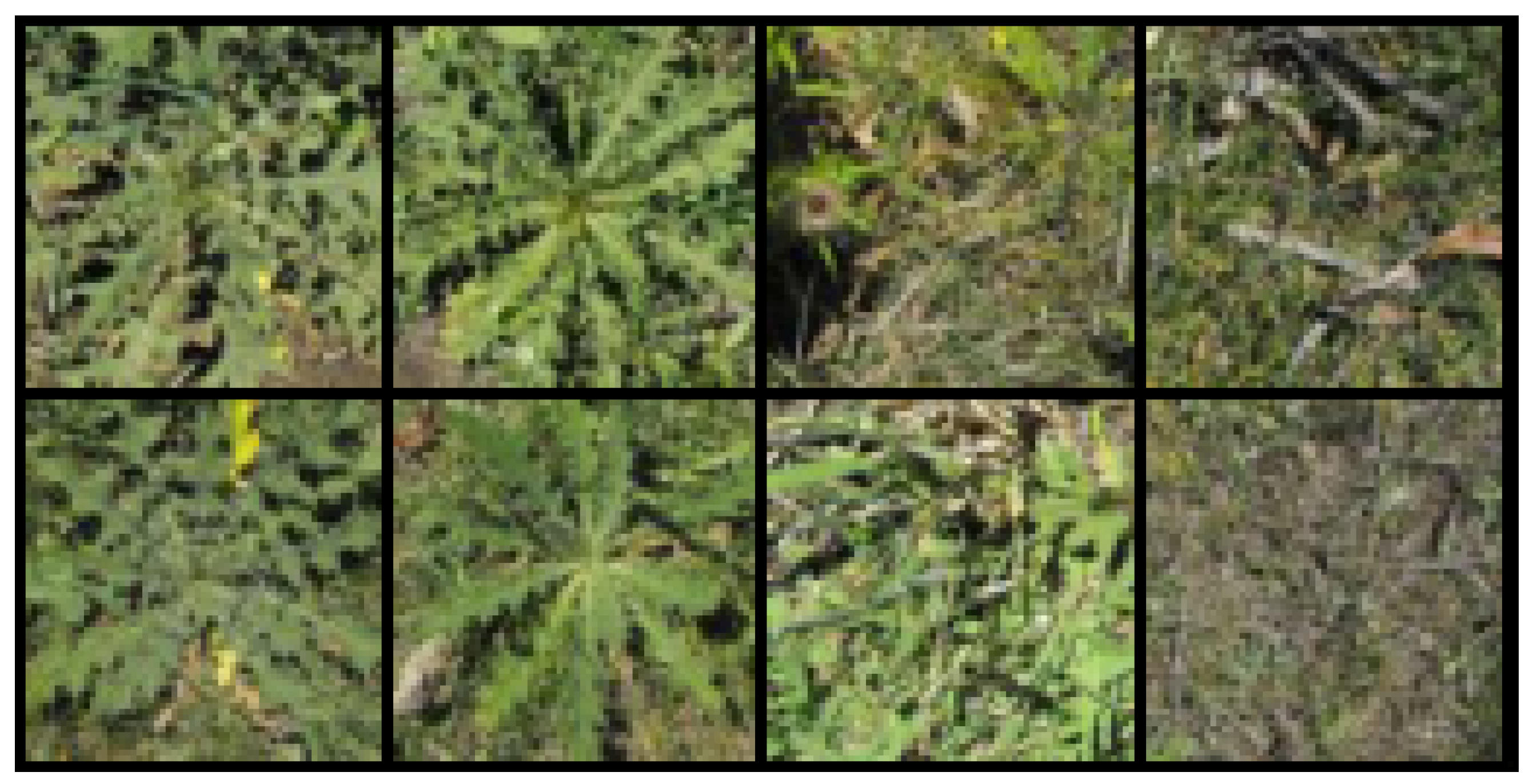
  • Bull Thistle: The Cirsium Vulgare (or Bull Thistle) and surrounding landscape were cropped to eliminate background. These images were photograph using a Fujifilm 10 megapixel hand held camera, at a fixed distance of 2m and nadir geometry. Bull thistle can cause injury to livestock and competes with pasture growing in the area, this has become a problem in eastern areas of Australia [36]. Samples from this dataset are on display in Figure 3.
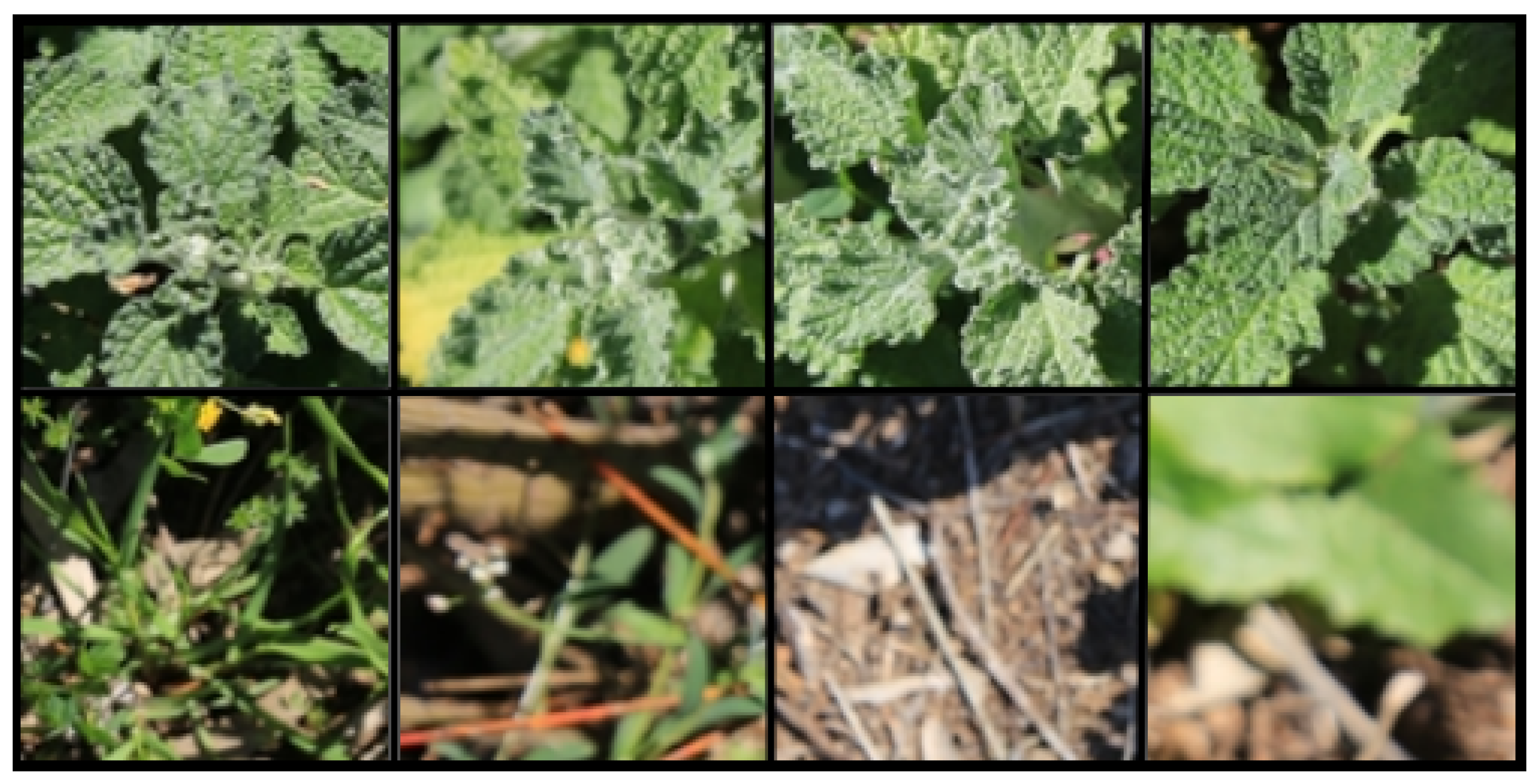
  • Horehound: The Marrubium vulgare (or Horehound) and surrounding landscape were cropped to eliminate background. These images were photograph using a Cannon EOS 6D 20 megapixel hand held camera, at a fixed distance of 2m and nadir geometry. Horehound is unpalatable for livestock and competes with pasture growing in the area, this weed has also become a problem in eastern areas of Australia [36]. Samples from this dataset are on display in Figure 4.
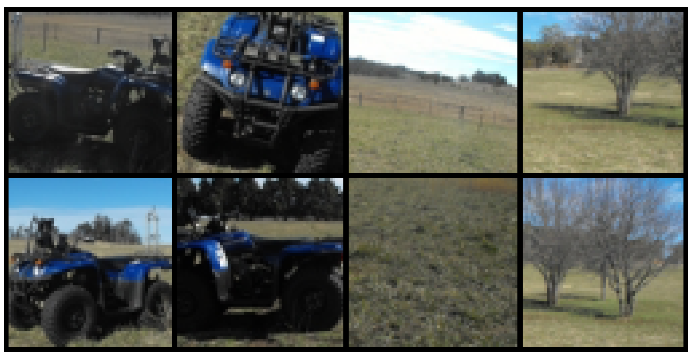
  • Vehicle detection: The vehicle detection dataset contains cropped images of an all terrain vehicle (ATV) on farm land and surrounding landscape. The ATV was photographed using a Fujifilm 10 megapixel hand held camera at a fixed distance of 5 m and at oblique angles and random orientations to simulate a drone fly over. ATV accidents are a major cause of injury and/or death in farm related incidents [37]. A collection of samples from the dataset are available in Figure 5.
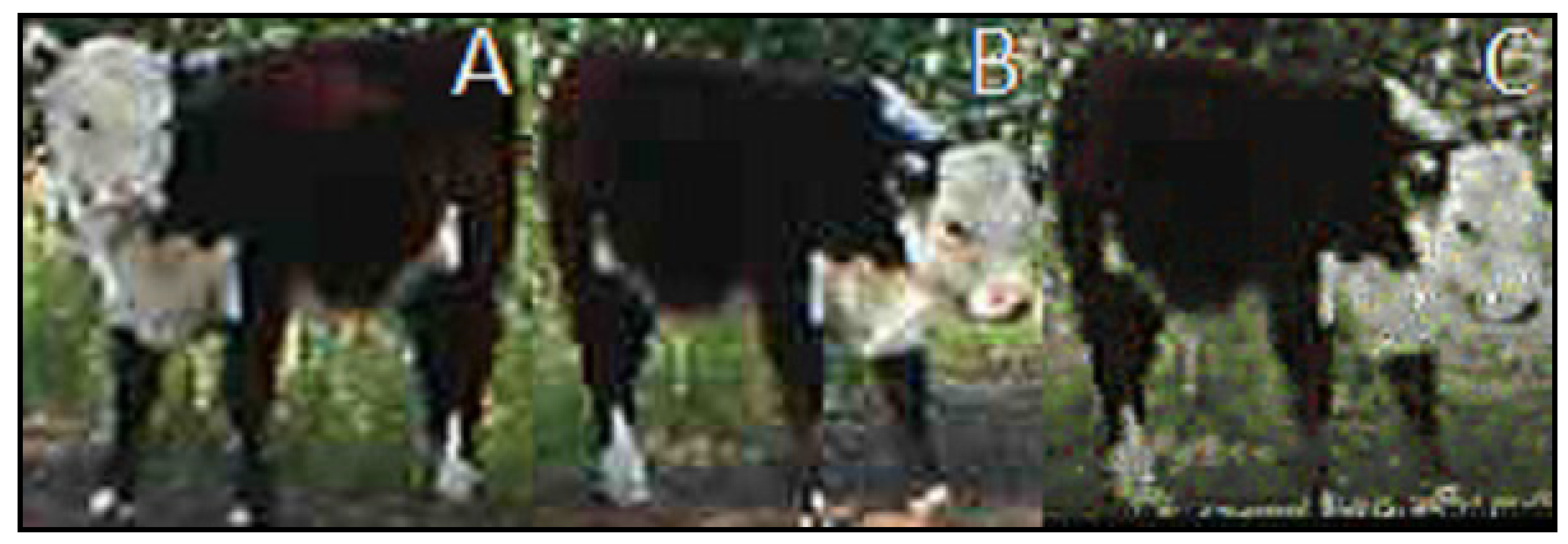
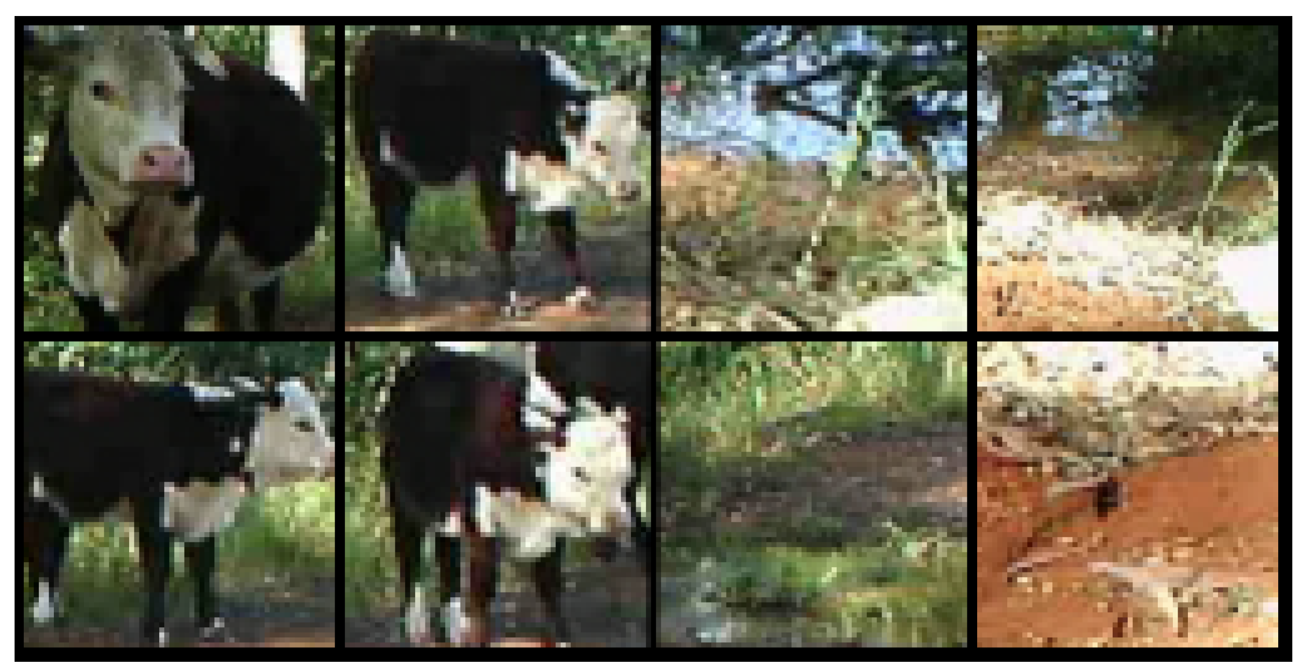
  • Cattle detection: The cattle detection dataset contains cropped images of Poll Herefords in and of a farming landscape. The images were cropped from multiple stationary surveillance cameras that were position at different creek beds waiting for animals to come to drink. These images were captured in AVI video format using a Scoutguard SG860C camera with 640 by 480 pixels at 16 frames per second for 1 min. Image frames were extracted into JPEG format at 1 frame per second, cropped to surround the cattle. The purpose of this dataset is determine if the algorithms could be used in the tracking and counting of cattle. A sample of the image set is displayed in Figure 6.

3. Results

The results include train and test times, true positive rates (TPR), false positive rates (FPR) and accuracy metrics evaluated across all agricultural datasets.

3.1. Dataset Test Results

The datasets used in this section included weed detection (Bull Thistle and Horehound), live stock detection (cattle) and vehicle detection (ATV). The datasets were tested on the proposed SCF-ELM and for comparison were tested against the linear Support Vector Machine (LSVM), the C-Support Vector Classification algorithm (C-SVC), the ensemble ELM (EN-ELM), the Colour-feature Extreme Learning Machine (CF-ELM), the explicit computation of input weights ELM (CIW-ELM) and the standard Extreme Learning Machine (ELM).
Metrics were recorded in three tables for each of the datasets and included: Training time, testing time per image, True Positive Rate (TPR), False Positive Rate (FPR), Precision and classification accuracy (ACC). Recall was not included, as TPR is identical to recall. The results in were recorded using 10-fold cross validation. The number of ensembles for the EN-ELM was based on the algorithm in literature [30], while the number of classifiers in the SCF-ELM was preset at 225, one for each image segement. The C-SVC training time included a grid search to find optimum C and gamma values. This was a requirement to get the best results from the classifier. All times were in seconds, TPR is the percentage of correct classifications against the total, FPR is the percentage of incorrect classifications against the total, precision and accuracy can be expressed:
A C C = T P + T N T P + F P + T N + F N
P r e c i s i o n = T P T P + F P
where TP is true positives, FP is false positives, TN is true negatives and FN is false negatives.
Table 2, Table 3, Table 4 and Table 5 contain the results for testing with each of the datasets; the SCF-ELM and EN-ELM were both ensemble learners that required a longer training phase to collaborate. This was decided based on a tradeoff between accuracy and processing time. The C-SVC required a grid search to get optimum C and gamma values, this was conducted using the grid.py script available in the libsvm package and the time function in the bash console. This is reflected in the results with the C-SVC displaying the slowest training time, followed by the EN-ELM and SCF-ELM. The ELM was the fastest in training followed closely by the CF-ELM. The ELM was also the fastest in testing time per image, while the SCF-ELM provided the highest accuracy in all four datasets. The SCF-ELM was slower in inference times as compared to the other (non-ensemble) classifiers. This was due in part to the feature mapping algorithm, but k-means still managed to converge after just two iterations using the proposed Algorithm 1. The ATV was easier to separate from the surrounding landscapes and the highly optimised linear SVM was able to generalise the solution quite quickly. Producing the fastest training and testing times. For convenience the best results have been underlined in Table 2, Table 3, Table 4 and Table 5.

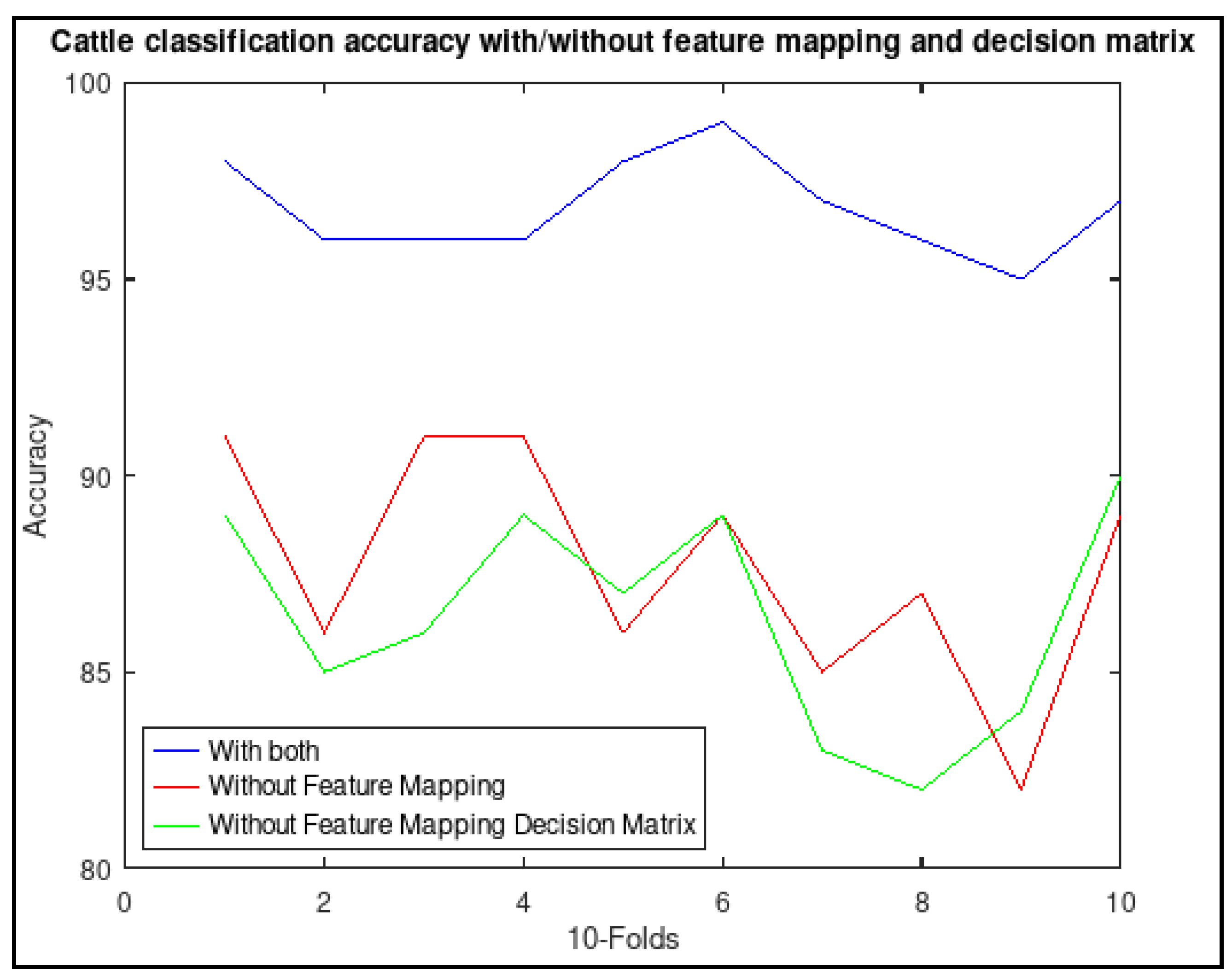
3.2. Benefits of Feature Mapping and Decision Matrix

To demonstrate the benefit of matching individual image segments (or features) to individual CF-ELMS, Figure 7 has three tests based on 10 fold cross validation and the cattle dataset. In the first case (blue), the SCF-ELM was trained with feature mapping and decision matrix, in the second case (red), the SCF-ELM without feature mapping and in the third case (green), the SCF-ELM without decision matrix and feature mapping. It can be seen that feature mapping improves the accuracy by almost 10 percent. Removing the decision matrix has some effect, decreasing the average accuracy over the 10 folds.

4. Discussion

Remote object detection applications often require results in real time and and as a result less computationally intensive algorithms are typically utilised [38]. The performance can be adequate, but may suffer from differing levels of consistency or accuracy e.g., randomizing of weights in the case of an ELM.
It is worth noting that the SCF-ELM did not have the level of optimisation of the libsvm package. This is due in part to the libsvm’s long development cycle [18]. However, the processing times are still comparable and the results in each case were still superior to the C-SVC with radial basis function. The SVM also still suffers from the proliferation of support vectors [6], while a shallow network such as the ELM utilises a consistently sized framework. Given these points, it is a good indication of the SCF-ELM suitability in this space. It is worth noting that the ELM does have further performance optimisation available in literature [19] and this may improve the detection accuracy of the base model ELM and hence the SCF-ELM that uses compatible architecture. Improvements could also be made to both the majority voting and decision matrix algorithms. The decision matrix could be improved by formulating the weighting based on the distance to the chosen centroid for example, but this may increase processing times. The emphasis in this research however, has been on minimal pre-processing and therefore less computational intensive approaches. As this may be a necessity in remote environments, where rapid retraining to new environments is desirable.
The testing times for both implementations also appear adequate for use in a real-time object detection scenario and it is proposed that this research could be used in a remote computer based application. Unmanned aerial vehicles (UAVs) or alternatively unmanned ground vehicles (UGVs) for example can deliver real-time video footage for processing to a remote computer (for convenience a mobile tablet or laptop) via wireless connection [39]. Image frames from video footage can then be extracted for processing purposes and be classified quickly for real-time results. From these results, attached robotics can administer chemicals in the case of weed detection, count or track cattle or return location data in the case of vehicle detection. Due to the ELMs smaller framework and consistent network structure, the ELM is better suited than many of the deep learning and stastical approaches to object classification utilised in remote computing. It is desirable that an algorithm be memory efficient, be able to process images quickly and with a high level of accuracy. The hypothesis stated that the ELM would be well suited as an ensemble learner and the results depicted in this research confer this reality.
It is worth noting that the field of machine learning is a fast moving field and there may exist new implementations of the ELM and other neural based methods that could improve upon the results depicted in this research. This paper placed emphasis on using the standard ELM as many ELM implementations add processing time to the training and testing stages [40]. The CIW-ELM was included in the results to demonstrate the significance of the CF-ELM on these datasets. It also adds little to the training time while demonstrating an improvement in detection consistency in two of the three datasets. The EN-ELM was included as it is a well known ensemble learner in the ELM space. The LIBSVM has been included as it is a leading algorithm that doesn’t have the processing constraints of methods such as the convolutional neural networks (CNN). CNNs have a preference for deep structures [16] and this will impact directly with storage processing requirements in a battery operated device.
In summary, the results depict the SCF-ELM’s ability to improve upon the results of the CF-ELM and with feature mapping, function better on objects with uniform features and with performance metrics comparable or better than some state-of-the-art algorithms.

5. Conclusions

A feature mapping ensemble (or segmented) colour extreme learning machine (SCF-ELM), has been compared to other algorithms in its class, including the LSVM, C-SVC, EN-ELM, CF-ELM and ELM. The classifiers were tested on four datasets, including a weed detection dataset containing bull thistle and surrounding landscape in a paddock. Another weed detection dataset containing Horehound and surrounding landscape in a paddock. ATV detection dataset, where an ATV was positioned in different areas of a paddock and images taken at multiple angles and a cattle detection dataset taken from surveillance footage from a near by farm. The results showed that the SCF-ELM performed comparable or better in each of the four datasets. Future research will involve using the SCF-ELM as a low resolution feature extraction and object detection algorithm, testing a range of custom colour spaces and incorporating feature mapping into a single colour feature based classifier.

Author Contributions

Conceptualization, E.J.S. and G.F.; methodology, E.J.S.; software, E.J.S.; validation, E.J.S.; formal analysis, E.J.S.; investigation, E.J.S.; resources, E.J.S., G.F., D.M. and D.W.L.; data curation, E.J.S.; writing—original draft preparation, E.J.S.; writing—review and editing, G.F.; visualization, E.J.S.; supervision, G.F., D.M. and D.W.L.; project administration, E.J.S.; funding acquisition, D.M. All authors have read and agreed to the published version of the manuscript.

Funding

This research was supported in part by a Cooperative Research Centres Project (CRC-P) Grant from the Australian Government. E. Sadgrove was supported by an Australian Government Research Training Program (RTP) stipend.

Institutional Review Board Statement

Animal Ethics UNE AEC12-042, collected under scientific licence Sci Lic SL 100634.

Data Availability Statement

The data used in this study can be made available by request.

Acknowledgments

Paul Meek, NSW Department of Primary Industries for the provision of cattle surveillance data. Animal Ethics UNE AEC12-042, collected under scientific licence Sci Lic SL 100634. Paul Arnott, UNE Kirby Smart Farm, for access to paddocks for photography of weeds and the ATV. Agent Oriented Software (AOS) and Department of Primary Industries (DPI) for providing the Horehound weed dataset. One of us (D.W.L) would like to acknowledge the support of Food Agility CRC Ltd, funded under the Commonwealth Government CRC Program. The CRC Program supports industry-led collaborations between industry, researchers and the community.

Conflicts of Interest

The authors declare no conflict of interest.

Abbreviations

The following abbreviations are used in this manuscript:
ACCAccuracy
ANNArtificial Neural Network
ATVAll Terrain Vehicle
CF-ELMColour Feature Extreme Learning Machine
CNNConvolutional Neural Network
CIW-ELMComputed Input Weights Extreme Learning Machine
C-SVCC-Support Vector Machine
DCTDiscrete Cosine Transform
ELMExtreme Learning Machine
EN-ELMEnsemble Extreme Learning Machine
LSVMLinear Support Vector Machine
MEC-ELMMultiple Expert Colour Feature Extreme Learning Machine
SCF-ELMSegemented Colour Feature Extreme Learning Machine
SVMSupport Vector Machine
TPRTrue Positive Rate
FPRFalse Positive Rate
YCrCbLight intensity, chrominance red and blue.
Y’UVLight intensity, chrominance red and blue.

References

  1. Gonzalez-Gonzalez, M.G.; Blasco, J.; Cubero, S.; Chueca, P. Automated Detection of Tetranychus urticae Koch in Citrus Leaves Based on Colour and VIS/NIR Hyperspectral Imaging. Agronomy 2021, 11, 1002. [Google Scholar] [CrossRef]
  2. Rahman, M.; Robson, A.; Salgadoe, S.; Walsh, K.; Bristow, M. Exploring the Potential of High Resolution Satellite Imagery for Yield Prediction of Avocado and Mango Crops. Proceedings 2019, 36, 154. [Google Scholar] [CrossRef] [Green Version]
  3. Daga, A.P.; Garibaldi, L. GA-Adaptive Template Matching for Offline Shape Motion Tracking Based on Edge Detection: IAS Estimation from the SURVISHNO 2019 Challenge Video for Machine Diagnostics Purposes. Algorithms 2020, 13, 33. [Google Scholar] [CrossRef] [Green Version]
  4. Palumbo, M.; Pace, B.; Cefola, M.; Montesano, F.F.; Serio, F.; Colelli, G.; Attolico, G. Self-Configuring CVS to Discriminate Rocket Leaves According to Cultivation Practices and to Correctly Attribute Visual Quality Level. Agronomy 2021, 11, 1353. [Google Scholar] [CrossRef]
  5. Bishop, J.; Falzon, G.; Trotter, M.; Kwan, P.; Meek, P. Livestock Vocalisation Classification in Farm Soundscapes. Comput. Electron. Agric. 2019, 162, 531–542. [Google Scholar] [CrossRef]
  6. Hsu, D.; Muthukumar, V.; Xu, J. On the proliferation of support vectors in high dimensions. arXiv 2020, arXiv:math.ST/2009.10670. [Google Scholar]
  7. Zhang, M.; Luo, H.; Song, W.; Mei, H.; Su, C. Spectral-Spatial Offset Graph Convolutional Networks for Hyperspectral Image Classification. Remote Sens. 2021, 13, 4342. [Google Scholar] [CrossRef]
  8. Chand, A.A.; Prasad, K.A.; Mar, E.; Dakai, S.; Mamun, K.A.; Islam, F.R.; Mehta, U.; Kumar, N.M. Design and Analysis of Photovoltaic Powered Battery-Operated Computer Vision-Based Multi-Purpose Smart Farming Robot. Agronomy 2021, 11, 530. [Google Scholar] [CrossRef]
  9. Huang, G.B.; Zhu, Q.Y.; Siew, C.K. Extreme learning machine: Theory and applications. Neurocomputing 2006, 70, 489–501. [Google Scholar] [CrossRef]
  10. Wang, X.; An, S.; Xu, Y.; Hou, H.; Chen, F.; Yang, Y.; Zhang, S.; Liu, R. A Back Propagation Neural Network Model Optimized by Mind Evolutionary Algorithm for Estimating Cd, Cr, and Pb Concentrations in Soils Using Vis-NIR Diffuse Reflectance Spectroscopy. Appl. Sci. 2020, 10, 51. [Google Scholar] [CrossRef] [Green Version]
  11. Xu, J.; Zhou, H.; Huang, G.B. Extreme Learning Machine based fast object recognition. Int. Conf. Inf. Fusion (FUSION) 2012, 15, 1490–1496. [Google Scholar]
  12. Sadgrove, E.J.; Falzon, G.; Miron, D.; Lamb, D. Fast object detection in pastoral landscapes using a Colour Feature Extreme Learning Machine. Comput. Electron. Agric. 2017, 139, 204–212. [Google Scholar] [CrossRef]
  13. Tapson, J.; de Chazal, P.; van Schaik, A. Explicit Computation of Input Weights in Extreme Learning Machines. In International Conference on Extreme Learning Machines; Algorithms and Theories; Springer: Cham, Switzerland, 2015; Volume 1, pp. 41–49. [Google Scholar]
  14. Sheela, K.G.; Deepa, S.N. Review on Methods to Fix Number of Hidden Neurons in Neural Networks. Math. Probl. Eng. 2013, 6. [Google Scholar] [CrossRef] [Green Version]
  15. Sadgrove, E.J.; Falzon, G.; Miron, D.; Lamb, D. Real-time object detection in agricultural/remote environments using the multiple-expert colour feature extreme learning machine (MEC-ELM). Comput. Ind. 2018, 98, 183–191. [Google Scholar] [CrossRef]
  16. Urban, G.; Geras, K.; Kahou, S.E.; Aslan, O.; Wang, S.; Caruana, R.; Mohamed, A.; Philipose, M.; Richardson, M. Do Deep Convolutional Nets Really Need to be Deep (Or Even Convolutional)? arXiv 2016, arXiv:1603.05691. [Google Scholar]
  17. Rod, Z.P.; Adams, R.; Bolouri, H. Dimensionality Reduction of Face Images Using Discrete Cosine Transforms for Recognition. In Proceedings of the IEEE Conference on Computer Vision and Pattern Recognition, Hilton Head, SC, USA, 15 June 2000. [Google Scholar]
  18. Chang, C.C.; Lin, C.J. LIBSVM: A library for support vector machines. ACM Trans. Intell. Syst. Technol. 2011, 2, 27:1–27:27. [Google Scholar] [CrossRef]
  19. Cambria, E.; Huang, G.B.; Kasun, L.L.C.; Zhou, H.; Vong, C.M.; Lin, J.; Yin, J.; Cai, Z.; Liu, Q.; Li, K.; et al. Extreme Learning Machines [Trends & Controversies]. IEEE Intell. Syst. 2013, 28, 30–59. [Google Scholar]
  20. Ertuğrul, Ö.F.; Kaya, Y. A detailed analysis on extreme learning machine and novel approaches based on ELM. Am. J. Comput. Sci. Eng. 2014, 1, 43–50. [Google Scholar]
  21. da Gomes, G.S.S.; Ludermir, T.B.; Lima, L.M.M.R. Comparison of new activation functions in neural network for forecasting financial time series. Neural Comput. Appl. 2011, 20, 417–439. [Google Scholar] [CrossRef]
  22. Wang, Y.; Li, Y.; Song, Y.; Rong, X. The Influence of the Activation Function in a Convolution Neural Network Model of Facial Expression Recognition. Appl. Sci. 2020, 10, 1897. [Google Scholar] [CrossRef] [Green Version]
  23. Barata, J.C.A.; Hussein, M.S. The Moore–Penrose Pseudoinverse: A Tutorial Review of the Theory. Braz. J. Phys. 2011, 42, 146–165. [Google Scholar] [CrossRef] [Green Version]
  24. Kanungo, T.; Mount, D.; Netanyahu, N.; Piatko, C.; Silverman, R.; Wu, A. An efficient k-means clustering algorithm: Analysis and implementation. IEEE Trans. Pattern Anal. Mach. Intell. 2002, 24, 881–892. [Google Scholar] [CrossRef]
  25. Liberti, L.; Lavor, C.; Maculan, N.; Mucherino, A. Euclidean Distance Geometry and Applications. SIAM Rev. 2012, 56, 3–69. [Google Scholar] [CrossRef]
  26. Wang, J.; Su, X. An improved K-Means clustering algorithm. In Proceedings of the 2011 IEEE 3rd International Conference on Communication Software and Networks, Xi’an, China, 27–29 May 2011; pp. 44–46. [Google Scholar] [CrossRef]
  27. Malinen, M.I.; Fränti, P. Balanced K-Means for Clustering. In Structural, Syntactic, and Statistical Pattern Recognition; Fränti, P., Brown, G., Loog, M., Escolano, F., Pelillo, M., Eds.; Springer: Berlin/Heidelberg, Germany, 2014; pp. 32–41. [Google Scholar]
  28. Hashemi, A.; Dowlatshahi, M.; Nezamabadi-pour, H. Ensemble of feature selection algorithms: A multi-criteria decision-making approach. Int. J. Mach. Learn. Cybern. 2021, 1–21. [Google Scholar] [CrossRef]
  29. Netlib.org. The LAPACKE C Interface to LAPACK. Available online: https://www.netlib.org/lapack/lapacke.html (accessed on 24 May 2019).
  30. Liu, N.; Wang, H. Ensemble Based Extreme Learning Machine. IEEE Signal Process. Lett. 2010, 17, 754–757. [Google Scholar] [CrossRef]
  31. Studio Encoding Parameters of Digital Television for Standard 4:3 and Wide-Screen 16:9 Aspect Ratios; Technical Report; International Telecommunications Union, Electronic Publication: Geneva, Switzerland, 2015.
  32. Al-Tairi, Z.H.; Rahmat, R.W.; Saripan, M.I.; Sulaiman, P.S. Skin Segmentation Using YUV and RGB Colour Spaces. J. Inf. Process. Syst. 2014, 10, 283–299. [Google Scholar] [CrossRef] [Green Version]
  33. Harase, S. Comparison of Sobol’ sequences in financial applications. Monte Carlo Methods Appl. 2019, 25, 61–74. [Google Scholar] [CrossRef]
  34. Kim, Y.; Street, W.N.; Russell, G.J.; Menczer, F. Customer Targeting: A Neural Network Approach Guided by Genetic Algorithms. Manag. Sci. 2005, 51, 264–276. [Google Scholar] [CrossRef] [Green Version]
  35. Glorot, X.; Bengio, Y. Understanding the difficulty of training deep feedforward neural networks. In Proceedings of Machine Learning Research, Proceedings of the Thirteenth International Conference on Artificial Intelligence and Statistics; Teh, Y.W., Titterington, M., Eds.; PMLR: Chia Laguna Resort, Sardinia, Italy, 2010; Volume 9, pp. 249–256. [Google Scholar]
  36. Grace, B.S.; Whalley, R.D.B.; Sheppard, A.W.; Sindel, B.M. Managing Saffron Thistle in pastures with strategic grazing. Rangel. J. 2002, 24, 313–325. [Google Scholar] [CrossRef]
  37. Wood, A.; Duijff, J.W.; Christey, G.R. Quad bike injuries in Waikato, New Zealand: An institutional review from 2007–2011. ANZ J. Surg. 2013, 83, 206–210. [Google Scholar] [CrossRef]
  38. Zhang, L.; Zhang, D. SVM and ELM: Who Wins? Object Recognition with Deep Convolutional Features from ImageNet. In Theory, Algorithms and Applications; ELM; Springer: Berlin/Heidelberg, Germany, 2015; Volume 1, pp. 249–263. [Google Scholar]
  39. Zhou, G.; Li, C.; Cheng, P. Conference: Geoscience and Remote Sensing Symposium, Proceedings of the Unmanned Aerial Vehicle (UAV) Real-time Video Registration for Forest Fire Monitoring; IEEE International: Seoul, Korea, 2005; Volume 3. [Google Scholar]
  40. Huang, G.; Huang, G.B.; Song, S.; You, K. Trends in extreme learning machines: A review. Neural Netw. 2015, 61, 32–48. [Google Scholar] [CrossRef] [PubMed]
Figure 1. Feature mapping: Image (B) is being mapped with image (A) as the centroids to image (C).
Agronomy 11 02290 g001
Figure 2. The SCF-ELM with image split into four sections and pixel values sent to four independent CF-ELMs.
Agronomy 11 02290 g002
Figure 3. Images of thistle rosettes and surrounding landscape.
Agronomy 11 02290 g003
Figure 4. Horehound and surrounding landscape.
Agronomy 11 02290 g004
Figure 5. Images of the ATV and surrounding landscape.
Agronomy 11 02290 g005
Figure 6. Images of cattle on the left and surrounding landscape on the right.
Agronomy 11 02290 g006
Figure 7. Accuracy with and without feature mapping and decision matrix.
Agronomy 11 02290 g007
Table 1. Images in each data set, image amounts in training and testing are based on 10-fold cross validation.
DatasetAll ImagesTrainingTestingResolution
Bull Thistle100045050100,100
Horehound100022525100,100
Cattle100045050100,100
ATV100045050100,100
Table 2. Testing results for Bull Thistle for each classifier.
DatasetClassifierTrain Time(s)Time/Image(s)TPRFPRPrecisionAccuracy
Bull ThistleSCF-ELM9.940.011194.0012.8088.0190.60
LSVM2.910.005768.421.6076.0073.40
C-SVC1939.600.006989.6027.6076.4581.00
EN-ELM64.190.004853.2715.9376.9868.67
CF-ELM1.560.002986.4016.0084.3885.20
CIW-ELM4.510.001971.5254.2456.8758.64
ELM1.080.001980.5855.1159.3962.74
Table 3. Testing results for Cattle for each classifier.
DatasetClassifierTrain Time(s)Time/Image(s)TPRFPRPrecisionAccuracy
CattleSCF-ELM9.920.011095.205.4094.6394.90
LSVM1.510.003688.0011.6088.3588.20
C-SVC1749.160.006490.002.8096.9893.60
EN-ELM63.890.004674.0010.9387.1381.54
CF-ELM1.550.002978.1015.8083.1781.15
CIW-ELM4.430.001980.4030.3272.6275.04
ELM1.080.001976.0528.3172.8773.87
Table 4. Testing results for ATV for each classifier.
DatasetClassifierTrain Time(s)Time/Image(s)TPRFPRPrecisionAccuracy
ATVSCF-ELM9.930.011099.81.0099.0199.40
LSVM0.520.001499.601.2098.7199.20
C-SVC591.270.0048100.004.0096.5198.00
EN-ELM64.340.004786.355.7393.7890.31
CF-ELM1.560.002985.927.8891.6089.02
CIW-ELM4.3998580.001976.883.1696.0586.86
ELM1.090.001981.1613.5685.6883.80
Table 5. Testing results for Horehound for each classifier.
DatasetClassifierTrain Time(s)Time/Image(s)TPRFPRPrecisionAccuracy
HorehoundSCF-ELM9.930.011197.2018.2084.2389.50
LSVM3.130.006168.4021.6076.0073.40
C-SVC2037.520.007389.6027.6076.4581.00
EN-ELM60.260.004866.6753.9055.3056.38
CF-ELM1.560.002990.2725.6977.8582.29
CIW-ELM4.510.001970.9251.7757.8059.57
ELM1.080.001973.0555.3256.9158.87
Publisher’s Note: MDPI stays neutral with regard to jurisdictional claims in published maps and institutional affiliations.

