A Multi-Objective Particle Swarm Optimization for Trajectory Planning of Fruit Picking Manipulator

Abstract

Stable, efficient and lossless fruit picking has always been a difficult problem, perplexing the development of fruit automatic picking technology. In order to effectively solve this technical problem, this paper establishes a multi-objective trajectory model of the manipulator and proposes an improved multi-objective particle swarm optimization algorithm (represented as GMOPSO). The algorithm combines the methods of mutation operator, annealing factor and feedback mechanism to improve the diversity of the population on the basis of meeting the stable motion, avoiding the local optimal solution and accelerating the convergence speed. By adopting the average optimal evaluation method, the robot arm motion trajectory has been testified to constructively fulfill the picking standards of stability, efficiency and lossless. The performance of the algorithm is verified by ZDT1~ZDT3 benchmark functions, and its competitive advantages and disadvantages with other multi-objective evolutionary algorithms are further elaborated. In this paper, the algorithm is simulated and verified by practical experiments with the optimization objectives of time, energy consumption and pulsation. The simulation results show that the solution set of the algorithm is close to the real Pareto frontier. The optimal solution obtained by the average optimal evaluation method is as follows: the time is 34.20 s, the energy consumption is 61.89 °/S2 and the pulsation is 72.18 °/S3. The actual test results show that the trajectory can effectively complete fruit picking, the average picking time is 25.5 s, and the success rate is 96.67%. The experimental results show that the trajectory of the manipulator obtained by GMOPSO algorithm can make the manipulator run smoothly and facilitates efficient, stable and nondestructive picking.

1. Introduction

China has been the world’s largest fruit producer, and its output of fruit varieties has ranked at the top globally. Nonetheless, in the scenario of a complicated orchard environment, the whole process of an intelligent picking operation is still difficult to tackle [1]. The intelligent fruit picking operation is mainly divided into three steps: (1) Locating the target fruit by using the visual system; (2) Automatic path planning combined with target positioning information; (3) Motion planning combined with the planned path and completing picking. In the past few decades, many researchers have concentrated on target positioning and path planning, yet have neglected stable and reliable motion planning, the premise for ensuring the completion of a picking operation. Fruit picking without motion planning will cause instability of speed and acceleration in the picking process, a high picking failure rate and is unable to achieve efficient and stable picking. Therefore, in order to achieve efficient and stable picking, the trajectory planning of the robot needs to be deeply studied on the basis of a collision free path.

Due to the manipulator’s operating space and its own characteristics, the planned joint trajectory is supposed to meet the requirements of smoothness and continuity. During the picking process, the manipulator is expected to complete the picking task with low energy consumption in a short time in order to obtain high work efficiency. Accordingly, after obtaining the executable motion trajectory, the trajectory needs to be further optimized [2,3,4]. The optimization of the motion trajectory is to be realized in three main aspects: time, energy consumption and pulsation. Time optimization means that when the kinematic and dynamic constraints are met, the manipulator completes the specified task in the shortest time to enhance the work efficiency of the system. Energy consumption optimization means that the robot completes the specified task with the lowest energy consumption and prolongs the working time of the robot. Pulsation optimization refers to reducing the changes of acceleration of the robot under the condition of meeting various constraints, thus alleviating the impact on the joints and prolonging the service term of the robot. In addition, by optimizing the trajectory of the manipulator, the accuracy of the trajectory tracking of the impact arm can be reduced.

Researchers have conducted in-depth studies on the trajectory optimization of the manipulator. For the multi-objective optimization problems, such as time, energy consumption and pulsation, the multi-objective optimization method is mainly adopted. The specific optimization algorithms include: the weighting coefficient method, the multi-objective genetic algorithm and the multi-objective particle swarm optimization algorithm, and so forth [5].

Shen Yue used the quintic non-uniform B-spline curve interpolation method to plan the trajectory of the manipulator joint space, combined with the weighting coefficient method and the particle swarm optimization method to obtain the trajectory with a short running time and low pulsation [6]. Honggang Duan et al. [7] proposed a trajectory planning method based on execution time, acceleration and jerk for the glass-handling robot. The minimum objective function is established by the weighting coefficient method, consisting of the weighted sum of the square of the integral of the execution time, the integral of the acceleration, and the integral of the jerk. The obtained trajectory not only makes the robot run smoothly, but also improves the working efficiency of the robot. Xu Haili et al. [8] proposed an optimal time and optimal energy trajectory optimization method for industrial robots. The motion trajectory of the robot is regarded as the connection of key points in the robot space. The key points are fitted and connected by cubic polynomial and iterated by the weighting coefficient method, so as to optimize the overall motion time and energy consumption of the robot [8].

R. Saravanan takes the energy consumption and smoothness of the joint trajectory curve as optimization objectives, and uses a non-dominated sorting genetic algorithm II(NSGA-II) to optimize the trajectory of an industrial robot with load, but only for point-to-point tasks in joint space [9]. Qi Ruolong et al. [10,11] studied the trajectory planning of a space robot, transformed the trajectory planning problem of the space manipulator into a multi-objective optimization problem, resolving it by way of a genetic algorithm, and establishing the evaluation function of the manipulator motion angle, maximum torque, total motion time and other parameters through the weighting coefficient method, and ultimately came up with a collision free trajectory with short motion time. Wang Huifang used a high-order B-spline curve to construct the continuous trajectory of manipulator joint space. Taking short motion time, small pulsation and low energy consumption as the optimization objectives, NSGA-II was used to solve the multi-objective optimization problem of manipulator trajectory, and the Pareto optimal solution set was obtained. It was studied and analyzed on a six degrees of freedom robot and was obtained with good optimization results [12]. Wang et al. interpolated the motion path of a micro motion parallel robot by using a 7th degree B-spline curve, and the motion trajectory obtained was stable and continuous [13].

Traditional optimization methods, such as the weighting coefficient method, mostly adopt different strategies to decompose the multi-objective problem into a single objective problem respectively. Then, a single objective algorithm is adopted to complete the optimization, which depends on prior knowledge and is limited by the shape of the Pareto front. Especially when the multi-objective problem presents complex characteristics such as nonlinearity and high dimension, the traditional methods are inadequate to be employed for a significant optimization effect, and are even unable to attain the optimal solution. The NSGA-II algorithm has complex operation and low efficiency, while the multi-objectives particle swarm optimization (MOPSO) algorithm has stronger searching ability, which is conducive to obtaining the optimal solution in the sense of multi-objectives. It is achieved by the whole solution set population, and multiple non-inferior solutions are searched simultaneously in parallel, leading to fast convergence speed and high efficiency. Its coding method has been proven to be simpler than NSGA-II and has good applicability. The algorithm is simple and easy to implement, with a few parameters to be adjusted, yet no gradient information is required. It is suitable for dealing with various types of objective functions and constraints, particularly in engineering applications [14,15,16].

In summary, due to the complex orchard environment, the ultimate goal of a stable, efficient and nondestructive picking manipulator trajectory has been difficult to achieve. In response to the existing issue, aiming at tackling the above-mentioned problems, this paper thoroughly studies the trajectory optimization of the picking manipulator, and proposes an improved multi-objective optimization algorithm. By introducing non-dominated sorting, crowding distance, feedback mechanism, annealing factor and mutation strategy, the convergence and diversity of the MOPSO algorithm are perfected. The main research contents are as follows: (1) A B-spline curve is used for trajectory planning to obtain a smooth manipulator trajectory; (2) Combined with the idea of multi-objective optimization, multiple performance indexes of the manipulator trajectory are optimized at the same time, and the Pareto frontier of the manipulator trajectory planning is obtained. The average optimal evaluation method is used to select the trajectory planning scheme; (3) The above theoretical analysis is verified by practical experiments to prove the effectiveness of the algorithm. Through the research, the stability, efficiency and nondestructiveness of the picking process are effectively promoted, and it provides a theoretical and practical research basis for intelligent picking under complex orchard conditions.

2. Kinematic Model and Path Planning of the Picking Manipulator

2.1. Kinematic Model of the Picking Manipulator

This paper takes the 6-DOF series manipulator, produced by Guangdong Ruobo Intelligent Co., Ltd., as the research object, whose joints are rotating joints, and the sixth joint is connected with the end effector to grasp the target fruit. In order to accurately describe the pose of the manipulator, the D-H rule is applied to determine the coordinate system position of the connecting rod, as shown in Figure 1.

2.2. Path Planning

Trajectory planning needs to be based on collision free path planning. For the purpose of attaining the collision free path, combined with the basis of previous research [17], this paper uses the optimized rapidly-exploring random tree (RRT) algorithm to generate a path. The optimized RRT algorithm introduces the idea of target gravity into the basic RRT algorithm, increasing the path search speed. It combines the improved methods such as the genetic algorithm and the smoothing method to smooth and optimize the path. By applying this algorithm, a collision free and short distance path can be quickly obtained to provide a path basis for trajectory planning. The path planning flow chart is shown in Figure 2.

3. Trajectory Optimization of Manipulator Based on Multi-Objective Particle Swarm Optimization Algorithm

3.1. B-Spline Parameterization

In order to acquire information about the speed, acceleration and jerk of path points, B-spline curve interpolation is carried out for the path points obtained by the above path planning method. Because the B-spline curve has local support, changing the i-th control vertex Pj of the curve only affects the k curves related to the vertex, and the rest of the curves will not be influenced. In accordance with this principle, the speed, acceleration and jerk among path points can be configured arbitrarily, so that the motion trajectory of the manipulator has stronger adaptability [18,19]. Each path point is connected by a section of the B-spline curve, and each section of the B-spline curve is connected smoothly to ensure that the trajectory smoothness requirements are met.

In this paper, a quintic B-spline curve is used to interpolate the joint path to construct the motion trajectory of the manipulator. To interpolate the path with B-spline function, the control vertices of the B-spline curve need to be determined through the path points. The essence of determining the control vertices is to calculate the vertices of the control polygon according to the path point P. The robot joint path point sequence is expressed as (t_i, P_i) i = 0, 1, 2, …, N. The starting time is t₀ and the ending time is tf. The i-th quintic B-spline curve is shown in Equation (1). In order to construct the motion trajectory of the manipulator, B-spline curve interpolation is carried out for the known n path points, and n − 1 quintic B-spline curves are used to connect, so that the starting point and end point of each B-spline curve coincide with the path points. Since the motion at the initial position and the end position is known, n + 5 control vertices Q₀, Q₁, …, Q_n+4 can be obtained.

$$P_{i,5}={\displaystyle \sum _{j=0}^5{Q}_{i+j}{N}_{j,5}(u)},$$

(1)

where P is the path point, Q is the control vertex of the B-spline curve, and u is the node vector; N_j,5 (u) is a quintic normalized B-spline basis function, which can be recursively obtained by the Deboor–Cox formula.

With reference to the above, the first point and the end point are generally consistent with the first data point and the end data point (that is Q₀ = P₀, Q_n+4 = P_n) when inversely calculating the control vertex. Therefore, the repeatability at both ends of the curve is taken as 6. P_i point corresponds to the node value u_{5 +i}, so the B-spline curve corresponds with the node vector U = [U₀, U₁, …, U_N+10]. The cumulative chord length parameterization method is used to normalize the time node to obtain the node vector value [20].

3.2. Multi-Objective Trajectory Optimization of Manipulator

3.2.1. Constraints and Optimization Objectives of Manipulator Trajectory

In order to improve the picking efficiency, the B-spline curve is used to interpolate the path of the manipulator to obtain a smooth motion trajectory with time parameters. On this basis, the trajectory is further optimized to enable the trajectory to meet the kinematic and dynamic constraints of the manipulator and meet the requirements of different performance indexes in the picking task. Combined with the kinematic characteristics of the manipulator, the picking efficiency, energy consumption and pulsation are defined as objective functions respectively to establish a multi-objective trajectory optimization model [21].

To ensure the normal operation of the manipulator, the trajectory of the manipulator must be within the kinematic and dynamic constraints. The specific contents need to meet the following three points.

(1)

Position constraint: the position constraint is that the trajectory curve must pass through each position point of the given path to ensure that the manipulator will not collide with obstacles during movement;

(2)

Joint limit constraint: the rotation angle range of each joint of the manipulator is certain, and the position curve of the manipulator generated by interpolation cannot exceed the rotation angle range of each joint;

(3)

Speed constraint and acceleration constraint: the speed curve and acceleration curve of the manipulator joint shall not only ensure continuity, but also meet the speed constraint and acceleration constraint of the manipulator. The constraint values are shown in

Table 1. Joint motion range and constraints.

Joint Number	Angle Range/(°)	Angular Speed Constraints/(°/s)	Angular Acceleration Constraints (°/s2)
1	−165~165	156	400
2	−55~145	140	400
3	−165~170	156	400
4	−185~185	270	600
5	−120~120	180	600
6	−350~350	430	600

. Assuming that the maximum speed, maximum acceleration and maximum jerk of joint motion are v_m, a_m and jer_m respectively, the trajectory of each joint shall meet the kinematic constraint Equation (2):

$$\left|v(t)\right|\le v_m,\left|a(t)\right|\le a_m,\left|jerk(t)\right|\le je{r}_m m=1,2,\dots ,6,$$

(2)

where m represents the joint number.

In the light of the characteristics of the convex hull of the B-spline curve, the constraints in Equation (2) can be transformed into the control vertices of the B-spline curve of each joint, only under the following conditions:

$$max\left|Q_{km}^1\right|\le v_m$$

(3)

$$max\left|Q_{km}^2\right|\le a_m$$

(4)

$$max\left|Q_{km}^3\right|\le je{r}_m,$$

(5)

where k represents the k-th control vertex of joint speed, acceleration and the acceleration curve.

On the premise of meeting the above constraints, the motion time, pulsation and energy consumption of the manipulator are optimized to give full play to the performance of the robot.

(1)

Time

In order to improve the operation efficiency of the robot, the operation time of the robot is optimized to minimize the time for the robot to move along the specified trajectory under the condition of meeting various constraints. Definition formula (6):

$$S_1=min\left({\displaystyle \sum _{i=1}^{n-1}\mathsf{\Delta }{t}_i}\right)=min\left[{\displaystyle \sum _{i=1}^{n-1}\left(t_{i+1}-t_i\right)}\right],$$

(6)

where S₁ is the total operation time of the manipulator. The smaller S₁ is, the higher the working efficiency of the manipulator is;

n is the number of path points;

i is the number of path points.

(2)

Energy consumption

The working environment of the picking robot is mostly in the field. Reducing energy consumption can effectively improve the continuous working time of the robot when the robot lacks energy supply. The energy consumption expression is:

$$S_2=min\left[{\displaystyle \sum _{m=1}^M\sqrt{\frac{1}{Ti}{\displaystyle {\int }_0^{Ti}{\left(a_j\left(t\right)\right)}^{2}dt}}}\right],$$

(7)

where S₂ is an index used to measure the energy consumption of the joint. The smaller S₂ is, the less energy will be consumed by the joint; a(t) is the acceleration curve of the joint.

(3)

Pulsation

During the movement of the robot, the sudden change of acceleration will have a great impact on the body of the manipulator, reducing the tracking accuracy and destroy the mechanical structure. Therefore, non-abrupt acceleration is the core requirement of trajectory planning. Optimizing the jerk cure of the robot can reduce the impact, promote the accuracy of the motion trajectory and the target trajectory, and further reduce the contact force among the internal components of the manipulator, thus alleviating the vibration intensity during resonance. The pulsation optimal expression is defined as Equation (8):

$$S_3=min\left[{\displaystyle \sum _{m=1}^M\sqrt{\frac{1}{Ti}{\displaystyle {\int }_0^{Ti}{\left(jer{k}_j\left(t\right)\right)}^{2}dt}}}\right],$$

(8)

where S₃ represents the average joint pulsation. Smaller S₃ equates to a smaller pulsation of the joint trajectory and more stable motion;

M is the number of joints;

T_i is the total time of exercise;

jerk (t) is the pulsation trajectory of the joint.

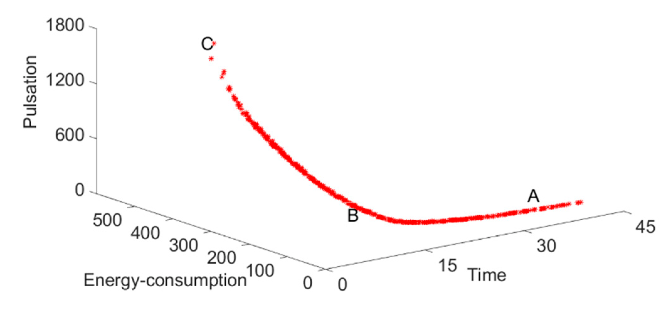
It can be seen from the above that the trajectory of the manipulator needs to meet multiple constraints and needs to be optimized under multiple objectives. Using the multi-objective optimization method, the above multiple objectives can be optimized synchronously to achieve the best overall effect. Due to the conflict of objectives in multi-objective optimization problems, the method to solve multi-objective optimization problems is usually to coordinate and balance among objectives to make each objective optimal as much as possible [22]. The optimal solution is not the global optimal one, but the equilibrium solution of all objectives, the set of non-inferior solutions, called the Pareto optimal solution set, is definitely the chosen one. In order to solve the multi-objective optimization problem of manipulator trajectory, the Pareto optimal solution set is obtained and solved by the multi-objective particle swarm optimization algorithm. The algorithm is an optimization algorithm based on swarm intelligence theory. It depends on cooperation and information sharing among all individuals in the group to find the optimal solution. Individuals will adjust the motion state according to their own experience and group experience, and constantly approach the optimal solution through the evolution of the population [23]. MOPSO uses Pareto optimality and other concepts to evaluate the advantages and disadvantages of particles, and continuously updates the position and speed of particles through individual optimal P_best and global optimal G_best. The update formula is shown in formulas (9) and (10).

$$v_{i+1}=w\times v_i+c_1\times rand\times \left(P_{best}\left(i\right)-x_i\right)+c_2\times rand\times \left(G_{best}\left(i\right)-x_i\right)$$

(9)

$$x_{i+1}=x_i+v_{i+1},$$

(10)

where: v represents the speed of particles;

x represents the position of the particle;

i represents the number of iterations;

w represents inertia weight;

c₁ and c₂ are acceleration factors;

rand is a random number with uniform distribution of [0, 1].

With the aim of better obtaining the individual optimal solution and the global optimal solution, and guiding the algorithm to quickly converge to the Pareto front, this paper introduces the individual violation degree and Pareto constraint domination to evaluate the solution set. In order to strengthen the search ability and convergence speed of the traditional MOPSO algorithm, and shielding if from falling into local optimization, this paper optimizes the MOPSO algorithm by adding a mutation operator, a feedback mechanism and an annealing factor.

3.2.2. Constraints and Pareto Constraints

There are many constraints in multi-objective optimization problems. In order to effectively deal with multiple constraints and to better compare different solutions, an individual violation degree is used to deal with constraints. Individual violation degree is defined as the normalized sum of all conflicting constraint values and it can be described as Equation (11) [24]:

$$violation(x)=\left\{\begin{array}{l}max(0,g_j(x)) \mathrm{if}i=1,2,\dots q\\ \left|h_j(x)\right| \mathrm{if}j=q+1,q+2,\dots ,m\end{array}\right.,$$

(11)

where it is expressed as the distance between solution x and the feasible region. The greater the distance is, the higher the individual violation degree will be. When x is the feasible solution, the individual violation degree is 0.

In the multi-objective optimization algorithm, it is necessary to compare not only the individual violation degree between the two solutions, but also the objective function values. However, the objective function is not unique, so the optimal solution cannot be determined directly. In this paper, the Pareto constraint domination is used to compare the solutions and clarify the relationship between advantages and disadvantages. Solution x_i dominates solution x_j, which must satisfy any of the following conditions:

(1)

If the solutions x_i and x_j are all feasible solutions of the optimization problem, and the solution x_i is Pareto dominated x_j;

(2)

If the solution x_i is feasible and x_j is infeasible;

(3)

If solutions x_i and x_j are infeasible solutions, but solution x_i has less constraint violation degree;

(4)

If both solutions x_i and x_j are infeasible solutions and have the same constraint violation degree, then solution x_i is Pareto dominated x_j.

3.2.3. Mutation Operator

In the MOPSO algorithm, the external file set is devised to store all non-dominated solutions. In each iteration, the global optimal solution needs to be selected from the external file set. In the iterative process of the algorithm, the non-dominated solution will be continuously added to the external file set, resulting in the increasing scale of the external file set, increasing the amount of calculation of the algorithm and reducing the efficiency of the algorithm. Therefore, an upper limit needs to be set on the external file size. When the number of solutions in the external file sets exceeds the upper limit, a certain amount of solutions would be deleted to keep the size of the external file set unchanged. This paper adopts crowding distance sorting to delete the individuals with a small crowding distance and maintain the number of solutions in the external file sets. Crowding distance evaluates the distance between an individual and its adjacent individuals. For an individual in the target space, the distance between the individual and the individuals on both sides is calculated in each target space. The average sum of the distances in each dimension of the target space is the crowding distance. The larger the crowding distance, the sparser the distribution of solution sets, and the better the diversity of solution sets. The crowding distance formula is shown in (12) [25]:

$${\displaystyle \sum _{j=1}^l\frac{\left|f_j\left(x_{i+1}\right)-f_j\left(x_{i-1}\right)\right|}{f_{j\max }-f_{j\min }}},$$

(12)

where f_i(x_i) represents the function value of individual x_i on the j-th objective function;

f_jmax and f_jmin represent the maximum and minimum values of the population on the j-th objective function, respectively.

During optimization, all particle updates rely on the searched non-dominated solutions. The greater the number of non-dominated solutions and the more uniform the distributions are, the better the solution set will be [26,27]. Maintaining the diversity of non-dominated solution sets can avoid premature convergence of the algorithm. Therefore, when maintaining external file sets, mutation operators are added to improve the diversity of solution sets and avoid premature convergence of the algorithm. A mutation operator is added to the external file set to produce a new solution. For each individual in the external archive set, a mutation solution is generated randomly. The generated mutation solution set is compared with the external file set. If an individual in the external file set is dominated by the mutation solution, the mutation solution will replace the dominated individual in the external file set. Otherwise, the mutation solution is discarded. If the random value rand is less than the set probability p, the individual of the external file set is taken as the parent to generate a mutation solution. If the random value rand is greater than the set probability p, no mutation solution is generated. By setting p, the size of the mutation solution set can be controlled, which not only increases the population diversity, but also does not increase the amount of calculation of the algorithm, so as to avoid reducing the efficiency of the algorithm [28]. The mutation solution set can guide particles to fly to a wide area and increase the diversity of solutions in the external file set, so it can reduce the probability of the algorithm falling into local minima. The generation process of the variant solution set is shown in Equation (13):

$$\begin{array}{l}child(x)=p\times paren{t}_1(x)+(1-p)\times paren{t}_2(x)\\ child(v)=\frac{paren{t}_1\left(v\right)+paren{t}_2\left(v\right)}{\left|paren{t}_1\left(v\right)+paren{t}_2\left(v\right)\right|}paren{t}_1(v)\end{array}$$

(13)

where parent(x) represents the position of the parent particle; parent(v) represents the speed of the parent particle; p is the probability of variation.

3.2.4. Feedback Mechanism

In order to ensure the diversity of solution sets in the iterative process, it is necessary to replace the inferior solutions in the solution set. In this paper, the feedback mechanism is used to deal with it: the solution sets after each iteration are arranged in the order of advantages and disadvantages, and a certain number of bad solutions are selected for mutation. For the individuals who have not become optimized after n iterations, individuals are randomly selected from the external solution set to replace them. The solution set is fed back in two ways to improve the diversity of the solution set and to accelerate the convergence speed of the algorithm.

3.2.5. Annealing Factor

In the iterative process of the algorithm, particles are continuously selected from the external file set as the global optimal solution to guide the convergence of the algorithm. Due to the single evolution direction, when a better solution cannot be generated, the population easily falls into local optimization and the real Pareto frontier cannot be found. To solve this problem, an annealing factor is added in the iterative process to accept the poor solution with a certain probability, enhance the diversity of the population and make it jump out of the local optimal solution. The specific process is as follows: when the new solution Q_new dominates the current solution, the new solution Q_new is taken as the individual historical optimal solution. If the new solution does not dominate the current solution, the new solution Q_new is accepted as the individual historical optimal solution with probability P_m, and the expression is shown in Equation (14). It can be seen from the formula that, at the initial stage of the algorithm iteration, there are fewer individuals in the external file set and the P_m value is large. Accepting the poor solution with a large probability can increase the diversity of the population. In the later stage of the algorithm, there are many individuals in the external file set, and a higher P_m value will slow down the convergence speed of the algorithm. To compensate, in the later stage of the algorithm iteration, a small P_m value is adopted [29].

$$P_m=\left\{\begin{array}{l} 1{ \mathrm{Q}}_{new}\prec \mathrm{Q}\\ \frac{t}{T_{\max }}\left(p_{start}-p_{end}\right)+p_{end}{ \mathrm{Q}}_{new}\nprec \mathrm{Q}\end{array}\right.,$$

(14)

where p_start is the initial annealing factor;

p_end is the final annealing factor;

t is the current number of iterations;

T_max is the maximum number of iterations.

The pseudo code of the improved multi-objective particle swarm optimization algorithm (represented as GMOPSO) is shown in the following algorithm. objfun represents the objective function and constfun represents the constraints of the optimization issue:

GMOPSO Algorithm ()

1: Initialize(popsize, archive size, objfun,constfun, iterative times);

2: For each particali ∈ [1, popsize]

3: [xi, vi] ← Initializepositionand speed

4: Initialize individual best solution Pbest

5: end

6: archive ← Determination(pop,objfun,constfun)//sort particals and get non-dominant individuals

7: for it = 1:(iterative times)

8: for each partical

9: Obtain the Gbest

10 :[xi, vi] ← Position_speed(Pbest, Gbest)

11: Pbest ← Update(Pm, Pbest)

12: end

13: pop ← sort (pop, M)//eliminatethe poorerparticals and supplyparticals

14: Update external archive

15: archive ← Mutate(archive, mu)

16: Until stopping criterion is met

17: end

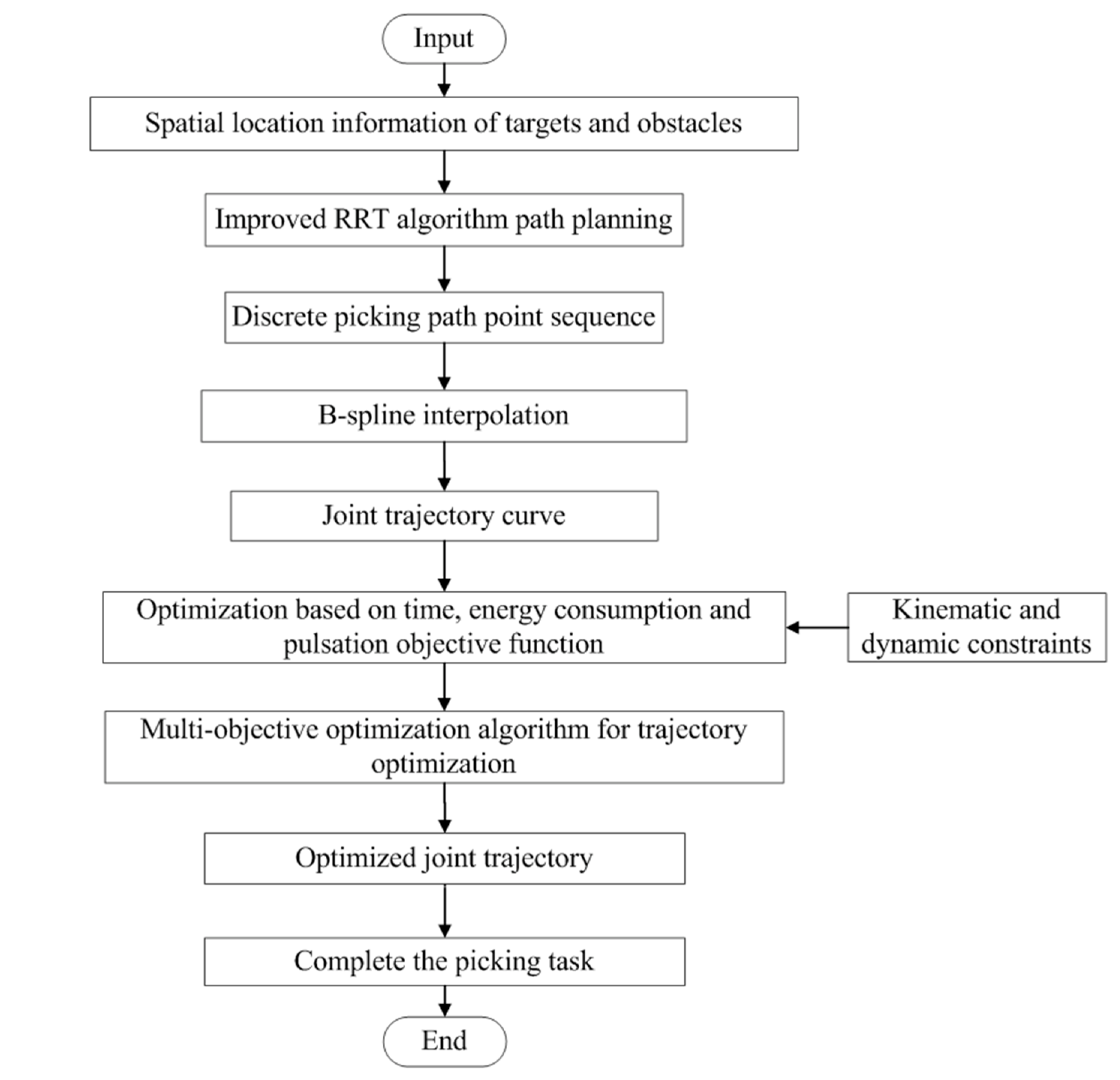
Taking the motion time, energy consumption and pulsation as the optimization objectives, the optimal trajectory optimization model is established. The multi-objective trajectory optimization problem of the manipulator is solved by using the GMOPSO algorithm, so as to obtain the trajectory of the manipulator that meets the constraints and performance requirements. The joint path of the manipulator is interpolated by a quintic B-spline curve to make the manipulator meet kinematic and dynamic constraints. According to the definition of the performance index above, the multi-objective optimization problem with optimal time, energy consumption and pulsation can be defined as Equation (15):

$$\left\{\begin{array}{l}minF(x)=[f_1,f_2,f_3]=[{\displaystyle \sum _{i=1}^{n-1}\mathsf{\Delta }{t}_i,{\displaystyle \sum _{j=1}^6\sqrt{\frac{1}{T}{\displaystyle {\int }_0^{T}jer{k}_i^{2}dt}},{\displaystyle \sum _{j=1}^6\sqrt{\frac{1}{T}{\displaystyle {\int }_0^T{a}_i^{2}dt}}}]}}\\ \left|v_j\right|\le V{M}_j\\ \left|a_j\right|\le A{M}_j\end{array}\right.,$$

(15)

where f₁ is the movement time;

f₂ is the average joint pulsation, which measures the smoothness of the trajectory; and

f₃ is the average joint acceleration. The simplified analysis of the dynamic model of the manipulator shows that the energy consumption of the manipulator is directly proportional to the square of the absolute value of the acceleration. Therefore, the average joint acceleration is defined as the optimization objective as an index to measure the energy consumption of the robot;

VM_j and AM_j represent the maximum speed and acceleration of each joint respectively.

The specific algorithm flow is shown in the Figure 3 below:

4. Test and Analysis

4.1. Performance Verification of GMOPSO Algorithm

In order to verify the effectiveness and accuracy of the GMOPSO algorithm, three classical test functions are selected for the performance test and the simulation test, and are further compared with the basic MOPSO algorithm and the classical multi-objective optimization algorithm NSGA-II. The generational distance (GD), a non-inferior solution spacing measure (represented by SP) and algorithm running time are employed to evaluate. GD, as shown in formula (16), represents the distance between the non-dominated solution set obtained by the algorithm and the real Pareto optimal solution set. The smaller the GD is, the closer the solution set obtained by the algorithm is to the real Pareto front. GD = 0 means that all the solutions obtained by the algorithm are located on the Pareto front, that is, all the solutions obtained are the solutions in the real Pareto optimal solution set. This index reflects the convergence degree between the non-inferior solution set obtained by the algorithm and the real Pareto optimal solution set. The spacing index SP, as shown in formula (17), can be used to measure the distribution of the solution set searched by the algorithm. The smaller the SP value is, the more uniform the solution distribution is. SP = 0 indicates that the front end of the non-inferior solution set obtained by the algorithm is absolutely evenly distributed, and this index reflects the uniformity of the front end of the non-inferior solution set obtained by the algorithm.

$$GD=\sqrt{{\displaystyle \sum _{i=1}^n{d}_i^2/n}}$$

(16)

$$SP=\sqrt{\frac{1}{n-1}{\displaystyle \sum _{i=1}^n{\left(d-d{o}_i\right)}^2}},$$

(17)

where n is the number of non-dominated solutions searched by the algorithm;

d_i is the shortest distance from solution x_i to Pareto front; and

do_i is the distance between the target vector of solution x_i and its nearest target vector;

$$d{o}_i=min\left\{{\displaystyle \sum _{k=1}^l\left|f_k(x_i)-f_k(x_j)\right|}\right\}i,j=1,2,\dots ,n,i\ne j.$$

d is the average value of do_i.

The real Pareto frontier of classical test functions ZDT1, ZDT2 and ZDT3 is known, so it can objectively test the performance of the algorithm. The Pareto front of function ZDT1 is continuous and concave. The Pareto front of function ZDT2 is continuous and nonconvex. The Pareto front of function ZDT3 is discontinuous and convex [30].

Fifty simulation tests are conducted for each test function. The algorithm parameter settings are shown in

Table 2. Parameters of algorithms.

Algorithm	Parameter Settings
	Population Number	Number of External File Sets	Number of Iterations
non-dominated sorting genetic algorithm II(NSGA-II)	300	300	300
multi-objective particle swarm optimization algorithm (MOPSO)	300	300	300
improved multi-objective particle swarm optimization algorithm (represented as GMOPSO)	300	300	300

.

The test results are shown in

Table 3. Performance comparison for NSGA-II, MOPSO and GMOPSO in test function ZDT1.

Algorithm	GD		SP		Elapsed Time (s)
	Ave	Std	Ave	Std	Ave	Std
NSGA-II	2.21 × 10−3	3.76 × 10−4	3.34 × 10−3	3.49 × 10−4	8.43	0.11
MOPSO	2.52 × 10−4	4.45 × 10−5	6.56 × 10−3	6.55 × 10−4	1.95	0.16
GMOPSO	1.02 × 10−4	6.33 × 10−6	1.25 × 10−3	5.01 × 10−5	4.23	0.13

,

Table 4. Performance comparison for NSGA-II, MOPSO and GMOPSO in test function ZDT2.

Algorithm	GD		SP		Elapsed Time (s)
	Ave	Std	Ave	Std	Ave	Std
NSGA-II	5.67 × 10−5	2.29 × 10−6	2.31 × 10−3	1.64 × 10−4	16.3	4.25
MOPSO	8.66 × 10−5	4.2 × 10−5	3.74 × 10−3	4.15 × 10−4	4.02	0.23
GMOPSO	4.26 × 10−5	9.85 × 10−7	1.30 × 10−3	5.65 × 10−5	4.43	0.15

and

Table 5. Performance comparison for NSGA-II, MOPSO and GMOPSO in test function ZDT3.

Algorithm	GD		SP		Elapsed Time (s)
	Ave	Std	Ave	Std	Ave	Std
NSGA-II	2.67 × 10−3	2.74 × 10−3	3.09 × 10−3	3.82 × 10−4	17.87	1.04
MOPSO	2.32 × 10−4	4.86 × 10−5	2.42 × 10−3	7.48 × 10−4	2.17	0.27
GMOPSO	1.25 × 10−4	2.67 × 10−5	1.57 × 10−3	6.53 × 10−4	2.86	0.44

. Indexes GD, SP and the calculation time of the optimal solution of the test function are given respectively. Ave is the mean value to characterize the performance of the algorithm, and Std is the mean square deviation to describe the stability of the algorithm. Figure 4, Figure 5 and Figure 6 show the Pareto front obtained by solving the test function with each algorithm.

It can be seen from Figure 4 that, when the Pareto optimal solution set obtained by the NSGA-II algorithm can better cover the real Pareto front of function ZDT1, a lack of small decomposition in the middle appears. The Pareto optimal solution set of the MOPSO algorithm shows uneven distribution, with some clusters and multiple Pareto optimal solutions missing, which cannot completely cover the real Pareto front. The Pareto optimal solution set obtained by the GMOPSO algorithm can accurately and uniformly cover the real Pareto front of function ZDT1.

It can be seen from Figure 5 that the Pareto optimal solution set obtained by the NSGA-II algorithm is relatively uniform, but a lack exists in the first half. The Pareto optimal solution set of function ZDT2 obtained by the MOPSO algorithm is discontinuous. Besides, several parts are absent on the Pareto front and the solution set is unevenly distributed. The Pareto optimal solution set obtained by the GMOPSO algorithm completely covers the real Pareto front of function ZDT2 and is evenly distributed.

It can be seen from Figure 6 that the Pareto optimal solution set obtained by the NSGA-II algorithm deviates from the real Pareto front of function ZDT3. The Pareto optimal solution set of the MOPSO algorithm covers most of the real Pareto front of function ZDT3, but there are many missing solutions in the Pareto optimal solutions. The solution set is unevenly distributed. The Pareto optimal solution set obtained by the GMOPSO algorithm completely covers the real Pareto front of function ZDT3 and is evenly distributed.

The test data are counted, and the performance indexes of each algorithm are given, so as to more accurately analyze the advantages and disadvantages of each algorithm. Results are shown in Table 3, Table 4 and Table 5.

It can be seen from Table 3, Table 4 and Table 5 that the average value of GD of the GMOPSO algorithm is less than that of the NSGA-II and MOPSO algorithms, that is, the convergence of the GMOPSO algorithm is the prime. The average SP value of the GMOPSO algorithm is 1.25 × 10⁻³, smaller than the NSGA-II algorithm and the MOPSO algorithm, that is, the GMOPSO algorithm has the best distribution. The average running time of the GMOPSO algorithm is 4.23 s, which is less than the NSGA-II algorithm and greater than the MOPSO algorithm, which is within the acceptable range. The main reason the running time of the GMOPSO algorithm is longer than that of the MOPSO algorithm is that the GMOPSO algorithm increases the mutation operator and the annealing factor, and increases the diversity of solution sets, so that the algorithm can escape the local optimization and obtain a better distribution. Accordingly, the time is slightly longer than that of the MOPSO algorithm. With reference to the variance test results, the GMOPSO algorithm has the smallest variance and the best stability.

In conclusion, the GMOPSO algorithm can accurately converge to the real Pareto front of the test function, and performs better than the MOPSO and NSGA-II algorithms in terms of convergence and distribution. Theoretically, the application of this algorithm to the trajectory optimization of the picking manipulator is supposed to be a good numerical guarantee.

4.2. Simulation Test and Analysis

In order to compare the results obtained by the multi-objective optimization algorithm GMOPSO, particle swarm optimization (PSO) is used to optimize the motion trajectory with the objectives of motion time, energy consumption and pulsation, respectively [31]. The optimal trajectories of a single objective are obtained. Then, the multi-objective optimization problem of time, energy consumption and pulsation is solved by GMOPSO.

A set of collision free paths of the manipulator are obtained through the path planning algorithm, as shown in

Table 6. Joint path of the manipulator.

Path Point Serial Number	Joint 1/°	Joint 2/°	Joint 3/°	Joint 4/°	Joint 5/°	Joint 6/°
1	−103.9	13.23	−14.57	−12.6	6.81	139.9
2	−103.33	10.99	−14.02	−14.23	7.73	143.05
3	−99.22	5.84	−14.72	−18.88	10.01	143.03
4	−90.3	1.9	−15.62	−23.7	11.47	145.82
5	−83.23	3	−20.77	−30.14	14.34	151.63
6	−78.84	3.28	−21.56	−40.89	19.34	165.62
7	−65.31	9.29	−23.21	−46.66	22.86	173.5
8	−58.16	14.92	−18.8	−57.59	27.16	188.85
9	−57.3	19.17	−14.76	−68.66	31.26	199.42
10	−61.04	23.6	−11.01	−90.61	37.58	212.86
11	−65.58	24.84	−8.9	−90.61	37.58	212.86

. The PSO algorithm is used to optimize the motion trajectory with the objectives of shortest time, lowest energy consumption and optimal pulsation. The upper limit of the time interval is 6 s, and the parameter settings of the algorithm are shown in

Table 7. Parameters of PSO Algorithm.

Parameter Name	Value
Population quantity	200
Acceleration factor	c1 = 1, c2 = 2
Inertia factor	2
Iterative times	200

. The optimal solution is obtained by simulation with MATLAB software. The simulation results are shown in Figure 7, Figure 8 and Figure 9.

As shown in Figure 7, the motion trajectory of the manipulator with the least time optimization objective has a motion time of 7.87 s, an energy consumption index of 437.35 °/s² and a pulsation index of 1586.87 °/s³. As shown in Figure 8, the motion trajectory of the manipulator with the optimal energy consumption optimization objective has a motion time of 41.65 s, an energy consumption index of 58.56 °/s² and a pulsation index of 66.32 °/s³. As shown in Figure 9, the motion trajectory of the manipulator with the optimal pulsation optimization objective has a motion time of 41.82 s, an energy consumption index of 58.11 °/s² and a pulsation index of 65.08 °/s³. The results show that the single objective function can only be optimally solved for a single index, ignoring other solutions that meet the constraints. The single objective solution is not suitable for practical production, and the resulting solution will exert a great impact on the manipulator.

GMOPSO is used to solve the multi-objective optimization problem of the path in Table 6. The number of populations is set to 200, with the number of external file setting to 200 and the number of iterations being 300. The Pareto front obtained is shown in Figure 10. The simulation results are shown in

Table 8. Performance indicators of optimization schemes.

Optimization Scheme	Time (s)	Energy-Consumption (°/s2)	Pulsation (°/s3)
A	36.06	60.88	70.18
B	17.01	97.72	151.41
C	7.58	464.01	1707.42
average optimal solution	34.20	61.89	72.18

. The closer to point A, the better the pulsation and energy consumption performance, and the worse the time performance. The optimal pulsation is 70.18 °/s³. The closer to point C, the better the time performance is, but the worse the pulsation and energy consumption performance would be. The optimal time is 7.58 s. Compared with the results of the single objective trajectory optimization test, the movement time of point C is 7.58 s, which is 0.29 s less than that of a single objective, which is better than the results of a single target test. The pulsation performance index value of point A is 70.18 °/s³, which is slightly larger than the minimum pulsation index value of single objective 65.08 °/s³, with a small difference. The energy consumption index value of point a is 60.88 °/s², which is slightly larger than the minimum energy consumption index value of single objective 58.11 °/s², with a small difference. The results show that the optimal solution set obtained by the GMOPSO algorithm can better approach the real Pareto frontier.

It can be seen from Figure 10 that, when the motion trajectory meets the constraints, there is a large number of feasible solutions and it provides a large number of equilibrium solutions, which can be selected by the decision-maker according to the actual needs. In order to obtain the optimal trajectory that meets multiple objectives and is suitable for picking tasks, the average optimal evaluation method is used to select the appropriate average optimal solution in the Pareto solution set [32]. The expression of the average optimal solution is shown in (18):

$$H={\displaystyle \sum _{i=1}^3{\omega }_i\frac{f_i(x)-f_i{(x)}_{\min }}{f_i{(x)}_{\max }-f_i{(x)}_{\min }}},$$

(18)

where f_i(x)_max and f_i(x)_min are the maximum and minimum values corresponding to the objective function in the solution set. ω_i is the weight coefficient, and all values in this example are 1.

All the obtained Pareto solutions are brought into Equation (18), and the average optimal solution time series is: [6 6 5.45 2.22 2.52 6 6]. The evaluation value H of the average optimal solution is 0.3584. As shown in Table 8, the time performance index is 34.20 s, with the energy consumption performance index being 61.89 °/s², and the pulsation performance index being 72.18 °/s³. The trajectory diagram of the optimal solution is shown in Figure 11.

4.3. Picking Test

In order to verify the feasibility of the algorithm, combined with the visual positioning system, the path planning and trajectory planning algorithms are integrated, and the single fruit picking experiment is carried out.

The test prototype is mainly composed of a visual positioning system, picking robot, control system, industrial computer and an end effector. The visual positioning system adopts a depth camera, as shown in Figure 12.

In order to meet the requirements of nondestructive and efficient picking of the manipulator, the position information of the target and obstacle is obtained through the above vision system, and the information is input into the motion planning module to obtain the picking path of the manipulator. The picking path is interpolated by the trajectory planning algorithm to render a smooth motion path satisfying kinematic and dynamic constraints. The workflow is shown in Figure 13.

An apple was used as the picking object, which was hung on the built shelf, and obstacles were set. A total of 30 picking experiments were carried out by changing the position of obstacles and the position of target fruits.

As the apple is a single fruit, the claw end effector is used for picking [33]. The picking scene is shown in Figure 14. The motion planning algorithm described above was adopted. The collision free joint path and multi-objective optimization trajectory of the picking manipulator were obtained, and the joint trajectory input was obtained. The joint movement time and speed were input into the manipulator to complete the picking task.

The test results are shown in

Table 9. The results of harvesting tests.

Picking Object	Average Motion Time/s	Success Rate/%
Apple	25.5	96.67

. The average picking time is 25.5 s and the picking success rate is 96.67%. There was a failure in the picking test because the distance between the fruit and the branch was too small. Although the end effector could pick the fruit in theory, the picking failed due to the visual positioning error and the positioning error of the manipulator itself.

The experimental results show that the picking robot can effectively avoid obstacles and successfully complete the picking task. During picking, the manipulator moves steadily, when the speed changes continuously and the working efficiency is high. The movement process is shown in Figure 15.

5. Conclusions

(1)

In this paper, the path of each joint of the manipulator is interpolated by the quintic B-spline curve. Each two path points are connected by a section of the B-spline curve, and each section of the B-spline curve is smoothly connected to obtain a continuous and smooth trajectory of the manipulator.

(2)

Aiming at the multi-constraint and multi-objective trajectory optimization problem of the manipulator, a multi-constraint and multi-objective optimization model of the picking manipulator is established. The multi-objective particle swarm optimization algorithm is used to achieve the optimal trajectory of the manipulator. In order to meet the needs of population diversity, speed up population convergence and avoid falling into local optimization, the MOPSO algorithm is optimized by the mutation operator, feedback mechanism and annealing factor. The feasibility of the algorithm is verified by simulation experiments. The simulation results show that the GMOPSO algorithm is used to optimize the multi-objective problem of the manipulator, the obtained Pareto solution set is close to the real Pareto front, the selection scheme is given by using the average optimal evaluation method, and the motion trajectory of the optimal solution is drawn.

(3)

The experimental results show that the average picking time is 25.5 s and the picking success rate is 96.67%, which meets the picking requirements and provides a referential basis for the motion planning of the picking process.

References

1. Xiong, J.T.; Zheng, Z.H.; Liang, J.; Zhong, Z.; Liu, B.; Sun, B. Citrus detection method in night environment based on improved YOLO v3 Network. Trans. Chin. Soc. Agric. Mach. 2020, 51, 199–206. [Google Scholar]
2. Luo, L.; Liu, W.; Lu, Q.; Wang, J.; Wen, W.; Yan, D.; Tang, Y. Grape Berry Detection and Size Measurement Based on Edge Image Processing and Geometric morphology. Machines 2021, 9, 233. [Google Scholar] [CrossRef]
3. Chen, M.; Tang, Y.; Zou, X.; Huang, K.; Huang, Z.; Zhou, H.; Wang, C.; Lian, G. Three-dimensional perception of orchard banana central stock enhanced by adaptive multi-vision technology. Comput. Electron. Agric. 2020, 174, 105508. [Google Scholar] [CrossRef]
4. Gao, X.; Mu, Y.; Gao, Y. Optimal trajectory planning for robotic manipulators using improved teaching-learning-based optimization algorithm. Ind. Robot 2016, 43, 308–316. [Google Scholar] [CrossRef]
5. Saramago, S.F.; Junior, V.S. Optimal trajectory planning of robot manipulators in the presence of moving obstacles. Mech. Mach. Theory 2000, 35, 1079–1094. [Google Scholar] [CrossRef]
6. Shen, Y. The Research of 6-DOF Robot Trajectory Planning and Control Algorithm. Master’s Thesis, Nanjing University of Science & Technology, Nanjing, China, 2017. [Google Scholar]
7. Duan, H.; Zhang, R.; Yu, F.; Gao, J.; Chen, Y. Optimal trajectory planning for glass-handing robot based on execution time, acceleration and jerk. J. Robot. 2016, 2016, 2. [Google Scholar] [CrossRef] [Green Version]
8. Xu, H.; Xie, X.; Zhuang, J.; Wang, S. Global time-energy optimal planning of industrial robot trajectories. J. Mech. Eng. 2010, 46, 19–25. [Google Scholar] [CrossRef]
9. Saravanan, R.; Ramabalan, S.; Balamurugan, C. Evolutionary optimal trajectory planning for industrial robot with payload constraints. Int. J. Adv. Manuf. Technol. 2008, 38, 1213–1226. [Google Scholar] [CrossRef]
10. Qi, R.; Zhou, W.; Wang, T. An obstacle avoidance trajectory planning scheme for space manipulators based on genetic algorithm. Robot 2014, 36, 263–270. [Google Scholar]
11. Qi, R.; Zhou, W.; Liu, J.; Zhang, W.; Xiao, L. Obstacle avoidance trajectory planning for gaussian motion of robot based on probability theory. J. Mech. Eng. 2017, 53, 93–100. [Google Scholar] [CrossRef]
12. Wang, H. Research on Multi-Objective Trajectory Optimization and Motion Control for Serial Robot Manipulators. Ph.D. Thesis, Zhejiang University, Hangzhou, China, 2011. [Google Scholar]
13. Wang, S.; Wu, S.; Kang, C.; Li, X. Trajectory planning of a parallel manipulator based on kinematic transmission property. Intell. Serv. Robot. 2015, 8, 129–139. [Google Scholar] [CrossRef]
14. Chen, C.; Liao, T. A hybrid strategy for the time- and energy-efficient trajectory planning of parallel platform manipulators. Robot. Comput. Integr. Manuf. 2011, 27, 72–81. [Google Scholar] [CrossRef]
15. Huang, P.; Zhu, L.; Zhang, Z.; Yang, C. Row End Detection and Headland Turning Control for an Autonomous Banana-Picking Robot. Machines 2021, 9, 103. [Google Scholar] [CrossRef]
16. Wu, F.; Duan, J.; Chen, S.; Ye, Y.; Ai, P.; Yang, Z. Multi-Target Recognition of Bananas and Automatic Positioning for the Inflorescence Axis Cutting Point. Front. Plant Sci. 2021, 12, 705021. [Google Scholar] [CrossRef]
17. Cao, X.; Zou, X.; Jia, C.; Chen, M.; Zeng, Z. RRT-based path planning for an intelligent litchi-picking manipulator. Comput. Electron. Agric. 2019, 156, 105–118. [Google Scholar] [CrossRef]
18. Chen, C.; Pham, H. Trajectory planning in parallel kinematic manipulators using a constrained multi-objective evolutionary algorithm. Nonlinear Dyn. 2011, 67, 1669–1681. [Google Scholar] [CrossRef]
19. Jahanpour, J.; Motallebi, M.; Porghoveh, M. A novel trajectory planning scheme for parallel machining robots enhanced with NURBS curves. J. Intell. Robot. Syst. 2016, 82, 257–275. [Google Scholar] [CrossRef]
20. Shafiq, M.; Abbas, M.; Abualnaja, K.; Huntul, M.; Majeed, A.; Nazir, T. An efficient technique based on cubic B-spline functions for solving time-fractional advection diffusion equation involving Atangana-Baleanu derivative. Eng. Comput. 2021, 11–17. [Google Scholar]
21. Liu, H.; Lai, X.; Wu, W. Time-optimal and jerk-continuous trajectory planning for robot manipulators with kinematic constraints. Robot. Comput. Integr. Manuf. 2013, 29, 309–317. [Google Scholar] [CrossRef]
22. Yue, C. Decision Theory and Method; China Science Publishing: Beijing, China, 2003. [Google Scholar]
23. Gao, M.; Ding, P.; Yang, Y. Time-optimal trajectory planning of industrial robots based on particle swarm optimization. In Proceedings of the International Conference on Instrumentation & Measurement, Pisa, Italy, 11–14 May 2015; pp. 1934–1939. [Google Scholar]
24. Zhang, W.; Huang, X.; Gao, X. A constrained multi-objective particle swarm optimization algorithm based on adaptive penalty and normalized non-dominated sorting. Int. J. Innov. Comput. Inf. Control 2015, 11, 1835–1853. [Google Scholar]
25. Albowarab, M.; Zakaria, N.; Zainal, A. Directionally-Enhanced binary multi-objective particle swarm optimisation for load balancing in software defined networks. Sensors 2021, 21, 3356. [Google Scholar] [CrossRef] [PubMed]
26. Gu, Q.; Jiang, M.; Jiang, S.; Chen, L. Multi-objective particle swarm optimization with R2 indicator and adaptive method. Complex Intell. Syst. 2021, 7, 2697–2710. [Google Scholar] [CrossRef]
27. Tsai, S.J.; Sun, T.Y.; Liu, C.C.; Hsieh, S.T.; Wu, W.C.; Chiu, S.Y. An improved multi-objective particle swarm optimizer for multi-objective problems. Expert Syst. Appl. 2010, 37, 5872–5886. [Google Scholar] [CrossRef]
28. Chen, M.; Zhou, F.; Zhang, C. Improved MOPSO joint fire strike target assignment. Control Command Control 2019, 44, 125–129. [Google Scholar]
29. Najafizadeh, A.; Salajegheh, A.; Rahmani, A.; Sahafi, A. Multi-objective task scheduling in cloud-fog computing using goal programming approach. Clust. Comput. 2021, 1–25. [Google Scholar] [CrossRef]
30. Cao, Y.; Cao, L.; Li, Y.; Xin, J. improved adaptive multi-objective particle swarm algorithm. J. Hunan Univ. 2014, 41, 84–90. [Google Scholar]
31. Kennedy, J.; Eberhart, R. Particle swarm optimization. In Proceedings of the International Conference on Neural Networks, Perth, WA, Australia, 27 November–1 December 1995. [Google Scholar] [CrossRef]
32. Chen, D.; Li, S.; Wang, J.; He, W.; Feng, Y. Method of multi-objective trajectory planning of parallel mechanism based on the kinematics. J. Mech. Eng. 2019, 55, 163–173. [Google Scholar]
33. Zou, X.; Lin, G.; Xiong, J. A Guava Picking Robot and Its Implementation Method: China. 201811061984.9, 12 September 2018. [Google Scholar]
Figure 1. Picking manipulator and link coordinates system of the manipulator.
Agronomy 11 02286 g001
Figure 2. Path planning flow chart.
Agronomy 11 02286 g002
Figure 3. Trajectory optimization algorithm flow.
Agronomy 11 02286 g003
Figure 4. Test results of function ZDT1. (a) Pareto solutions of NSGA-II; (b) Pareto solutions of MOPSO; (c) Pareto solutions of GMOPSO.
Agronomy 11 02286 g004
Figure 5. Test results of function ZDT2. (a) Pareto solutions of NSGA-II; (b) Pareto solutions of MOPSO; (c) Pareto solutions of GMOPSO.
Agronomy 11 02286 g005
Figure 6. Test results of function ZDT3. (a) Pareto solutions of NSGA-II; (b) Pareto solutions of MOPSO; (c) Pareto solutions of GMOPSO.
Agronomy 11 02286 g006
Figure 7. Time optimal trajectory; (a) Position−Time chart of each joint; (b) Speed−Time chart of each joint speed; (c) Acceleration−time chart of each joint; (d) Jerk−time chart of each joint.
Agronomy 11 02286 g007
Figure 8. Energy-consumption optimal trajectory; (a) Position−Time chart of each joint; (b) Speed−Time chart of each joint speed; (c) Acceleration−time chart of each joint; (d) Jerk−time chart of each joint.
Agronomy 11 02286 g008aAgronomy 11 02286 g008b
Figure 9. Pulsation optimal trajectory; (a) Position−Time chart of each joint; (b) Speed−Time chart of each joint speed; (c) Acceleration−time chart of each joint; (d) Jerk−time chart of each joint.
Agronomy 11 02286 g009
Figure 10. Pareto frontier for trajectory optimization of the manipulator.
Agronomy 11 02286 g010
Figure 11. The optimal solution trajectory; (a) Position−Time chart of each joint; (b) Speed−Time chart of each joint speed; (c) Acceleration−time chart of each joint; (d) Jerk−time chart of each joint.
Agronomy 11 02286 g011
Figure 12. Depth Camera Calibration; (a) Calibration plate; (b) Depth camera.
Agronomy 11 02286 g012
Figure 13. Workflow of manipulator motion planning.
Agronomy 11 02286 g013
Figure 14. Picking experimental scene.
Agronomy 11 02286 g014
Figure 15. Motion process of apple picking with picking manipulator; (a) initial motion state of manipulator; (b) intermediate motion state 1; (c) intermediate motion state 2; (d) final arrival state of the manipulator.
Agronomy 11 02286 g015