Monitoring Optical Tool to Determine the Chlorophyll Concentration in Ornamental Plants

Abstract

The accurate estimation of leaf photosynthetic pigments concentration is crucial to check the plant´s health. Traditional methods of measuring photosynthetic pigments involve complex procedures of solvent extraction followed by spectrophotometric determinations. Portable plant instruments such as Soil Plant Analysis Development (SPAD) meters can facilitate this task for the speed and simplicity of the measures. The relationship between chlorophyll index obtained by SPAD-502 and pigment concentration in several ornamental species can help in the management of ornamental plant production. Two trials have been carried out in two different growing seasons (spring and summer) and facilities (greenhouse and open air), involving 30 ornamental species. There was a high linear relationship between concentrations of Chla and Chlb, as well as between Chlt and Ct in different species studied under greenhouse and open field conditions. The ratio between Chla and Chlb was higher at open field conditions and similar between Chlt and Ct. There was also a good relationship between Chlorophyll index and Chlt under both growing conditions, as well as between Chlorophyll index and Ct under greenhouse conditions. However, linear relationships with different slopes were observed for groups of species at open field conditions.

1. Introduction

The accurate estimation of leaf photosynthetic pigments concentration is crucial to check the plant´s health, particularly in agricultural systems, where growth and quality are directly related to plant status [1].

Chlorophylls (Chl) are the most important photosynthetic pigments since they are responsible for the harvesting of light energy, transferring excitation energy to reaction centers, and driving charge separation reactions in reaction centers [2]. Chlorophyll a is present in the light harvesting complexes, photosystems (I and II) while chlorophyll b is necessary for stabilizing the major light-harvesting chlorophyll binding proteins [3,4]. Carotenoids (Ct) also participate in harvesting light energy for photosynthesis [5]. In addition, they are also involved in the defense mechanism against oxidative stress [6] and play an essential role in the dissipation of excess light energy and provide protection to reaction centers. As a photo-protection mechanism, they are retained during the process of chlorophyll degeneration at leaf senescence [7].

Traditional methods of measuring photosynthetic pigments involve complex procedures of solvent extraction followed by spectrophotometric determinations, which make them destructive, labor intensive, time-consuming and expensive [8].

During recent years, portable plant instruments such as Soil Plant Analysis Development (SPAD) meters have become increasingly important to monitor plant health conditions in a non-destructive way. These devices offer a modest, fast and non-destructive approach to determine relative values of total chlorophyll content, but the main drawback of these devices is the need of calibration for measurement in absolute units of chlorophyll concentration per unit of leaf area [9].

The relationships between SPAD readings and extractable leaf pigments in various plant species have been the focus of several studies in different crops such as soybean [10], wheat [11], and tomato [12]. Nevertheless, it is necessary to point out that the relationship between SPAD values and leaf pigments concentration is not universal and varies with the extraction procedure, sensor type, leaf direction and exposure, and plant species (sometimes even within the same plant species) mainly associated with different leaf optical properties dependent on concentration of light absorbing compounds and the internal scattering of light [13,14].

Nowadays, the choice between different species based on the growing period has increased hugely in the ornamental market and the competitiveness at a worldwide level between international growers led to producing a higher variety of saleable plants with higher aesthetic value depending on shape, size, and leaf color [15]; therefore in ornamental plants it is important to measure chlorophyll by color from a commercial point of view. Although in literature there are some references relating SPAD readings and extractable leaf pigments in ornamental plants [16,17], it is nevertheless necessary to obtain species-specific calibration equations for SPAD measurements. Therefore, we have conducted the following experiment to discern the relationship between SPAD values and pigment concentration in several ornamental species of high market value in the Mediterranean area grown under different conditions (greenhouse in spring season and open field in summer season). Moreover, the useful of the regression equations in practice can be the quick determination of chlorophyll concentration and consequently the healthy status of the garden plants in several species based on SPAD readings.

2. Materials and Methods

2.1. Experimental Site and Growing Conditions

The present experiment was conducted in two different growing seasons and facilities. The first trial was carried out in a 150 m² tunnel greenhouse located at the University of Almeria (36°49′ N, 2°24′ W), Almeria, Spain, with a ventilation system and relative humidity and temperature control during the spring season (March to April). The microclimatic conditions were monitored continuously with HOBO SHUTTLE sensors (model H 08-004-02, Onset Computer Crop., Bourne, Massachusetts, MA, USA.) and reported an average day temperature of 17.1 °C, relative humidity (RH) of 65.6% and photosynthetically active radiation (PAR) of 6.2 mol m⁻² d⁻¹. The second trial was carried out at open field conditions during the summer season (July to August) and the climatic data were the following and reported an average day temperature of 25.1 °C, relative humidity (RH) of 77.4% and photosynthetically active radiation (PAR) of 24.1 mol m⁻² d⁻¹.

2.2. Plant Material Choice

The choice of the different species and families was based according to the recommendations given by local growers specifying the most saleable species for each season with higher aesthetic value. Plants were purchased from different commercial nurseries and then transplanted into 1.5 L polyethylene pots filled with a mixture of sphagnum peat-moss and perlite 80:20 (v/v) according to the local growers’ advice. The standard nutrient solution supplied to the different species was prepared according to the recommendations given by Jimenez and Caballero [18] for the optimum growth of ornamental plants under Mediterranean conditions (

Table 1. Chemical composition of standard nutrient solution. EC was expressed in dS m⁻¹ and nutrient concentration in mmol L⁻¹.

pH	EC	NO3−	H2PO4−	Cl−	SO42−	Ca2+	Mg2+	K+	Na+
6.5	1.5	6	0.7	3.5	2	2	1.4	3	2.6

).

The different species grown in the different trials are shown in

Table 2. Botanical name and family of the different species studied in trial 1.

Botanical Name	Family
Anthurium scherzerianum Schott	Araceae
Aspidistra elatior Blume.	Asparagaceae
Begonia sp. “Pink”	Begoniaceae
Begonia sp. “White”	Begoniaceae
Canna indica L.	Cannaceae
Cissus rhombifolia Vahl.	Vitaceae
Ficus australis Willd	Moraceae
Ficus benjamina L.	Moraceae
Gerbera sp.	Asteraceae
Hedera helix L.	Araliaceae
Hibiscus rosa-sinensis L.	Malvaceae
Impatiens sp.	Balsaminaceae
Monstera deliciosa Liebm.	Araceae
Nephrolepis exaltata (L.) Schott	Nephrolepidaceae
Pelargonium zonale L.	Geraniaceae
Philodendron scandens K. Koch & Sello	Araceae
Rumohra adiantiformis (G. Forst.) Ching	Dryopteridaceae
Ruscus aculeatus L.	Asparagaceae
Schefflera arboricola Hayata ex Merr.	Araliaceae
Syngonium podophillum Schott	Araceae
Tradescantia sillamontana Matuda	Commelinaceae
Tradescantia zebrina hort. ex Bosse	Commelinaceae
Yucca elephantipes Regel	Asparagaceae

and

Table 3. Botanical name and family of the different species studied in trial 2.

Species	Family
Bougainvillea glabra Choisy	Nyctaginaceae
Clivia miniata (Lindl.) Regel	Amaryllidaceae
Hibiscus rosa-sinensis L.	Malvaceae
Howea forsteriana (C. Moore & F. Muell.) Becc.	Arecaceae
Lantana camara L.	Verbenaceae
Monstera deliciosa Liebm.	Araceae
Myoporum laetum G. Forst.	Scrophulariaceae
Nerium oleander L.	Apocynaceae
Philodendron erubescens K. Koch & Augustin	Araceae
Schefflera arboricola Hayata ex Merr.	Araliaceae

.

2.3. Parameters Determination

2.3.1. SPAD Determinations

The equipment calibration was made following the instructions given by the manufacturer. After this, five replications or plants of each species were randomly chosen to make the determinations in the first 10 adult leaves. Every leaf determination was an average of 10 SPAD-502 readings (Konica Minolta Sensing, Inc., Sakai, Osaka, Japan). It measures leaf transmittance in the red region (650 nm) and infrared region (940 nm) of the electromagnetic spectrum. A relative SPAD-502 meter value (ranging from 0–99) is derived from the transmittance values, which is proportional to the chlorophyll content in the sample [9].

2.3.2. Pigment Concentrations

Samples corresponding to the same 10 leaves used to made SPAD-502 chlorophyll measurements were used to determine the pigments concentrations (chlorophylls and carotenoids). Extraction of chlorophyll a and b (Chl a and Chl b) and carotenoids were performed by submerging between 10 to 30 discs leaves of 0.3 cm of radio previously weighed of each fresh leaf in 15 mL of methanol (100%) in the dark at room temperature for 24 h. To avoid contact with oxygen, the tube samples were sealed with parafilm and cover with aluminum foil to achieve darkness conditions. The extraction procedure does not include any crushing/homogenization steps and the supernatant was separated by filtration when the leaf disks were completely colorless. The photosynthetic pigment concentrations were determined colorimetrically at their respective wavelengths in a spectrophotometer (Shimadzu Scientific Instruments, Columbia, Maryland, MD, USA.) using the equations proposed by Wellburn [19]:

Chla(w): [15.65 × (A666) − 7.34 × (A653)] (mg L⁻¹) × (15 mL/1000 mL)/FW(g)

(1)

Chlb(w): [27.05 × (A653) − 11.21 × (A666)] (mg L⁻¹) × (15 mL/1000 mL)/FW(g)

(2)

Ct(w): [1000 × (A470) − 2.86 × (Chla) − 129.2 × (Chlb)]/221(mg L⁻¹) × (15 mL/1000 mL)/FW(g)

(3)

Pigments concentration were expressed as mg g⁻¹ of fresh weight (FW).

These equations are valid only for methanol extracts, where chlorophyll a, b, and carotenoids have maximum absorption rate at 666, 653, and 470 nm, respectively.

In addition, photosynthetically pigments could be expressed as concentration per surface (µg cm⁻²). To calculate the pigment concentration by surface, expressed as µg cm⁻², the following equation was used:

SW = FWs/d × πr²

(4)

where: SW: Specific weight; FWs: Fresh Weight of the sample; d: Discs number; r: Disc radio.

Chla(s) = SW × Chla(w)

(5)

Chlb(s) = SW × Chla(w)

(6)

Ct(s) = SW × Chla(w)

(7)

where: Chla (s): Chlorophyll a per surface; Chlb (s); Chlorophyll b per surface; Ct (s): Carotenoids per surface.

2.3.3. Statistical Analyses

The experiment had a completely randomized block design, and the values obtained for each plant and each variable were considered as independent replicates. Five plants (one plant per pot) were randomly selected per species at the end of the experiment. Data of pigment concentration, chlorophyll index, specific weight, and optical parameters were analyzed through one-way analysis of variance (ANOVA) and least significant difference (LSD) tests (p < 0.05) in order to assess the differences between species. Linear regression analysis was performed between Chla and Chlb; Chlt and Ct, Chlt and Ct with chlorophyll index. All the statistical analyses were done with Statgraphic Plus for Windows (version 5.1; Statpoint Technologies, Warrenton, Virginia, VA, USA.).

3. Results

3.1. First Trial under Greenhouse Conditions (Spring Season)

3.1.1. Pigment Concentrations

Photosynthetically pigment could be expressed as a concentration of fresh weight (FW) (mg g⁻¹ FW) or in terms of surface (µg cm⁻²). Usually, in physiological work it is expressed by the first way and being correlated with optical measurements in the second way.

Table 4. Pigment concentration (expressed in mg g⁻¹ FW) in plants of different species of the first trial. Data are the means ± standard deviation of five plants per species (n = 5). The values in the same column followed by the same letter are not significantly different.

	Chl a	Chl b	Chl (a + b)	Chl a/b Ratio	Carotenoids
Anthurium scherzerianum	1.28 ± 0.31 ef	0.40 ± 0.09 c	1.69 ± 0.40 e	3.19 ± 0.20 d	0.59 ± 0.13 d
Aspidistra elatior	1.95 ± 0.25 de	0.51 ± 0.09 c	2.46 ± 0.28 d	3.41 ± 0.21 d	0.83 ± 0.13 cd
Begonia sp. “Pink”	1.84 ± 0.16 de	0.42 ± 0.04 c	2.26 ± 0.20 d	4.27 ± 0.25 c	0.68 ± 0.05 d
Begonia sp. ‘White’	0.65 ± 0.13 gh	0.11 ± 0.02 d	0.76 ± 0.15 f	5.78 ± 0.20 a	0.18 ± 0.03 e
Canna indica	0.53 ± 0.13 h	0.19 ± 0.06 d	0.72 ± 0.18 f	3.06 ± 0.22 d	0.21 ± 0.06 e
Cissus rhombifolia	4.61 ± 0.22 a	1.34 ± 0.16 a	5.95 ± 0.34 a	3.54 ± 0.26 d	1.90 ± 0.19 a
Ficus australis	0.54 ± 0.13 h	0.11 ± 0.04 d	0.65 ± 0.16 g	4.90 ± 0.40 b	0.15 ± 0.04 e
Ficus benjamina	3.80 ± 0.33 b	1.18 ± 0.09 a	4.98 ± 0.41 b	3.17 ± 0.12 d	1.68 ± 0.17 a
Gerbera sp.	1.38 ± 0.16 e	0.43 ± 0.07 c	1.81 ± 0.23 e	3.26 ± 0.31 d	0.58 ± 0.07 d
Hedera helix	2.51 ± 0.32 cd	0.81 ± 0.11 b	3.32 ± 0.40 c	3.39 ± 0.16 d	1.02 ± 0.14 bc
Hibiscus rosa-sinensis	1.80 ± 0.13 de	0.49 ± 0.08 c	2.30 ± 0.18 d	3.56 ± 0.21 d	0.69 ± 0.09 c
Impatiens sp.	1.88 ± 0.35 de	0.63 ± 0.13 ab	2.50 ± 0.33 d	3.12 ± 0.19 d	0.77 ± 0.13 c
Monstera deliciosa	0.76 ± 0.10 gh	0.22 ± 0.03 c	0.97 ± 0.13 fg	3.46 ± 0.17 d	0.37 ± 0.08 e
Nephrolepis exaltata	1.75 ± 0.14 de	0.54 ± 0.07 b	2.28 ± 0.20 d	3.29 ± 0.25 d	0.68 ± 0.06 d
Pelargonium zonale	0.68 ± 0.02 gh	0.21 ± 0.02 c	0.89 ± 0.6 fg	3.30 ± 0.24 d	0.34 ± 0.04 e
Philodendron scandens	2.65 ± 0.15 c	0.71 ± 0.12 ab	3.35 ± 0.18 c	3.63 ± 0.44 d	1.08 ± 0.05 b
Rumohra adiantiformis	1.71 ± 0.31 de	0.54 ± 0.11 ab	2.25 ± 0.43 d	3.16 ± 0.11 d	0.79 ± 0.16 c
Ruscus aculeatus	2.03 ± 0.14 d	0.57 ± 0.7 ab	2.60 ± 0.19 d	3.74 ± 0.25 d	0.85 ± 0.09 c
Schefflera arboricola	1.71 ± 0.13 e	0.43 ± 0.04 b	2.14 ± 0.18 d	4.03 ± 0.09 d	0.64 ± 0.05 de
Syngonium podophyllum	2.50 ± 0.26 cd	0.76 ± 0.23 b	3.27 ± 0.34 cd	3.44 ± 0.15 d	1.11 ± 0.09 b
Tradescantia sillamontana	0.32 ± 0.07 h	0.13 ± 0.06 c	0.46 ± 0.10 g	2.92 ± 0.24 e	0.12 ± 0.02 f
Tradescantia zebrina	0.76 ± 0.16 gh	0.21 ± 0.05 c	0.97 ± 0.21 fg	3.54 ± 0.24 d	0.32 ± 0.06 e
Yucca elephantipes	0.91 ± 0.13 fg	0.20 ± 0.04 c	1.11 ± 0.16 f	4.45 ± 0.26 c	0.33 ± 0.05 e

shows the average pigment concentration (expressed in mg g⁻¹ FW) in plants of different species of the first trial. The Chl a concentration varied according to the species studied. The higher values (>3.5 mg g⁻¹ FW) were presented by C. rhombifolia, F. benjamina; and the lower values (<1 mg g⁻¹ FW) were presented by Begonia sp. ‘White’, C. indica, F. australis, M. deliciosa, P. zonale, T. sillamontana, T. zebrina, and Y. elephantipes. It is interesting to note the huge differences in the values found within the same genus, as in the case of the Begonia and Ficus genus.

The Chl b concentration varied also according to the species studied, similar to Chl a. The higher values (>1.0 mg g⁻¹ FW) were presented by C. rhombifolia, F. benjamina; and the lower values (<0.22 mg g⁻¹ FW) were presented by Begonia sp.’White’, C. indica, F. australis, T. sillamontana, M. deliciosa, P. zonale, T. zebrina, and Y. elephantipes.

The Chlt concentration varied also according to the species studied. The higher values (≥4.5 mg g⁻¹ FW) were presented by C. rhombifolia and F. benjamina; and the lower values (<1.0 mg g⁻¹ FW) were presented by Begonia sp. ‘White’, C. indica, F. australis, M. deliciosa, P. zonale, T. sillamontana and T. zebrina.

The Ct concentration varied according to the species studied. The higher values (>1.5 mg g⁻¹ FW) were presented by C. rhombifolia and F. benjamina, and the lower values (<0.21 mg g⁻¹ FW) were presented by Begonia sp. ‘White’, C. indica, F. australis, and T. sillamontana.

The higher values of the ratio Chla/Chlb (>4.27) were presented by Begonia sp. ‘White’ and ”Pink”, F. australis, and Y. elephantipes. The other values were comprised from 3.00 to 4.00 mg g⁻¹ FW.

3.1.2. Relationships between the Pigments Analyzed

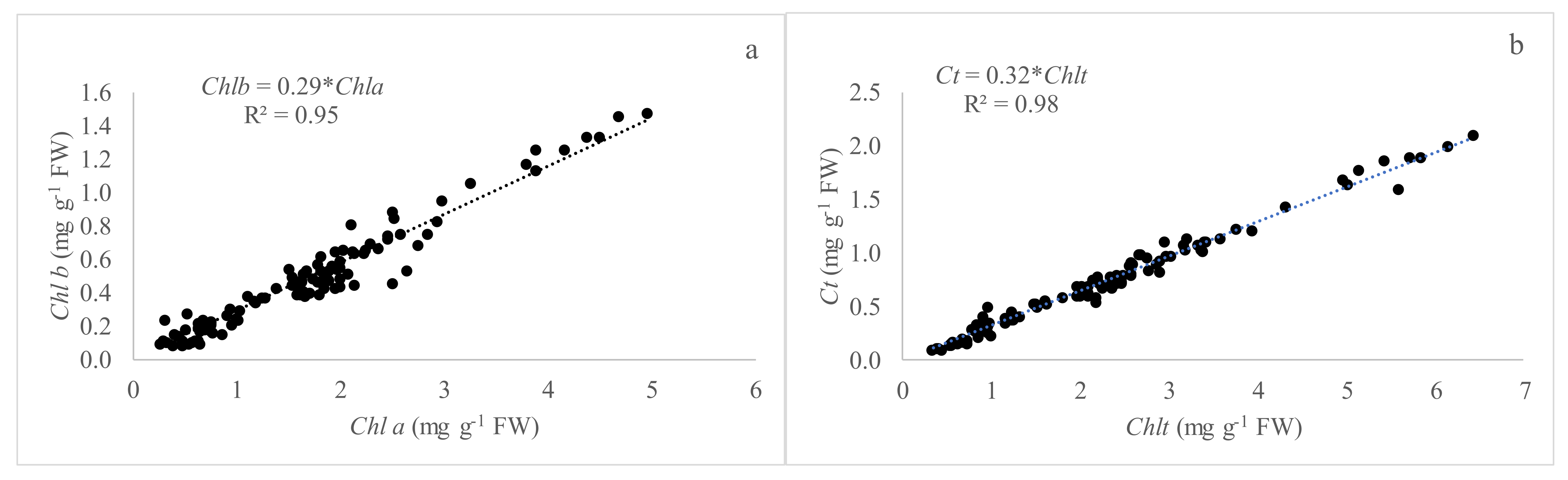
It is necessary to highlight that the carotenoid content does not influence the SPAD readings, according to the principle of this optical measure, but a mathematical relationship between the concentration of carotenoids and the SPAD readings has been studied as an indirect measure since there is a fixed relationship between the Chlt and Carotenoids (Figure 1b and Figure 3b).

The relationship between the average pigments Chl a and b, and the Chlt and Ct corresponding to the whole species studied is showed in Figure 1. It is interesting to note the good and significant (p < 0.05) relationship between the studied variables with values of R² of 0.95 and 0.98, respectively.

3.1.3. Chlorophyll Index and Specific Weight

Table 5. Chlorophyll Index and Specific Weight (mg FW cm⁻²) of all species studied in the first trial. The values in the same column followed by the same letter are not significantly different.

Species	Chlorophyll Index	Specific Weight (mg FW cm−2)
Anthurium scherzerianum	53.74 ± 4.60 bc	28.37 ± 4.49 de
Aspidistra elatior	48.98 ± 7.70 bc	23.10 ± 1.67 f
Begonia sp. “Pink”	35.98 ± 4.29 d	35.11 ± 4.17 c
Begonia sp. ‘White’	38.08 ± 5.07 cd	41.58 ± 7.62 bc
Canna indica	52.30 ± 4.45 bc	26.57 ± 3.18 de
Cissus rhombifolia	46.78 ± 6.70 bc	16.22 ± 1.16 g
Ficus australis	52.16 ± 3.92 bc	55.57 ± 7.40 b
Ficus benjamina	70.50 ± 7.04 ab	20.34 ± 1.30 f
Gerbera sp.	43.46 ± 6.47 cd	20.52 ± 3.33 f
Hedera helix	52.16 ± 8.59 bc	22.03 ± 5.97 def
Hibiscus rosa-sinensis	58.82 ± 6.72 b	30.20 ± 5.34 cd
Impatiens sp.	66.14 ± 8.46 ab	30.07 ± 5.91 d
Monstera deliciosa	76.04 ± 4.80 a	14.50 ± 2.64 g
Nephrolepis exaltata	35.00 ± 4.35 d	15.51 ± 2.12 g
Pelargonium zonale	41.48 ± 1.74 cd	29.23 ± 3.94 de
Philodendron scandens	45.58 ± 4.50 c	53.82 ± 6.17 b
Rumohra adiantiformis	71.35 ± 2.75 a	25.85 ± 3.08 ed
Ruscus aculeatus	60.13 ± 5.55 b	18.81 ± 1.44 g
Schefflera arboricola	72.82 ± 4.01 a	36.30 ± 3.01 c
Syngonium podophillum	43.48 ± 4.43 c	14.36 ± 3.57 g
Tradescantia sillamontana	37.62 ± 9.20 cd	78.70 ± 6.21 a
Tradescantia zebrina	41.78 ± 6.31 cd	78.80 ± 5.34 a
Yucca elephantipes	75.36 ± 7.72 a	82.84 ± 3.50 a

shows the chlorophyll index (CI) measured by SPAD-502 (unitless) and Specific Weight (SW) (mg FW cm⁻²) of all species studied. The Chlorophyll Index varied from 35 to 76 and the Specific Weight varied from 14.36 to 82.84 mg FW cm⁻².

3.1.4. Relationship between SPAD Values (LSPAD) and Pigment Concentrations

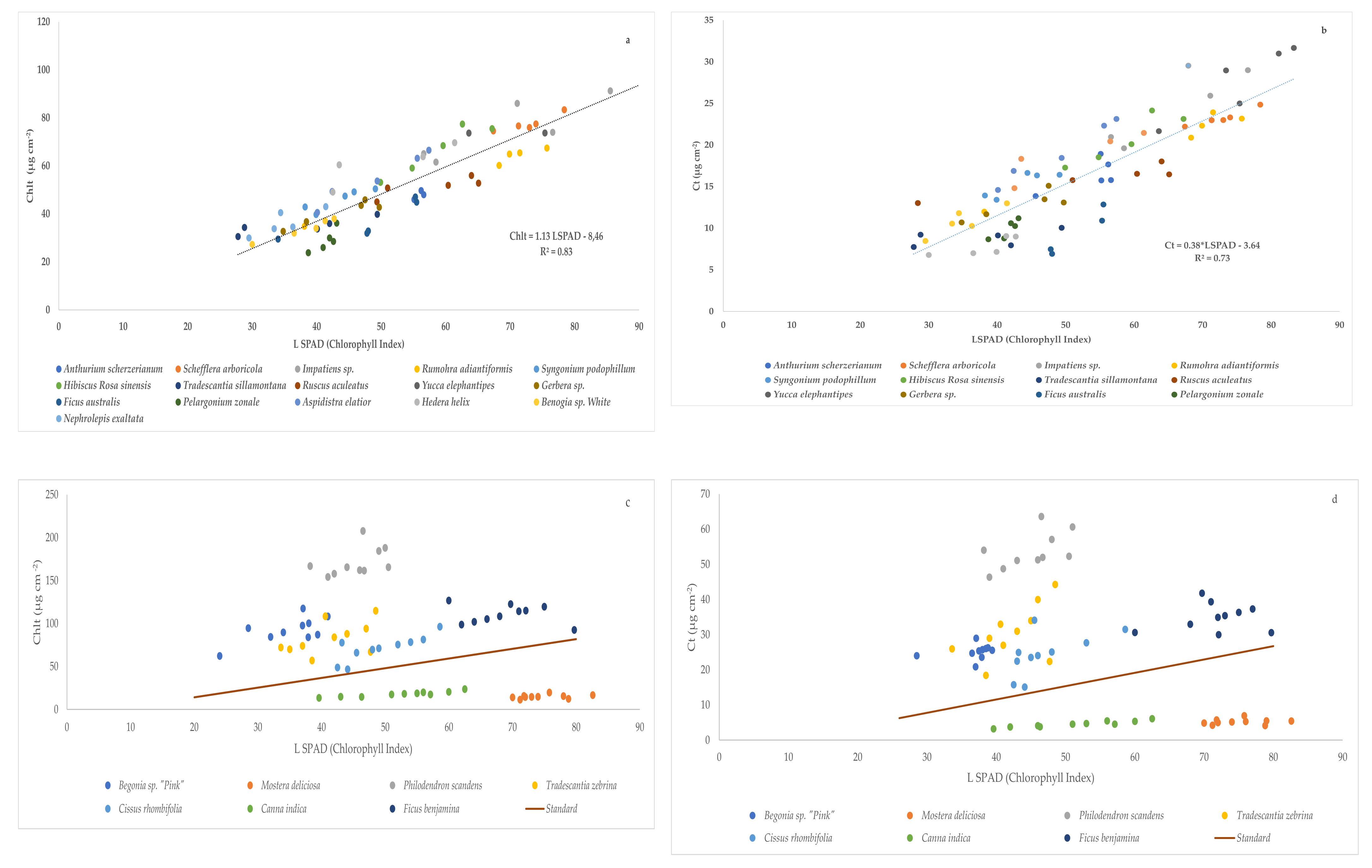
All the species studied in the first trial showed a high value of R² close to 1 and a positive slope for the correlations between chlorophyll index (LSPAD) readings and total chlorophyll (Chlt) and carotenoids (Ct) concentration (

Table 6. Individualized correlation study for each species of the first trial between chlorophyll index (LSPAD) readings and total chlorophyll (Chlt) and carotenoids (Ct) concentration.

	Cht		Ct
Species	Equation	R2	Equation	R2
Anthurium scherzerianum	Cht = 1.35 × LSPAD + 55.91	0.65	Ct = 0.29 × LSPAD + 0.79	0.56
Aspidistra elatior	Cht = 1.43 × LSPAD − 10.61	0.96	Ct = 0.46 × LSPAD − 3.56	0.97
Begonia sp. “Pink”	Cht = 1.88 × LSPAD + 27.18	0.53	Ct = 1.05 × LSPAD − 14.46	0.71
Begonia sp. ‘White’	Cht = 0.93 × LSPAD + 1.93	0.97	Ct = 0.17 × LSPAD + 1.19	0.61
Canna indica	Cht = 0.40 × LSPAD − 2.51	0.88	Ct = 0.11 × LSPAD − 0.99	0.89
Cissus rhombifolia	Cht = 1.84 × LSPAD + 11.28	0.95	Ct = 0.75 × LSPAD − 11.98	0.61
Ficus australis	Cht = 0.88 × LSPAD + 0.32	0.71	Ct = 0.63 × LSPAD − 22.83	0.92
Ficus benjamina	Cht = 1.77 × LSPAD − 7.25	0.78	Ct = 0.32 × LSPAD + 12.20	0.71
Gerbera sp.	Cht = 0.95 × LSPAD + 6.00	0.89	Ct = 0.22 × LSPAD + 3.16	0.72
Hedera helix	Cht = 0.89 × LSPAD + 20.40	0.74	Ct = 0.28 × LSPAD + 4.62	0.79
Hibiscus rosa-sinensis	Cht = 1.49 × LSPAD + 20.22	0.90	Ct = 0.40 × LSPAD − 2.84	0.83
Impatiens sp.	Cht = 1.12 × LSPAD + 11.89	0.75	Ct = 0.47 × LSPAD − 5.94	0.76
Monstera deliciosa	Cht = 0.19 × LSPAD + 0.97	0.43	Ct = 0.28 × LSPAD − 15.16	0.66
Nephrolepis exaltata	Cht = 1.12 × LSPAD + 0.89	0.70	Ct = 0.34 × LSPAD − 1.18	0.77
Pelargonium zonale	Cht = 1.36 × LSPAD − 64.80	0.70	Ct = 0.57 × LSPAD − 13.54	0.76
Philodendron scandens	Cht = 1.69 × LSPAD + 92.41	0.42	Ct = 0.75 × LSPAD + 18.6	0.67
Rumohra adiantiformis	Cht = 1.02 × LSPAD + 0.96	0.99	Ct = 0.32 × LSPAD − 0.05	0.97
Ruscus aculeatus	Cht = 1.03 × LSPAD + 24.86	0.70	Ct = 0.11 × LSPAD + 9.85	0.89
Schefflera arboricola	Cht = 0.87 × LSPAD + 21.37	0.83	Ct = 0.23 × LSPAD + 6.21	0.93
Syngonium podophillum	Cht = 1.12 × LSPAD + 5.83	0.83	Ct = 0.31 × LSPAD + 2.09	0.76
Tradescantiasillamontana	Cht = 1.42 × LSPAD + 23.00	0.74	Ct = 0.05 × LSPAD + 6.76	0.27
Tradescantia zebrina	Cht = 1.79 × LSPAD15.84	0.87	Ct = 1.23 × LSPAD − 15.29	0.68
Yuccaelephantipes	Cht = 1.15 × LSPAD + 1.89	0.92	Ct = 0.50 × LSPAD − 9.94	0.82

).

Figure 2 shows the linear regressions between chlorophyll index (LSPAD) and total chlorophyll concentration (Chlt) (Figure 2a) and carotenoids concentration (Ct) (Figure 2b) of studied species except: Begonia sp. “Pink”, M. deliciosa, P. scandens, T. zebrina, C. rhombifolia, C. indica., and F. benjamina. These species were excluded from the global correlation study because the linear correlation equations found were very different from that obtained with the rest of the species (Table 6 and Figure 2c,d).

3.2. Second Trial at Open Field Conditions (Summer Season)

3.2.1. Pigment Concentrations

Pigment concentrations in plants of different species in the second trial were presented in

Table 7. Pigment concentration (expressed in mg g⁻¹ FW) in plants of different species of the second trial. Data are the means ± standard deviation of five plants per specie (n = 5). The values in the same column followed by the same letter are not significantly different.

Species	Chl a	Chl b	Chlt	Chl a/b Ratio	Carotenoids
Bougainvillea glabra	0.90 ± 0.12 d	0.20 ± 0.03 e	1.10 ± 0.15 d	4.52 ± 0.12 a	0.35 ± 0.04 cd
Clivia miniata	1.07 ± 0.08 cd	0.29 ± 0.03 e	1.36 ± 0.05 d	4.06 ± 0.44 ab	0.40 ± 0.03 c
Hibiscus rosa-sinensis	1.13 ± 0.12 c	0.32 ± 0.05 d	1.45 ± 0.17 d	3.52 ± 0.24 b	0.43 ± 0.04 c
Howea forsteriana	2.91 ± 0.38 a	1.76 ± 0.13 a	4.67 ± 0.35 a	1.65 ± 0.14 f	1.06 ± 0.26 a
Lantana camara	1.43 ± 0.16 b	0.56 ± 0.05 c	1.99 ± 0.19 c	2.56 ± 0.27 d	0.58 ± 0.04 b
Monstera deliciosa	1.19 ± 0.15 c	0.60 ± 0.08 c	1.79 ± 0.22 cd	2.01 ± 0.16 e	0.69 ± 0.09 b
Myoporum laetum	0.59 ± 0.08 e	0.20 ± 0.03 e	0.79 ± 0.10 e	3.04 ± 0.11 c	0.22 ± 0.02 d
Nerium oleander	0.81 ± 0.18 d	0.28 ± 0.12 e	1.10 ± 0.30 d	2.81 ± 0.40 cd	0.31 ± 0.08 d
Philodendron erubescens	1.95 ± 0.11 b	0.99 ± 0.06 b	2.94 ± 0.17 b	1.97 ± 0.07 e	0.90 ± 0.05 a
Schefflera arboricola	1.23 ± 0.08 c	0.91 ± 0.24 b	2.14 ± 0.25 c	1.42 ± 0.38 f	0.59 ± 0.05 b

. The Chl a concentration varied according to the species studied. All values were in the range (0.60–2.91 mg g⁻¹ FW). The highest value was presented for H. forsteriana followed by P. erubescens although not significantly different from and L. camara. Myoporum laetum showed significantly lower values than the rest of the species studied at open field conditions. The opposite results were found in M. deliciosa and S. arboricola.

The Chl b concentration varied also according to the species studied, similar to Chl a results. All values were in the range from 0.20 to 1.76 mg g⁻¹ FW. The highest value was presented for H. forsteriana and the lowest for M. laetum and B. glabra. Chl b concentration was higher under field conditions than greenhouse conditions in the species studied.

The total chlorophyll concentration varied also according to the species studied. All values were in the range from 0.79 to 4.67 mg g⁻¹ FW. The highest value was presented by H. forsteriana; and the lowest value by M. laetum. Chlt concentration was higher under field conditions than greenhouse conditions in H. rosa-sinensis. The opposite results were found in M. deliciosa and S. arboricola.

The carotenoids concentration varied according to the species studied. All values were in the range from 0.22 to 1.06 mg g⁻¹ FW. The highest value was presented by H. forsteriana; and the lowest value by M. laetum. Carotenoid concentration was less under field conditions than greenhouse conditions in H. rosa-sinensis. The opposite results were found in M. deliciosa and S. arboricola.

The highest values of the ratio Chla/Chlb (>4.00) were presented by B. glabra and C. miniata. The lowest values were presented by H. forsteriana and S. arboricola. The other values were comprised from 1.00 to 4.00 mg g⁻¹ FW.

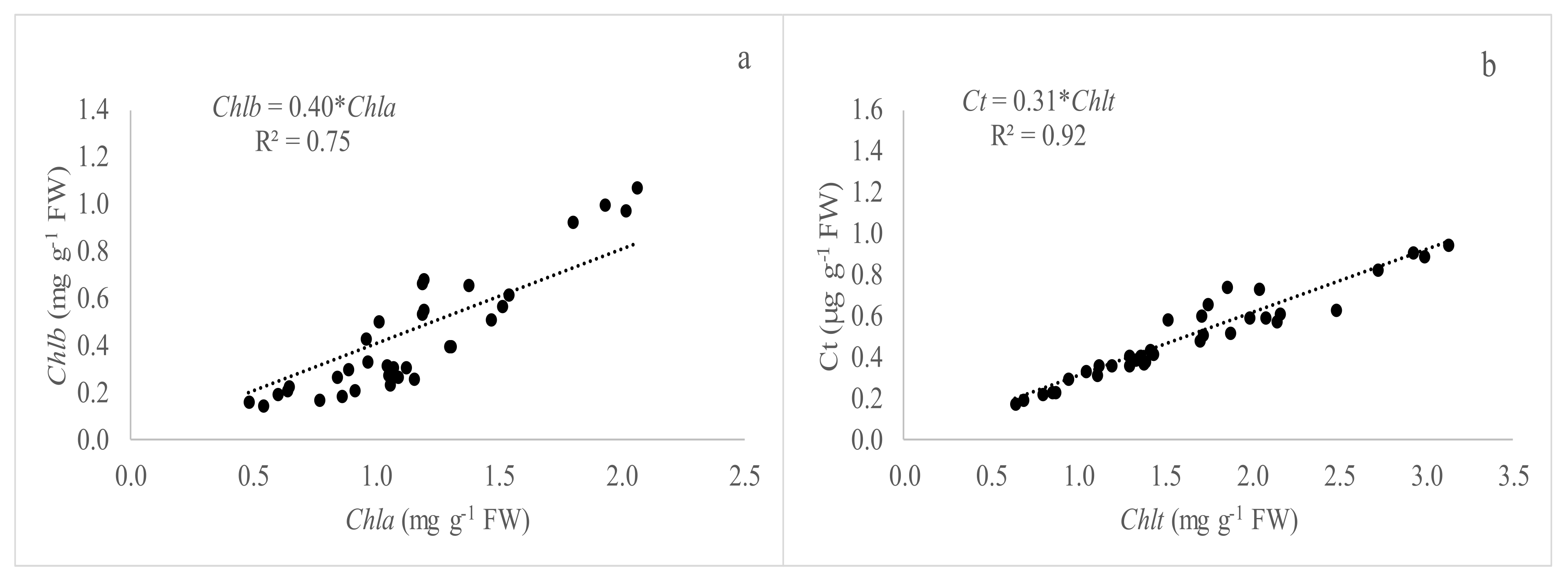
3.2.2. Relationships between the Pigments Analyzed

The relationship between the average pigment concentration (Chl a and b), and Chlt and carotenoids corresponding to all species studied is shown in Figure 3. It is interesting to remark the good and significant (p < 0.05) relationship between the studied variables with values of R² of 0.75 and 0.92, respectively.

3.2.3. Chlorophyll Index and Specific Weight

Table 8. Chlorophyll Index and Specific Weight (mg FW cm⁻²) of all species studied in the second trial. The values in the same column followed by the same letter are not significantly different.

Species	Chlorophyll Index	Specific Weight (mg FW cm−2)
Bougainvillea glabra	66.78 ± 7.90 a	40.18 ± 3.40 b
Clivia miniata	65.90 ± 4.53 a	66.96 ± 4.14 a
Hibiscus rosa-sinensis	55.05 ± 2.35 b	31.12 ± 2.09 b
Howea forsteriana	67.90 ± 7.65 a	14.43 ± 1.11 d
Lantana camara	43.38 ± 1.20 c	21.84 ± 2.14 c
Monstera deliciosa	37.45 ± 1.68 d	17.45 ± 1.65 d
Myoporum laetum	45.60 ± 1.61 c	36.47 ± 2.14 b
Nerium oleander	48.95 ± 4.66 c	34.42 ± 2.15 b
Philodendron erubescens	54.4 ± 2.05 b	24.05 ± 1.80 c
Schefflera arboricola	72.56 ± 4.59 a	37.21 ± 3.20 b

shows the chlorophyll index (CI) measured by SPAD-502 (unitless) and Specific Weight (SW) (mg FW cm⁻²) of all species studied. The Chlorophyll Index varied from 37.45 to 72.56 and the Specific Weight varied from 14.43 to 66.96 mg FW cm⁻².

3.2.4. Relationship between SPAD Values (LSPAD) and Pigment Concentrations

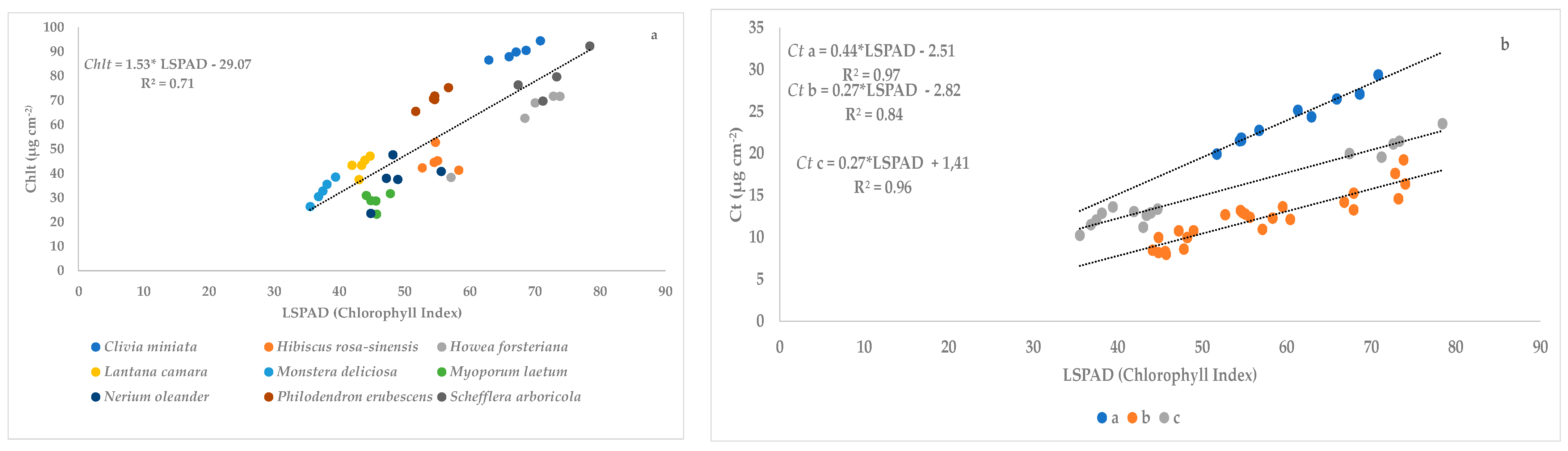
All the species studied in the second trial showed a high value of R² close to 1 and a positive slope for the correlations between chlorophyll index (LSPAD) readings and total chlorophyll (Chlt) and carotenoid (Ct) concentration (

Table 9. Individualized correlation study for each species of the second trial between chlorophyll index (LSPAD) readings and total chlorophyll (Chlt) and carotenoid (Ct) concentration.

	Cht		Ct
Species	Equation	R2	Equation	R2
Bougainvillea glabra	Cht = 0.63 × LSPAD + 1.91	0.70	Ct = 0.18 × LSPAD + 1.60	0.71
Clivia miniata	Cht = 0.98 × LSPAD + 24.15	0.91	Ct = 0.46 × LSPAD − 3.75	0.87
Hibiscus rosa-sinensis	Cht = 2.10 × LSPAD − 83.31	0.74	Ct = 0.97 × LSPAD − 38.87	0.91
Howea forsteriana	Cht = 1.95 × LSPAD − 80.18	0.98	Ct = 0.46 × LSPAD − 16.23	0.86
Lantana camara	Cht = 1.75 × LSPAD − 164.70	0.93	Ct = 0.10 × LSPAD + 8.78	0.99
Monstera deliciosa	Cht = 1.18 × LSPAD − 86.31	0.99	Ct = 0.88 × LSPAD − 21.03	0.99
Myoporum laetum	Cht = 1.25 × LSPAD − 123.57	0.85	Ct = 0.03 × LSPAD + 6.95	0.91
Nerium oleander	Cht = 1.40 × LSPAD + 19.29	0.73	Ct = 0.22 × LSPAD + 0.52	0.98
Philodendron erubescens	Cht = 1.96 × LSPAD − 35.66	0.98	Ct = 0.57 × LSPAD − 9.42	0.99
Schefflera arboricola	Cht = 2.18 × LSPAD − 80.42	0.88	Ct = 0.74 × LSPAD − 30.49	0.73

).

Figure 4 shows the linear regression between SPAD values and total chlorophyll concentration (Chlt) of the studied species except B. glabra (R² = 0.71), because the slope of the equation obtained with this species is very different (0.63 in Table 9). It is interesting to note the highest value of the slope under field conditions. The species showed different trends between Ct concentration and Chlorophyll Index. We established three different groups: (a) C. miniata and P. erubescens (R² = 0.97); (b) B. glabra, H. rosa-sinensis, H. forsteriana, M. laetum and N. oleander (R² = 0.84); and (c) L. camara, M. deliciosa and S. arboricola (R² = 0.96). It is interesting to note the highest value of slope of group a, being even higher than the slope under greenhouse conditions.

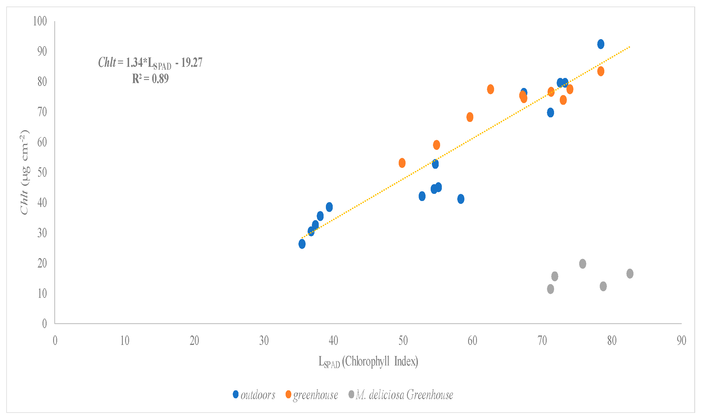
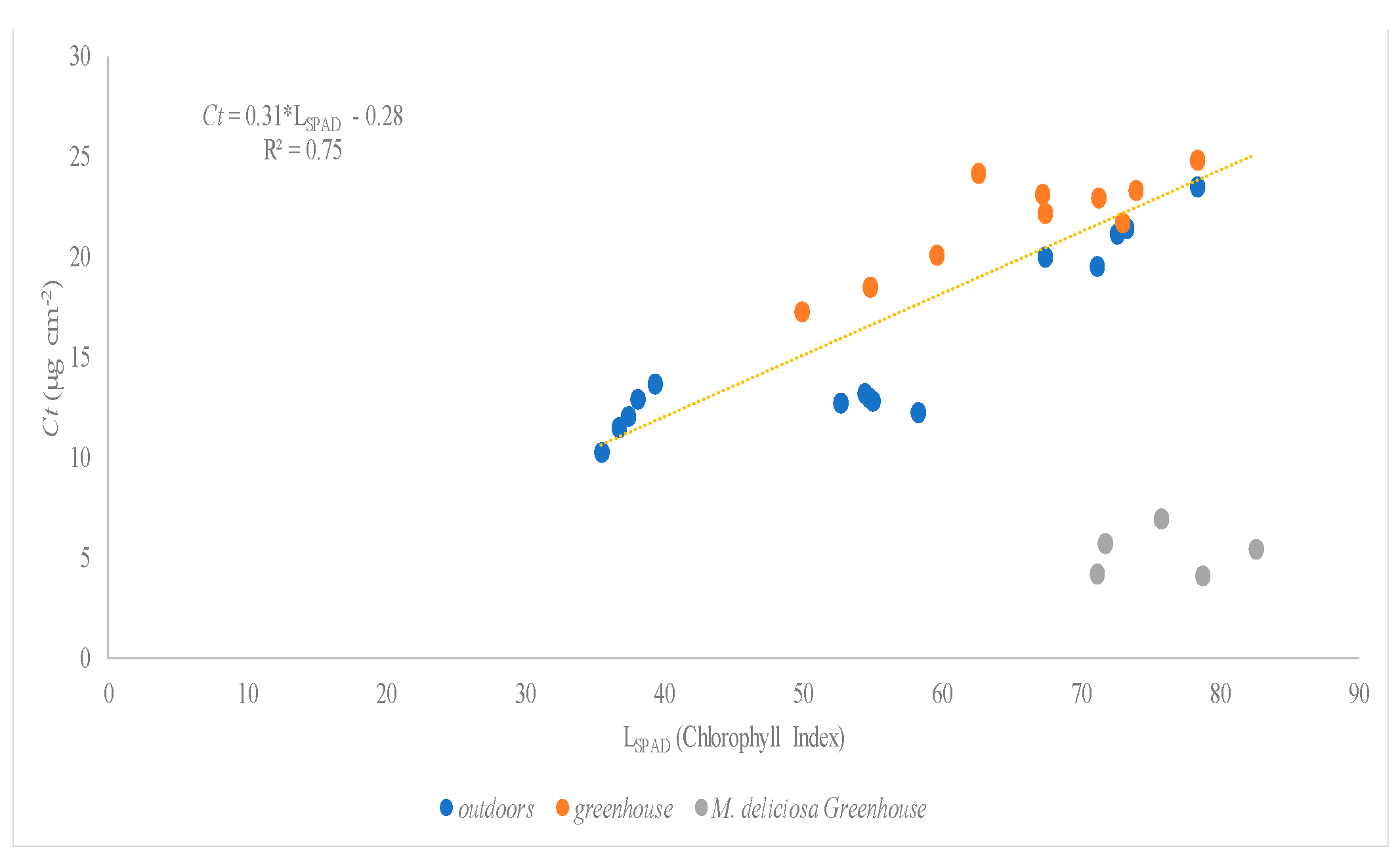
3.3. Relationship between Greenhouse and Outdoor Condition

There were three species assessed under greenhouse and open field conditions: Hibiscus rosa-sinensis, Monstera deliciosa, and Schefflera arboricola. The linear regression between SPAD values and total chlorophyll concentration (Chlt) (Figure 5) and carotenoid concentration (Figure 6) of the studied species showed higher values of R²: 0.89 and 0.75, respectively.

4. Discussion

The chlorophyll content is an important experimental parameter in agronomy and plant biology research [20]. The amount of chlorophyll can vary among the species and also in the same species being related to the levels of irradiance received, plant nutritional status, and stress conditions as well as depending on the genetic factor [21].

It should also be considered that there are a lot of methodologies to determine the chlorophyll concentration in leaf tissues in laboratory: N,N-dimethylformamide (DMF) by Rami and Dan [22]; acetone by Arnon [23]; dimethylsulfoxide (DMSO) by Houborg et al. [24] and methanol, and that the used in this work proposed by Wellburn [19] that offers different values of chlorophyll quantification. In both trials, we used the methodology proposed by Wellburn. This implies that the data of both trials are comparable but should be interpreted if another quantification method has been used.

In our experiment, we found that the Chlt concentration varies significantly between species because plant species (sometimes even within the same plant species) have different pigment concentrations [13]. Comparing the results of both trials, we can see lower values of Chlt in the second trial (summer season) with respect to the first trial (spring season). This fact can be explained by the effects of the high temperature under summer conditions which result in a decrease of photosynthesis rate and consequently in a reduction of pigments concentrations as proposed by Shanmugam et al. [25]. Moreover, higher levels of irradiance at open field conditions (second trial) may be another possible factor responsible for the pigment reduction a result of photooxidative damage [26]. Comparing our results obtained with already published data, the Chlt concentration in C. miniata at field conditions (trial 2) was lower than those reported by Youssef et al. [27] (2.14 mg g⁻¹ FW). Our values in N. oleander were similar to the values proposed by Mugnai et al. [28]. Lower values were found in L. camara (10 times less) than those presented by Singh et al. [29], which can be associated with the use of acetone as extractant. Similar values have been found in N. exaltata compared to the data obtained by Parminder et al. [30].

We examined the relationships between Chla, Chlb, Chlt, and Ct content of the species studied. Not surprisingly, Chla and Chlb were found to be closely associated with each other. In our experiment, the relationships between Chla and Chlb presented a high correlation with values of R² of 0.95 and 0.75 (Figure 1 and Figure 3) and the estimated ratio Chla/Chlb of 3.45 and 2.5 as an inverse of the slope of the regression line, under greenhouse and open field conditions, respectively. In this sense, Shah et al. [14] reported a close relationship between both photosynthetic pigments, Chla being 2–4 times higher than Chlb. The differences in Chla/Chlb ratio depend on several factors like plant species, growth stage, and environmental conditions [31]. It is well known that the Chla/Chlb ratio decreases under shading conditions [32,33]. In the case of the three species that were tested under both conditions, we noted two different trends: H. rosa-sinensis presented similar ratios of Chla/Chlb under both climatic conditions whereas M. deliciosa and S. arboricola decreased their ratios under outdoor conditions. These results agreed with Casierra-Posada et al. [34] who reported in Calendula officinalis a higher Chla/Chlb ratio in leaves under shaded conditions since, under conditions of excess lighting, the photosystem II with a high presence of Chlb is more unstable than photosystem I rich with high presence of Chla. Moreover, PSII is more sensitive to heat stress than PSI; therefore, under heat stress, there is severe damage to the reaction center-binding protein D1 of PSII [35].

In our experiment, the relationships between Chlt and Ct showed values of R² of 0.98 and 0.91 under greenhouse and open field conditions, respectively. The slope was similar under the two assessed conditions (0.32 and 0.31) meaning that the total chlorophyll and carotenoid concentration ratio can be considered constant for all the species studied. This would allow us to make relationships between SPAD readings and carotenoid concentrations assessed. These pigments act as accessory pigments in photosystems and as photoprotective agents reducing the damaging effects of high light [36].

SPAD determinations are widely used to assess the absolute chlorophyll content per leaf area in research settings and agricultural systems [13]. The relationship between Chlorophyll index or SPAD readings and Chlt content has been widely studied in different species such as Euphorbia pulcherrima [37], Elaies guineensis [38] and Fraxinus chinensis, Ginkgo biloba, and Magnolia denudata [39], between others, where there was a good correlation between both parameters when the readings of SPAD oscillated from 26 to 60 and also in the functioning of the chlorophyll extraction procedure assessed. Comparing the results obtained in our experiment with the previous literature, we can report that higher values of chlorophyll Index or SPAD readings were found in F. benjamina under greenhouse conditions and S. arboricola under open field conditions than those reported by Sardoei et al. [40], but under greenhouse conditions, the value of CI in S. arboricola reported by them was similar to our results. We also noted higher SPAD values (66.0) than those found by Massa et al. [41] in Impatiens sp. Nevertheless, the values reported by Parminder et al. [29] in N. exaltata agree with our results. The fitting of our data in both trials reported a linear relationship and values of R² close to 1 between chlorophyll index (LSPAD) readings and total chlorophyll (Chlt) and carotenoids (Ct) concentration. In this sense, Campbell et al. [42] also found a linear model of SPAD–chlorophyll relationships between different experiments and environmental conditions. Nevertheless, Houborg et al. [24] fitted an exponential model to the relationship between SPAD readings and dimethylsulfoxide (DMSO) extractable Chlt per leaf area.

Reviewing previous literature, there are scarce references about the relationship between SPAD-readings and carotenoid concentration. For instance, Shah et al. [14] found a linear relationship in Triticum aestivum with a slope of 0.12 and a coefficient of determination (R²) on 0.85. In our experiment, we also noted a linear relationship between SPAD readings and Ct content per leaf area under greenhouse conditions with a slope of 0.38 and R² of 0.73 and at open field conditions with slope values ranging from 0.27 to 0.44 and values of R² ranging from 0.84 to 0.97. These differences in slope and values of R² can be ascribed to leaf anatomical modifications which may alter the spectral response and SPAD readings [43]. However, in this specific study, the changes found in the regression coefficients of the fitted models did not vary significantly.

In our experiment, the three species studied in both growing conditions (greenhouse and open field conditions) have also been assessed to discern the relationships between chlorophyll index (LSPAD) readings and total chlorophyll (Chlt) and carotenoid (Ct) concentration. The results obtained reported that there are two species H. rosa-sinensis and S. arboricola, whose results obtained for the values of the content in Chlt and Ct conform to the same model of correlation with SPAD in both conditions of cultivation. On the contrary, the species, M. deliciosa, shows very different correlations between these values in both conditions of cultivation, the correlation obtained in the greenhouse being significantly different from the general correlation. These results depicted that these relationships between pigments and SPAD readings can vary among the species due to several factors like leaf optical properties [21].

5. Conclusions

Based on the results obtained, we can report that there was a highly linear relationship between the concentrations of Chla and Chlb, as well as between Chlt and Ct in the different species studied under greenhouse and open field conditions. The ratio between Chla and Chlb was higher at open field conditions and similar between Chlt and Ct. There was also a good relationship between Chlorophyll index and Chlt under both growing conditions, as well as between Chlorophyll index and Ct under greenhouse conditions. However, linear relationships with different slopes were observed for groups of species in open field conditions. Considering the different growing conditions assessed (greenhouse conditions in spring season and open field conditions in summer season), we believe that, through the models provided, the concentration of Chlt and Ct can be estimated with SPAD readings for the species studied.

References

- Liew, W.; Ching, P. Signature optical cues: Emerging technologies for monitoring plant health. Sensors 2008, 8, 3205–3239. [Google Scholar] [CrossRef] [Green Version]
- Chen, M. Chlorophyll modifications and their spectral extension in oxygenic photosynthesis. Annu. Rev. Biochem. 2014, 83, 317–340. [Google Scholar] [CrossRef] [PubMed]
- Tanaka, R.; Tanaka, A. Chlorophyll cycle regulates the construction and destruction of the light-harvesting complexes. Biochim. Biophys. Acta (BBA)-Bioenerg. 2011, 1807, 968–976. [Google Scholar] [CrossRef] [PubMed] [Green Version]
- Pareek, S.; Sagar, N.A.; Sharma, S.; Kumar, V.; Agarwal, T.; González-Aguilar, G.A.; Yahia, E.M. Chlorophylls: Chemistry and biological functions. Fruit Veg. Phytochem. 2017, 29, 269–284. [Google Scholar]
- Holt, N.E.; Zigmantas, D.; Valkunas, L.; Li, X.P.; Niyogi, K.K.; Fleming, G.R. Carotenoid cation formation and the regulation of photosynthetic light harvesting. Science 2005, 307, 433–436. [Google Scholar] [CrossRef] [PubMed] [Green Version]
- Bouvier, F.; Isner, J.C.; Dogbo, O.; Camara, B. Oxidative tailoring of carotenoids: A prospect towards novel functions in plants. Trends Plant Sci. 2005, 10, 187–194. [Google Scholar] [CrossRef] [PubMed]
- Biswal, B. Carotenoid catabolism during leaf senescence and its control by light. J. Photochem. Photobiol. B Biol. 1995, 30, 3–13. [Google Scholar] [CrossRef]
- Peng, S.; Garcia, F.V.; Laza, R.C.; Sanico, A.L.; Visperas, R.M.; Cassman, K.G. Increased n-use efficiency using a chlorophyll meter on high-yielding irrigated rice. Field Crops Res. 1996, 47, 243–252. [Google Scholar] [CrossRef]
- Markwell, J.; Osterman, J.C.; Mitchell, J.L. Calibration of the Minolta SPAD-502 leaf chlorophyll meter. Photosynth. Res. 1995, 46, 467–472. [Google Scholar] [CrossRef]
- Ahmed, S.U. Effects of soil water deficit on leaf nitrogen, chlorophylls and SPAD chlorophyll meter reading on growth stages of soybean. Bangladesh J. Bot. 2011, 40, 171–175. [Google Scholar] [CrossRef] [Green Version]
- Barutcular, C.; Toptas, I.; Turkten, H.; Yildirim, M.; Mujde, K.O.C. SPAD greenness to estimate genotypic variation in flag leaf chlorophyll in spring wheat under Mediterranean conditions. Turk. J. Field Crops 2015, 20, 1–8. [Google Scholar] [CrossRef] [Green Version]
- Jiang, C.; Johkan, M.; Hohjo, M.; Tsukagoshi, S.; Maruo, T.A. Correlation analysis on chlorophyll content and SPAD value in tomato leaves. Hortic. Res. 2017, 71, 37–42. [Google Scholar]
- Uddling, J.; Gelang-Alfredsson, J.; Piikki, K.; Pleijel, H. Evaluating the relationship between leaf chlorophyll concentration and spad-502 chlorophyll meter readings. Photosynth. Res. 2007, 91, 37–46. [Google Scholar] [CrossRef] [PubMed]
- Shah, S.H.; Houborg, R.; McCabe, M.F. Response of chlorophyll, carotenoid and SPAD-502 measurement to salinity and nutrient stress in wheat (Triticum aestivum L.). Agronomy 2017, 7, 61. [Google Scholar] [CrossRef] [Green Version]
- García-Caparrós, P.; Lao, M.T. The effects of salt stress on ornamental plants and integrative cultivation practices. Sci. Hortic. 2018, 240, 430–439. [Google Scholar] [CrossRef]
- Wang, Q.; Chen, J.; Li, Y. Nondestructive and Rapid Estimation of Leaf Chlorophyll and Nitrogen Status of Peace Lily Using a Chlorophyll Meter. J. Plant Nutr. 2004, 27, 557–569. [Google Scholar] [CrossRef]
- Wang, Q.; Chen, J.; Stamps, R.H.; Li, Y. Correlation of Visual Quality Grading and SPAD Reading of Green-Leaved Foliage Plants. J. Plant Nutr. 2005, 28, 1215–1225. [Google Scholar] [CrossRef]
- Jiménez, R.; Caballero, M. El Cultivo Industrial de Plantas en Maceta; Ediciones De Horticultura S.L.: Reus, Spain, 1990; p. 664. [Google Scholar]
- Wellburn, A. The spectral determination of chlorophylls a and b, as well as total carotenoids, using various solvent with spectrophotometers of different resolution. J. Plant Physiol. 1994, 144, 307–313. [Google Scholar] [CrossRef]
- Lamb, J.J.; Eaton-Rye, J.J.; Hohmann, M.F. An LED-based fluorometer for chlorophyll quantification in the laboratory and in the field. Photosynth. Res. 2012, 114, 59–68. [Google Scholar] [CrossRef] [PubMed]
- Sevik, H.; Karakas, H.; Karaca, U. Color-chlorophyll relationship of some indoor ornamental plants. Int. J. Engin. Sci. Res. Techol. 2013, 2, 1706–1712. [Google Scholar]
- Rami, M.; Dan, P. Chlorophyll determination in intact tissues using N,N-Dimethylformamide. Plant Physiol. 1980, 65, 478–479. [Google Scholar]
- Arnon, D. Copper enzymes isolated chloroplasts, polyphenol oxidase in Beta vulgaris. Plant Physiol. 1949, 24, 478–479. [Google Scholar] [CrossRef] [Green Version]
- Houborg, R.; Anderson, M.; Daughtry, C. Utility of an image-based canopy reflectance modeling tool for remote estimation of LAI and leaf chlorophyll content at the field scale. Remote Sens. Environ. 2009, 113, 259–274. [Google Scholar] [CrossRef]
- Shanmugam, S.; Kjaer, K.H.; Ottosen, C.O.; Rosenqvist, E.; Kumari Sharma, D.; Wollenweber, B. The alleviating effect of elevated CO2 on heat stress susceptibility of two wheat (Triticum aestivum L.) cultivars. J. Agron. Crop Sci. 2013, 199, 340–350. [Google Scholar] [CrossRef]
- Foyer, C.H.; Lelandais, M.; Kunert, K.J. Photooxidative stress in plants. Physiol. Plant. 1994, 92, 696–717. [Google Scholar] [CrossRef]
- Youssef, A.S.M.; Ismaeil, F.H.M. Response of Clivia miniata plant to light intensity and kinetin treatments. Ann. Agric. Sci. 2009, 47, 149–164. [Google Scholar]
- Mugnai, S.; Pardossi, A.; Serra, G.; Tognoni, F. Leaf water relations and gas exchange in container-grown plants of two genotypes of Nerium oleander L. as affected by water deficiency. Adv. Hortic. Sci. 1995, 9, 27–32. [Google Scholar]
- Singh, N.; Shrivastava, R.; Mishra, A. Influence of leaf dust deposition on chlorophyll content of Bougainvillea spectabilis and Lanatana camara growing in vicinity of jaypee cement plant, rewa (mp). Int. J. Inf. Res. Rev. 2018, 5, 5685–5688. [Google Scholar]
- Parminder, S.; Dubey, R.K.; Kushal, S. Effect of shade levels on growth and frond production in boston fern Nephrolepis exaltata (L.) Schott. Asian J. Hortic. 2014, 9, 377–381. [Google Scholar]
- Kitajima, K.; Hogan, K.P. Increases of chlorophyll a/b ratios during acclimation of tropical woody seedlings to nitrogen limitation and high light. Plant Cell Environ. 2003, 26, 857–865. [Google Scholar] [CrossRef] [PubMed]
- Salisbury, F.B.; Ross, C.W. Plant Physiology; Wadsworth Publishing Company: Belmont, CA, USA, 1991; 682p. [Google Scholar]
- Dale, M.P.; Causton, D.R. Use of the chlorophyll a/b ratio as a bioassay for the light environment of a plant. Funct. Ecol. 1992, 6, 190–196. [Google Scholar] [CrossRef]
- Casierra-Posada, F.; Ávila-León, O.; Riascos-Ortíz, D. Cambios diarios del contenido de pigmentos fotosintéticos en hojas de caléndula bajo sol y sombra. Temas Agrar. 2012, 1, 60–71. [Google Scholar] [CrossRef] [Green Version]
- Yan, K.; Chen, P.; Shao, H.; Shao, C.; Zhao, S.; Brestic, M. Dissection of photosynthetic electron transport process in sweet sorghum under heat stress. PLoS ONE 2013, 8, e62100. [Google Scholar] [CrossRef] [PubMed] [Green Version]
- Johnson, G.N.; Scholes, J.D.; Horton, P.; Young, A.J. Relationships between carotenoid composition and growth habit in British plant species. Plant Cell Environ. 1993, 16, 681–686. [Google Scholar] [CrossRef]
- Dunn, B.L.; Singh, H.; Goad, C. Relationship between chlorophyll meter readings and nitrogen in poinsettia leaves. J. Plant Nutr. 2018, 41, 1566–1575. [Google Scholar] [CrossRef]
- Sim, C.C.; Zaharah, A.R.; Tan, M.S.; Goh, K.J. Rapid determination of leaf chlorophyll concentration, photosynthetic activity and NK concentration of Elaies guineensis via correlated SPAD-502 chlorophyll index. Asian J. Agric. Res. 2015, 9, 132–138. [Google Scholar]
- Li, J.; Zhou, X.; Zhou, J.; Shang, R.; Wang, Y.; Jing, P. Comparative Study on Several Determination Methods of Chlorophyll Content in Plants. In Proceedings of the 2019 6th Annual International Conference on Material Engineering and Application, Guangzhou, China, 20–21 December 2019; IOP Conference Series: Materials Science and Engineering. IOP Publishing: Beijing, China, 2020; Volume 730, p. 012066. [Google Scholar]
- Sardoei, A.S.; Rahbarian, P.; Shahdadneghad, M. Evaluation chlorophyll contents assessment on three indoor ornamental plants with plant growth regulators. Eur. J. Exper. Biol. 2014, 4, 306–310. [Google Scholar]
- Massa, D.; Prisa, D.; Lazzereschi, S.; Cacini, S.; Burchi, G. Heterogeneous response of two bedding plants to peat substitution by two green composts. Hortic. Sci. 2018, 45, 164–172. [Google Scholar] [CrossRef]
- Campbell, E.E.; Knoop, W.T.; Bate, G.C. A comparison of phytoplankton biomass and primary production in three eastern cape estuaries, South Africa. S. Afr. J. Sci. 1991, 87, 259–264. [Google Scholar]
- Zhu, J.; Tremblay, N.; Liang, Y. Comparing SPAD and at leaf values for chlorophyll assessment in crop species. Can. J. Soil Sci. 2012, 92, 645–648. [Google Scholar] [CrossRef]
Figure 1.
Relationship between pigments of all species studied under greenhouse conditions (spring season). (a) linear relationship between chla and chlb (n = 70); (b) linear relationship between Chlt and Ct (n = 70).
Figure 2.
Relationship between SPAD-502 readings (LSPAD) and the pigments concentration of the studied species: (a) SPAD-502 vs. total chlorophyll concentration (Chlt, µg cm−2); (b) SPAD-502 vs. carotenoid concentration (Ct µg cm−2), (c) SPAD-502 vs. total chlorophyll concentration (Chlt, µg cm−2) of excluded species with the standard regression (Figure 2a). (d) SPAD-502 vs. carotenoid concentration (Ct µg cm−2) of excluded species with the standard regression (Figure 2b). The linear curve was fitted in both cases.
Figure 3.
Relationship between pigments concentration of all species under field conditions (summer season). (a) linear relationship between chl a and chl b (n = 50); (b) linear relationship between Chlt and Ct (n = 50).
Figure 4.
Relationship between SPAD-502 readings (LSPAD) and the pigments of studied species: (a) SPAD-502 vs. total chlorophyll contents (Chlt µg cm−2), (b) SPAD-502 vs. carotenoid concentration (Ct µg cm−2). A linear curve was fitted in both cases.
Figure 5.
Relationship between SPAD values (LSPAD) and total chlorophyll concentration (Chlt µg cm−2) of Hibiscus rosa-sinensis, Monstera deliciosa, and Schefflera arboricola.
Figure 6.
Relationship between SPAD values (LSPAD) and carotenoid concentration (Ct µg cm−2) of Hibiscus rosa-sinensis, Monstera deliciosa, and Schefflera arboricola.