1. Introduction
Global Navigation Satellite Systems (GNSS) allow the determination of the 3D position of a point on the Earth’s surface (constituted by its geodetic coordinates, i.e., longitude, latitude and altitude), by using the signal code and/or carrier phase and, therefore, measuring the distance (pseudorange) from the receiver antenna to the orbital position of at last four satellites within a certain time [
1,
2,
3]. The main satellite constellations from which the antenna of the different GNSS receivers can receive the signals are GPS (Global Positioning System), operated by US Department of Defence and using 31 satellites; GLONASS (GLObal NAvigation Satellite System), operated by the Russian Federation and using 23 satellites; BeiDou, operated by China and using 49 satellites; EGNOS (European Geostationary Navigation Overlay Service), SBAS (Satellite-Based Augmentation System) developed by the European Space Agency (ESA) under the Galileo project and using 22 satellites; QZSS (Quasi-Zenith Satellite System) or MSAS (Multi-functional Satellite Augmentation System), SBAS operated by Japan and using 4 satellites.
A GNSS to be used must be economically viable and, depending on the crop and on the cultivated area, achieve high values of precision and accuracy. The accuracy is the difference between the measured value of a quantity and the real one, so the positioning accuracy of a GNSS is the distance between the position of a point on the Earth’s surface determined by this system and the real one [
4]. The precision is, however, the statistical dispersion degree of computed data with reference to their mean, i.e., their standard deviation with reference to the mean of the sample [
5]. GNSS can often determine the position of a point with a positioning accuracy which is better than 1 m, even if this accuracy can be improved through the reception of differential correction signals, in real time or in post-processing [
4]. The process for achieving positioning accuracy up to one centimetre in GNSS involves a complex algorithm known as Real-Time Kinematic (RTK) or Dynamic processing [
6]. RTK-capable receivers must be connected to precisely calibrated antennas, for processing the signals transmitted by GNSS satellites, and receive and process differential correction data from a ground network of stations [
7] or from a single reference station. In fact, the EUREF Permanent Network (EPN), built up in 1996, is a science-driven network of GNSS Continuously Operating Reference Stations (CORS) covering Europe. The EPN, having the task of maintaining the European Terrestrial Reference System 89 (ETRS89), monitors the geodetic coordinates of its tracking stations with a level of accuracy of less than one centimetre [
8]. A few years ago, RTK-capable receivers were expensive and bulky. Therefore, recently, GNSS receiver manufacturers have started marketing cheap and compact RTK-capable receivers [
7].
Dual-frequency (L1/L2) GNSS receivers for geodetic surveying are able to achieve up to a one millimetre level of accuracy, but at the moment, they are expensive (at least €3700) [
9].
Nowadays, survey-grade dual-frequency RTK-capable GNSS receivers must be used for determining a 3D trajectory with a level of accuracy of up to one centimetre during kinematic (RTK) applications, e.g., in precision agriculture, only for the control and guidance of agricultural machines. The majority of users have low-cost GNSS receivers, which are small and easy to handle and embed. These receivers are also capable of being used in RTK positioning mode with a level of accuracy of up to one centimetre. However, most low-cost receivers are only single frequency (L1). The open-source program package RTKLIB, that was developed by Takasu and Yasuda [
10], can be used by low-cost receivers for RTK mode [
9].
To date, only very few researchers have focused on dynamic (RTK) applications of low-cost L1 frequency receivers, e.g., Takasu and Yasuda [
10].
A low-cost approach requires the following components: (1) L1 GNSS board; (2) L1 GNSS antenna; (3) reference data, i.e., RTCM (Radio Technical Commission for Maritime Services) differential correction data from L1 local CORS, e.g., via NTRIP (Networked Transport of RTCM via Internet Protocol) or from L1/L2 base station; (4) PC, running an RTK GNSS software for positioning [
11].
Procedures for evaluating the results of L1 RTK-capable GNSS receivers were carried out for the first time by Stempfhuber and Buchholz [
11]. These receivers were able to calculate 3D positions with a level of accuracy of one centimetre [
12]. The use of local L1 reference information is the most cost-effective approach for low-cost RTK GNSS applications [
11].
Following the implementation of GNSS in agriculture, a slow change of applied technologies, based on the geo-referenced measurement of within-field crop and soil parameters, is in progress, allowing for more effective crop input management. This new approach, which is achieving great success worldwide, is known as precision agriculture or precision farming. The low-cost implementation of these technologies can increase their use and make spatially variable crop input management more effective [
4].
Even though precision agriculture was implemented for the first time in US at the beginning of 1980s, it is currently widespread only in large areas of US, Germany, Denmark, Netherlands and United Kingdom [
13]. Moreover, precision agriculture is spreading slowly in Italy (where it is currently implemented in only 1% ca. of cultivated area), above all due to farmers’ resistance to investment in manpower and capital without knowing if this will provide a significantly higher profit [
14].
Different studies [
15,
16,
17] have proved the economic benefits of precision agricultural technologies. The capital to be invested for implementing precision agriculture is variable from €2500 to €50,000. The implementation of precision agriculture requires the investment of fixed capital, for buying suitable agricultural machines and/or parts of them (e.g., aided guidance system, satellite antenna, GNSS receiver, monitor) and related software [
18]. This increases the depreciation charge and, therefore, the fixed costs. However, precision agriculture influences the cost of using agricultural machines by causing the reduction of variable costs proportional to their use: fuels, oil, maintenance and insurance. This reduction of the cost of using agricultural machines is variable, depending on the technologies implemented and the regularity or irregularity of fields and cultivated crops.
The first step for implementing precision agriculture is buying a GNSS receiver, which should be selected depending on farm needs. In fact, sometimes a low-cost GNSS receiver can provide the farmer with a higher profit, i.e., if an agricultural implement with a high working width is used for soil tillage or an agricultural machine is used for a crop operation requiring a maximum error of 0.3 m (e.g., fertiliser application). On the contrary, when a tractor is used for high-accuracy crop operations (e.g., soil tillage of row crops, strip tillage, pesticide spraying, hoeing) a survey-grade RTK-capable GNSS receiver is needed. A positioning accuracy level of 10–30 mm is needed within precision agriculture, for the control and guidance of agricultural machines [
11].
GNSS receivers are included in the aided guidance systems of agricultural machines. For instance, a study carried out on corn crop showed that the cost of using agricultural machines decreases 29.37 €/ha when replacing manual tractor guidance with an automatic one [
18].
It is possible to distinguish between three types of aided guidance systems of agricultural machines: manual; semiautomatic; automatic.
In the manual guidance system, the steering wheel is operated by the driver by relying on the information provided by a LED light bar or a monitor placed on the dashboard and indicating the corrections to be carried out (turn left or right). This system allows constant forward speed and better accuracy and, therefore, more regular trajectories.
In the semiautomatic guidance system, during travel road, the driver normally operates the steering wheel. During a crop operation, on the other hand, an electrical wheel is able to move the steering wheel. This system allows the driver to pay attention to the working quality of the agricultural implement and to increase the forward speed by 10–15% for some crop operations (e.g., soil tillage, hoeing, sowing).
In the automatic guidance system, during a crop operation, a control unit manages the steering wheel, the gearbox, the hydraulic lift and the connected agricultural machine or implement.
The aided guidance system is offered by the manufacturer of agricultural machines or is sold by the manufacturer of GNSS receivers or specialized companies (e.g., AvMap, AgLeader) as part of the tractor or to be mounted on the tractor owned by the farmer. In many cases, it is an all-in-one system, including GNSS receiver and monitor, while it is sometimes a more complex system consisting of a GNSS receiver, monitor, actuator, controller for spatially variable rate crop input application, etc. [
19,
20,
21,
22]. A low-cost solution available online for building up a homemade automatic guidance system is offered by AgOpenGPS project, which provides the outlines and designs of the hardware to be developed, as well as the software that is distributed together with GNU (General Public) license.
The aim of this work is to compare the positioning accuracy of four GNSS receivers having different technical features and working modes, from a dual-frequency (L1/L2) survey-grade RTK-capable receiver to a low-cost single frequency (L1) GPS receiver.
2. Materials and Methods
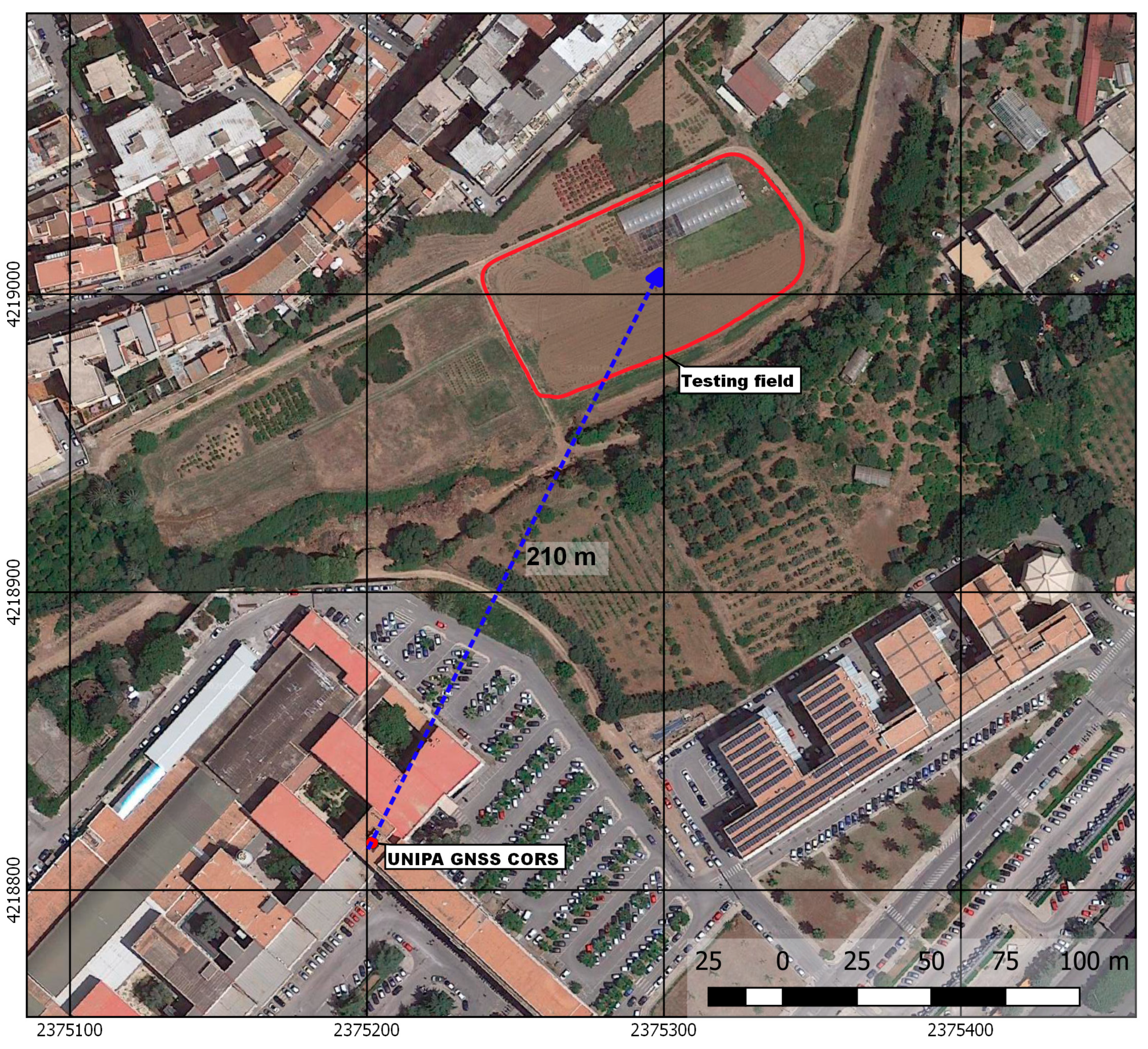
2.1. Testing Field
The tests were carried out in the campus area of the University of Palermo (13°20’58.21” E; 38°6’25.99” N; 31 m a.s.l.), along the edge of a flat field, with a perimeter of 287 m and an area of 4350 m
2, divided into different experimental parcels (
Lolium perenne L. and
Poa pratensis L. turf; officinal plants
Salvia officinalis L., Rosmarinus officinalis L.). The soils have a sandy clayey texture: Aric Regosol, 54% sand, 23% silt and 23% clay (CIT). The general features of the testing field can be observed in
Figure 1.
2.2. Tested Satellite Receivers
Four GNSS receivers were used: Stonex S7-G; Stonex S5; Thales MobileMapper Pro; Quanum GPS Logger V2 (U-Blox NEO-6M).
The satellite receiver Stonex S7-G (named S7) is able to receive L1 (1575.42 MHz) and L2 (1227.60 MHz) signals from GPS, GLONASS, BeiDou and SBAS (e.g., EGNOS) satellites; it has 120 channels, a maximum position update rate of 5 Hz (5 positions s−1), a size of 234 × 99 × 56 mm and a weight (without battery) less than 900 g, and it is also powered by a battery of 11.1 V and 2500 mA. The internal antenna has a choke ring which can suppress multipath satellite signals. This receiver is equipped with a Cortex-A8-AM33X processor with a frequency of 1 GHz, internal memory of 8 GB, external memory of 8 GB on SD board and RAM of 512 MB, as well as working with a Windows Mobile 6.5 Professional operating system. The receiver S7-G is also equipped with a slot for a SIM card and a GSM/GPRS/EDGE modem, which allows a quick and effective Internet connection, in order to obtain differential correction data in real time from the network of RTK ground stations (CORS). This receiver is equipped with Wi-Fi and Bluetooth connections, as well as a high brightness colour TFT display Blanview 480 × 640 VGA, allowing an interface with the measured or previously logged data, by providing the user with excellent visibility of the field work. This instrument is also equipped with a camera with a resolution of 5 MPixel and autofocus. The horizontal (2D, longitude and latitude) accuracy specified by the manufacturer is 5 mm + 1 ppm rms (root mean square, i.e., 63–68% of measurements) in static (stand-alone) mode, 0.6 m rms by using SBAS satellites, 0.4 m rms in differential mode (only code), 20 mm + 1 ppm in RTK mode with internal antenna, 10 mm + 1 ppm in RTK mode with external antenna.
The satellite receiver Stonex S5 (named S5) is able to receive only L1 signal from GPS, GLONASS, BeiDou, QZSS and SBAS satellites; it has 372 channels, a maximum position update rate of 20 Hz (20 positions s−1), a size of 119 × 86 × 32 mm and a weight (without battery) of 290 g, and it is powered by a battery of 3.7 V and 3700 mA. This receiver is able to receive differential correction signals through Bluetooth and Wi-Fi connections, in order to reduce the positioning error, and is equipped with an AM355X processor, having a memory of 4 GB and RAM of 512 MB and working with a Linux operating system. The horizontal accuracy specified by the manufacturer is 1.2 m rms in static mode, 0.6 rms by using SBAS satellites, 0.5 m CEP (Circular Error Probable, i.e., 50% of measurements) in differential mode (only code), less than 0.5 m + 1 ppm by using post-processed differential correction data and 0.3-0.6 m by using differential correction data from CORS.
The low-cost hand-held satellite receiver Thales MobileMapper Pro (named TMMP) allows the determination of the geodetic coordinates of a point and transfer of them to Geografic Information System (GIS) software; it has 12 channels, a position update rate of 1 Hz (1 position s−1), a size of 16.5 × 7.4 × 3.05 cm and a weight (with batteries) of 227 g, and is powered by two AA batteries. This receiver is equipped with a multipath-resistant internal antenna. An SD board can be inserted into this receiver in order to log a high amount of data. By means of this receiver, it is possible to perform the differential correction only in post-processing. This instrument is able to receive only an L1 signal from GPS and SBAS satellites. The horizontal accuracy specified by the manufacturer is 7 m 2drms (2 distance rms, i.e., 95% of measurements) in static mode, 0.7 m 2drms by using post-processed differential correction data, 2–3 m 2drms by using real-time differential correction data from EGNOS or land-based systems, e.g., a private broadcast via RTCM (Type 1 or 9) standard.
The low-cost satellite receiver assembled at the Department of Agricultural, Food and Forest Sciences (SAAF) of the University of Palermo, Quanum GPS Logger V2 (named QLV2), with built-in GPS U-Blox NEO-6M receiver, is an autonomous device receiving energy from a reserved channel so that it needs no additional battery. This receiver has 50 channels, a position update rate of 1 Hz (1 position s−1), a size of 24 × 77 × 18 mm and a weight (without battery) of 43 g, and is powered by an external battery and is able to log travelled distance, starting and ending position of a route, date, UTC (Universal Time Coordinated), route and speed (also the maximum one). The data can be shown on the built-in backlighted LCD display. The differential correction data in NMEA (National Marine Electronics Association) standard can be easily downloaded to a PC so that the positions can be displayed in mapping websites (e.g., Google Earth). This instrument is able to receive only L1 signal (C/A code) from GPS and SBAS satellites (via NMEA 0183 V 4.10 standard). The accuracy specified by the manufacturer is 2.5 m by using GPS satellites, 2 m by using SBAS satellites.
The tested external antennas were the following:
Dual-frequency (L1/L2) Stonex geodetic antenna with built-in ground plane, able to receive signals from GPS, GLONASS, BeiDou and SBAS satellites and used together with the receivers Stonex S7-G and S5 for removing the errors due to multipath effect and, therefore, achieving better accuracy;
Low-cost A-Info Sci. & Tech. GPS L1 survey antenna JXATGPSL1_S, that was used only together with the receiver Thales MobileMapper Pro.
In fact, if the ground plane of the choke ring survey antenna (with the height in accordance with the whole or half or quarter of the wavelength of the L1 signal) is used, the interference multipath signals are rejected by the antenna ring. Even if the achievable positioning accuracy improves with the increasing cost of the external antenna, it is also possible to obtain optimum results by using a low-cost antenna. In fact, under ideal conditions, i.e., with no or little multipath effect, low-cost antennas do not differ considerably from survey-grade antennas [
11].
2.3. Data Collection
The tests were carried out on 16 January 2020, at the same time, from 12 (noon) to 2 pm, when the planned number of satellites was maximum (8 GPS, 6-8 GLONASS, 6-8 SBAS, i.e., EGNOS, 13 BeiDou) and the PDOP (Positional Dilution of Precision) was minimum (1.9–2.1 for GPS, 2.58–2.69 for GLONASS, 2.29–2.48 for EGNOS, 1.71–2.07 for BeiDou) in the surveyed area. During the tests, these satellite receivers were set up with an NMEA (National Marine Electronics Association) serial output frequency of 1 Hz (1 position s
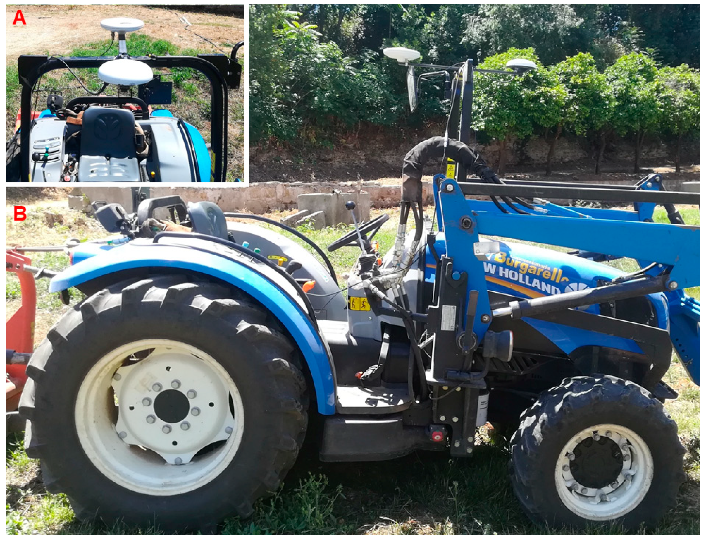
−1). The tests were carried out using a wheeled tractor owned by the University of Palermo (
Figure 2). The receivers were placed on the dashboard, while the external antenna was mounted in the upper part of the roll bar. The tractor forward speed was kept constant in all tests and equal to 0.94 m s
−1 during all tests.
Different tests were carried out in order to evaluate the positioning accuracy of the different GNSS receivers. The tests were distinguished by the use or not of RTK differential correction data and/or an external antenna. In fact, only the differential correction data transmitted in real-time from the network of RTK ground stations (CORS) were selected, as this technique allows for better accuracy [
23].
The accuracy of each GNSS receiver was evaluated by comparing the distance between the different positions logged by it during the different tests and those determined by means of the reference receiver, i.e., Stonex S7-G, used with external antenna and RTK differential correction. The longitude and latitude differences in UTM-WGS84 projection were computed. In order to evaluate the accuracy of the tested GNSS receivers, differential correction data were used: the satellite receivers were linked to the UNIPA GNSS CORS station located in the University of Palermo Campus (210 m from the geometric centre of the testing field) via NTRIP, having a frequency of 1 Hz (1 position s
−1) [
24].
A total of 10 tests named with the letters A, B, C, D, E, F, G, H, I, L, M were carried out using the four GNSS receivers described above, with and without RTK differential correction and/or with and without external antenna (
Table 1). Each dynamic test, carried out in RTK mode, was replicated three times in order to obtain significant results.
The satellite receivers S7 and S5 determined the geodetic coordinates of the points by using or not using RTK differential correction data (tests A–B and E–F) and the external and internal antenna (tests C-D and G-H). The receiver TMMP was tested only with and without the external antenna (tests I-L), as this instrument was not able to receive differential correction data in real time. Finally, the receiver QLV2 was tested only with the internal antenna (test M).
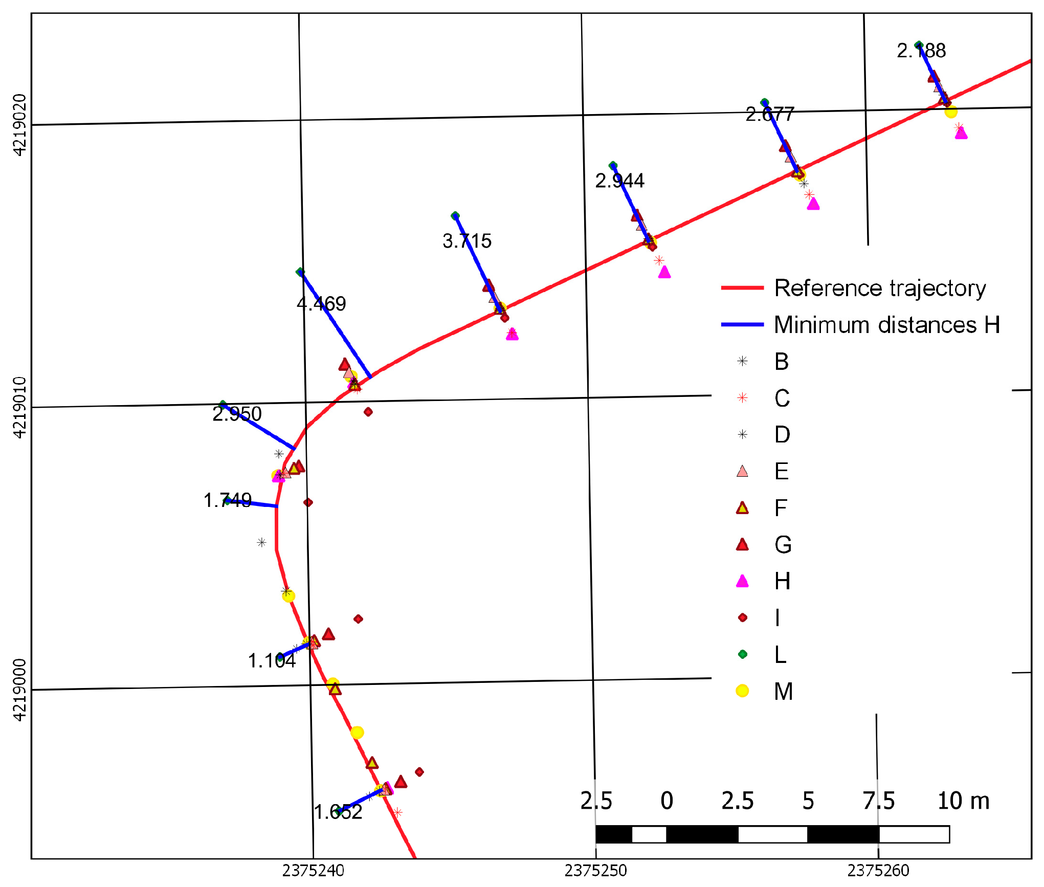
The geodetic coordinates of the points determined by the satellite receivers used in the different tests were processed by means of a GIS software. The points determined by each GNSS receiver under the different testing conditions were compared with the reference trajectory by means of QGIS software.
Fifty sample points were extracted from the trajectories drawn by joining the points determined by the receivers. Since the field perimeter was 287 m, these points were 5.74 m away from each other. The shortest distance from the sample points of every test to the reference track line was calculated in QGIS by means of “shortest_line” Geometry Function. This returns the shortest line joining two geometries. The shortest distance from a point to a line segment is the perpendicular to the line segment. If a perpendicular cannot be drawn within the end vertices of the line segment, then the distance to the nearest end vertex is the shortest distance (
Figure 3).
2.4. Statistical Analysis
The position data determined using the four satellite receivers in the different tests were subjected to analysis of variance (ANOVA) and Tukey’s test in order to evaluate the statistical significance of the tests at 95% confidence level [
25]. Principal Component Analysis (PCA) was applied in order to reduce the variable data setting and extract composite quality indicators. Each distance was considered as the dependent variable of the measured experimental parameters. The obtained principal components were considered as significant if their Eigen values were >1. All the statistical analyses were carried out using Statgraphics Centurion (Statpoint Inc., The Plains, VA, USA, 2005).
3. Results and Discussion
The trajectories obtained by using the tested GNSS receivers are shown together with the reference one, i.e., Stonex S7-G, in
Figure 4.
The summary statistics of the data are shown in
Table 2, while the results of the related Analysis of Variance is shown in
Table 3.
The S7 receiver, used in tests B, C and D, recorded an error with a larger relative dispersion in test C, i.e., without RTK differential correction and with external antenna, with a coefficient of variation equal to 63.62% and with a positioning error between 0.06 and 1.06 m. The S5 receiver, used in tests E, F, G and H, provided a positioning error with a larger relative dispersion in test E (coefficient of variation equal to 64.68%) and error values between 0 and 0.59 m. The receiver that showed the highest relative dispersion was the TMMP in test I with a coefficient of variation of 90.44% and error values between 0.03 and 1.77 m. The cheapest receiver, QLV2, used in test M, recorded a coefficient of variation equal to 69.59% and a positioning error ranging from 0 to 1.28 m. Test G, carried out by using the S5 receiver with external antenna without differential correction, provided the lowest relative dispersion, with a positioning error between 0.58 and 1.18 m.
The ANOVA table decomposes the variance of the data into two components: a between-group component and a within-group component. The F-ratio, which in this case equals 56.4953, is a ratio of the between-group estimate to the within-group estimate. Since the p-value of the F-test is lower than 0.05, there is a statistically significant difference between the means of the 11 variables at the 5% significance level.
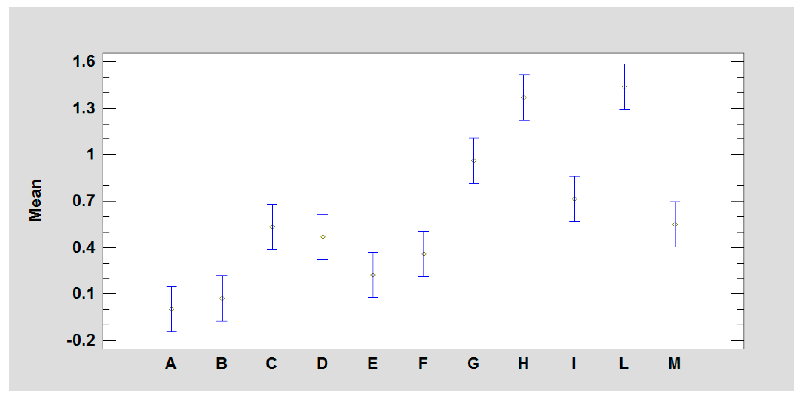
Table 4 shows the results of a multiple comparison procedure application able to determine which means are significantly different from which others. Seven homogenous groups were identified using columns of Xs. The levels containing Xs form a group of means within which there are no statistically significant differences. The method currently being used to discriminate among the means is Tukey’s Honestly Significant Difference (HSD) procedure. With this method, there is a 5.0% risk of calling one or more pairs significantly different when their actual difference equals 0 (
Figure 5).
Table 5 shows the estimated difference between each pair of means. An asterisk has been placed next to 38 pairs, indicating that these pairs show statistically significant differences at a 95.0% confidence level.
No statistically significant differences were obtained between the averages of the distances of tests A and B. Instead, statistically significant differences between tests A-C, A-D, B-C and B-D were noted. The highest differences were recorded between tests A-C, where test C obtained an average error of 0.532 m with respect to test A. From the comparison between the average errors recorded in tests C and D, carried out by using the S7 receiver in the modes with and without external antenna, there were no statistically significant differences.
With reference to the S5 receiver, no statistically significant differences were obtained between tests E and F. On the other hand, there were statistically significant differences between tests E-G, E-H, F-G, F-H and G-H. The highest differences were recorded between tests E-H with a difference of 1.148 m. Unlike the S7 receiver, the S5 showed statistically significant differences between tests G and H, respectively, with and without external antenna, with a positioning error in test H about 30% higher than G. These results highlight the importance of using the external antenna for improving the reception of satellite signals [
10,
11].
As regards the TMMP receiver, statistically significant differences were obtained between tests I and L, respectively, with and without external antenna. The average error ranged from 0.715 m with external antenna to 1.439 m without external antenna.
Finally, the low-cost receiver QLV2, used in test M without RTK differential correction and external antenna, provided an average error value of 0.550 m. If this receiver is compared to the others, tests A and B, performed with the S7 receiver, provided better positioning accuracy, while worse accuracy was obtained in test H performed with the S5 receiver (without RTK and external antenna) and in test L (also without RTK and external antenna) performed with the TMMP receiver. Instead, there were no statistically significant differences between the average positioning error of the QLV2 receiver and that of the S7 (used without differential correction both with and without external antenna in tests C and D), as well as between the QLV2 receiver and both the S5 (used with RTK differential correction and without external antenna in test F) and the TMMP (used in test I).
By comparing the receivers used in RTK mode (S7 and S5), i.e., tests A-E and B-F, no statistically significant differences were obtained.
The purpose of the PCA is to obtain a small number of linear combinations of the ten variables which account for most of the variability in the data. In this case, ten components were extracted. Together, they account for 100.0% of the variability in the original data.
Table 6 reports all the ten components extracted from PCA performed on the data. The first column lists the Eigen values of the correlation matrix, ordered from the highest to the lowest. As a correlation matrix was analysed, the variables were standardised to have unit variance, so the total variance was 10. As the Eigen values are the variances of the principal components, the first principal component had a variance of 4.0987, explaining 41% (4.0987/10) of the total variance; the second component had a variance of 2.9029, explaining the 29% of the total variance, and so on for the other components. Following the well-known and most-used Kaiser’s criterion [
26] and the scree plot (not shown in the paper) [
27], which suggest retaining components with Eigen values higher than 1, three components were extracted which explain 81% (41+29+11) of the total variance of the data components.
The factorability tests provide indications of whether or not it is likely to be worthwhile to attempt to extract factors from a set of variables. The Kaiser–Meyer–Olkin (KMO) statistic provides an indication of how much common variance is present. For factorisation to be worthwhile, KMO should normally be at least 0.6. Since KMO = 0.714463, factorisation is likely to provide interesting information about any underlying factor.
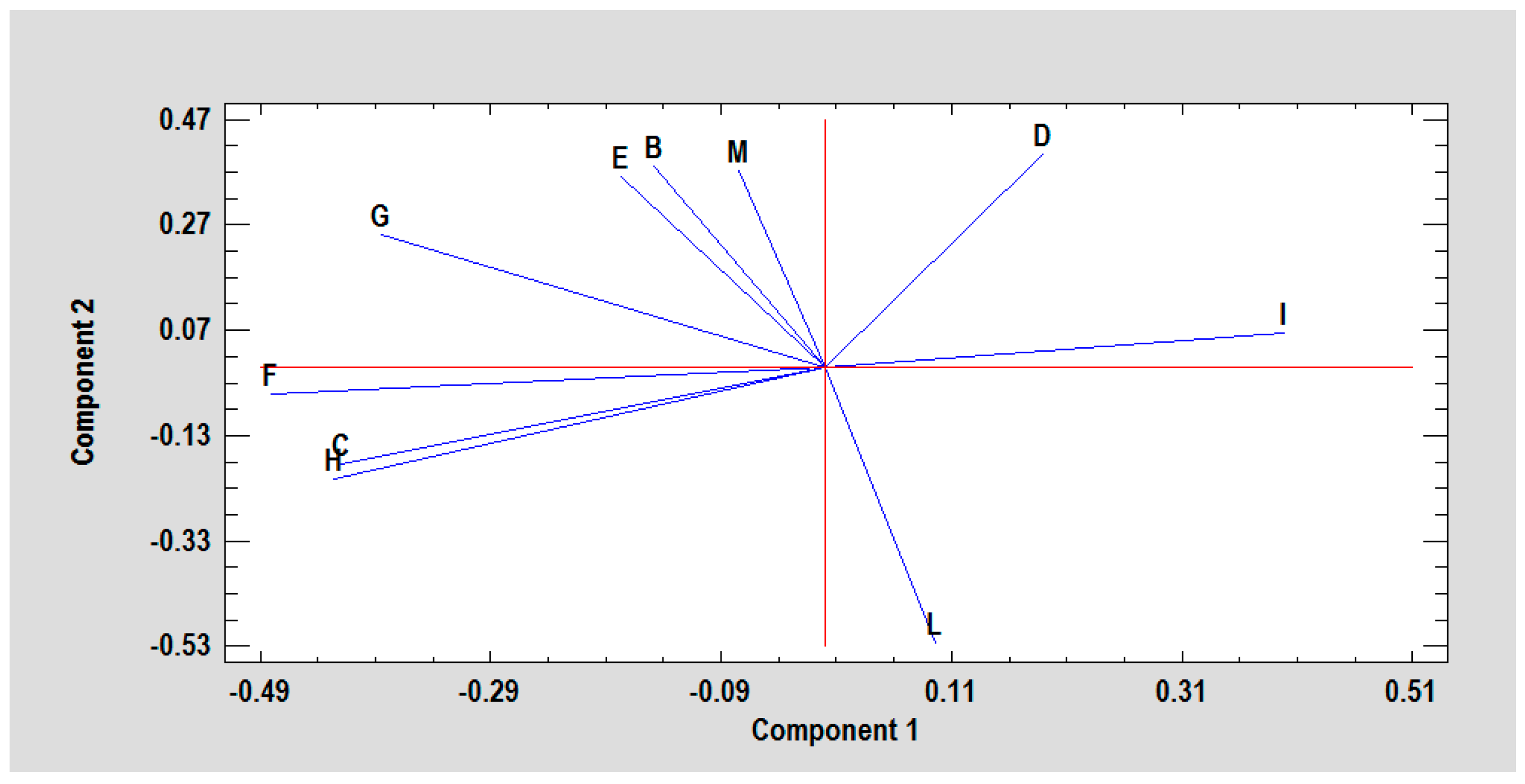
The score biplot (
Figure 6) gives us a feeling for the similarities and differences among the different tests. It shows that test L is opposite to B, E and M, while test I is opposite to C, F and H.
The results of the evaluation carried out by Jackson et al. [
7] with reference to the GNSS receiver Navcom SF-3050 showed that, generally, the low-cost receivers do not achieve the same positioning accuracy as the survey-grade ones. All low-cost single-frequency (L1) receivers evaluated by these authors, during static applications, could achieve centimetre-level accuracy in rural environments and perform better when using high quality versus a low-quality antenna. However, during dynamic applications, they could not determine an RTK position at any time. Among the low-cost L1 frequency receivers tested by the above authors, Reach showed a centimetre-level 95% accuracy. Among the tested L1/L2 frequency receivers, Piksi Multi showed a positioning accuracy of 0.048 m, while Eclipse P307 had an accuracy of 0.069 m [
7].
The results obtained during the performed tests are perfectly aligned with those achieved by Yuwono et al. [
10]: dual-frequency (L1/L2) GNSS receivers were better than single-frequency (L1) receivers.
In fact, a distance from the determined points to the reference trajectory (test A) up to 0.221 m was recorded in tests B and E. Therefore, the S7 and S5 receivers can be used in RTK mode on agricultural farms where row crops, e.g., tree and horticultural crops, are cultivated: these receivers allow the spatially variable rate application of crop inputs (e.g., fertilisers, herbicides, pesticides) by respecting the distance between the rows and without causing any damage to the crop. A distance from the determined points to the reference trajectory up to 0.532 m was recorded in tests F, D, C and M. Therefore, the S7 receiver, with or without external antenna and without differential correction, the S5 receiver, in RTK mode and without external antenna, and the low-cost QLV2 receiver can be used on all farms, for mapping crop yield, soil nutrients and humidity. A distance from the determined points to the reference trajectory up to 0.962 m was recorded in tests I and G. As a consequence, the TMMP and S5 receivers, with external antenna and without differential correction, can be used for topographic surveys of areas larger than 50 hectares in order to quantify the Utilised Agricultural Area (UAA) and farm uncultivated areas. Finally, distance from the determined points to the reference trajectory up to 1.439 m was recorded in tests H and L. Therefore, the S5 and TMMP receivers, with internal antenna and without differential correction, can be used only in aided guidance systems of agricultural machines, both for traceability of crop operations and operator safety, according to [
28]. Generally, the use of low-cost receivers such as TMMP and QLV2 can allow location of the work site and, then, ensure prompt rescue interventions for operator safety.


 ,
, 


