
Designing Bioinspired Composite Structures via Genetic Algorithm and Conditional Variational Autoencoder


Abstract
:
1. Introduction
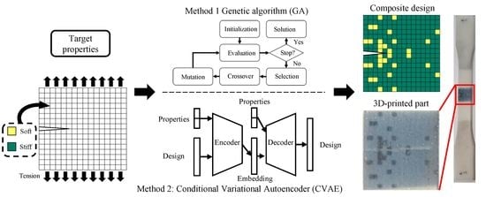
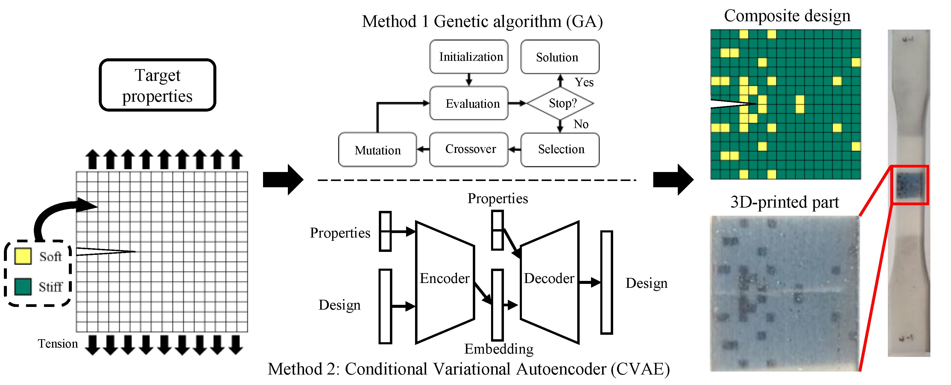
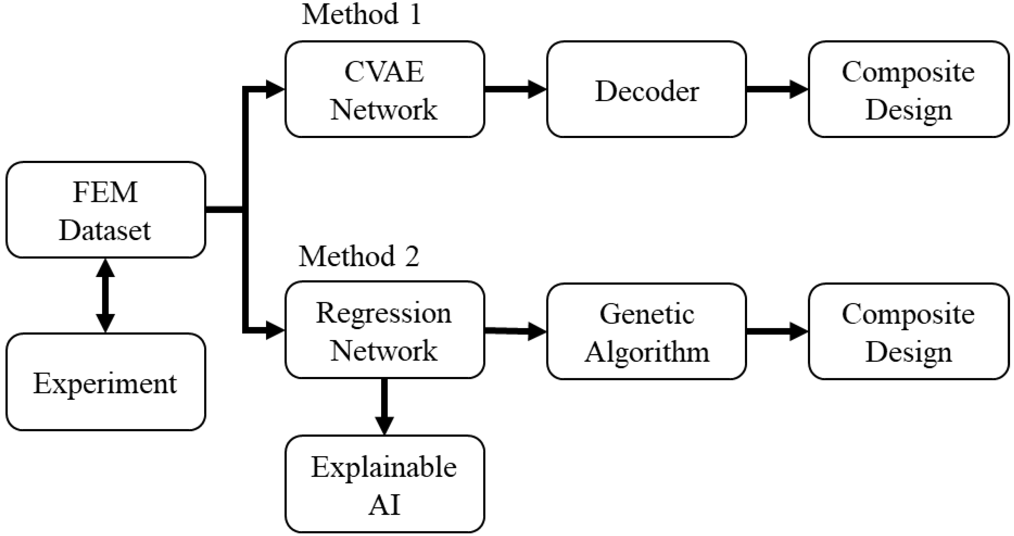
2. Materials and Methods
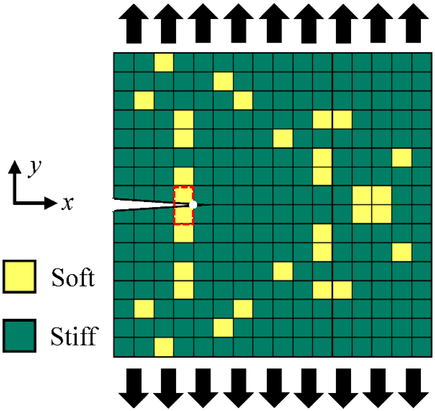
2.1. Composite Design Space, Fabrication, and Finite Element Analysis
2.2. Experimental Section

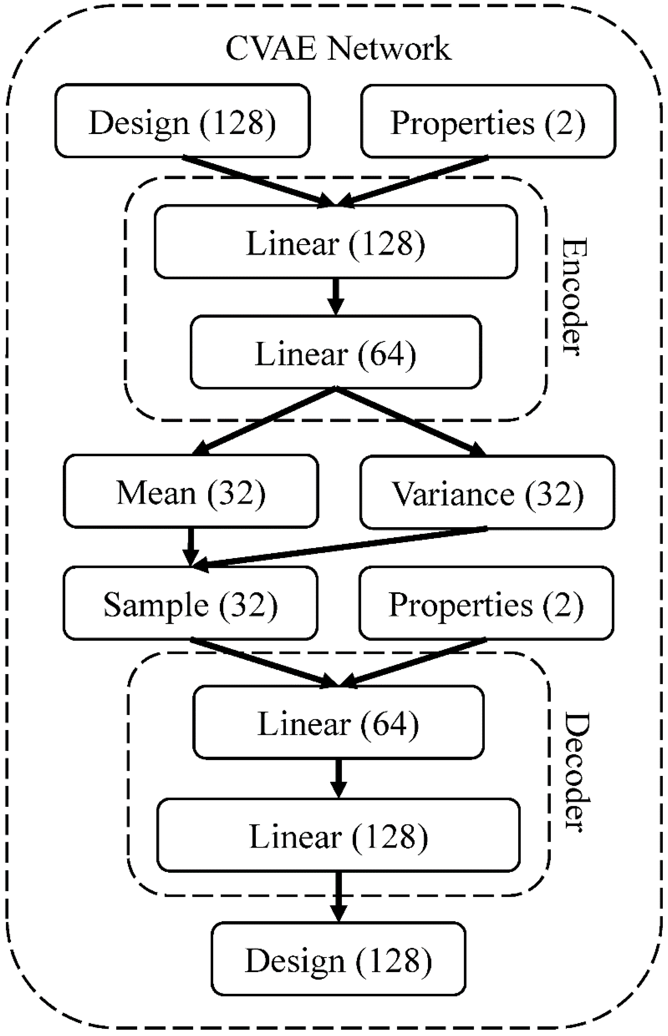
2.3. Conditional Variational Autoencoder (CVAE)
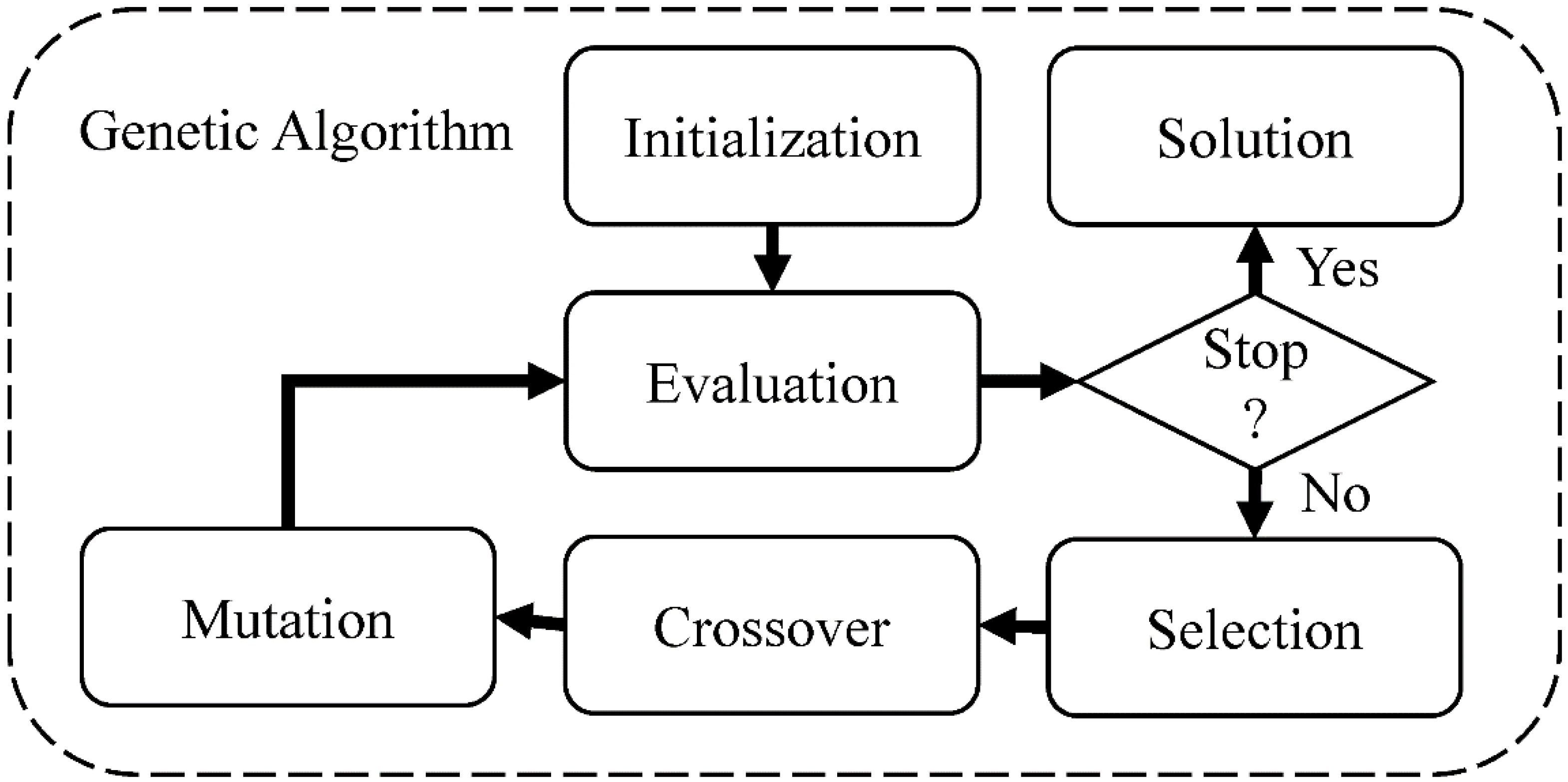
2.4. Genetic Algorithm (GA)
3. Results and Discussion
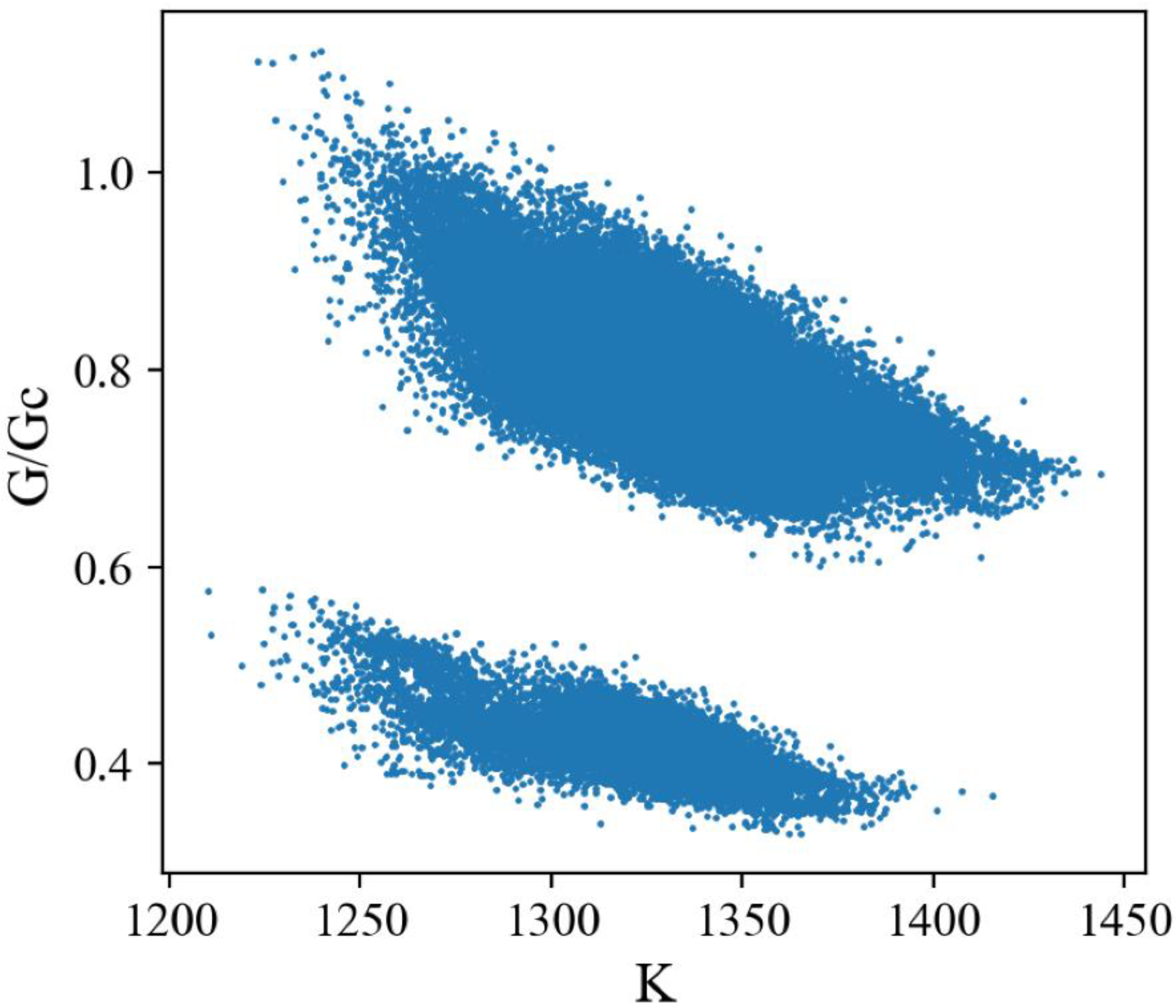
3.1. Dataset Analysis
3.2. Experimental Results
3.3. CVAE versus GA
3.4. Discussion with Explainable AI (XAI) and Fracture Mechanics
4. Conclusions
Author Contributions
Funding
Institutional Review Board Statement
Data Availability Statement
Conflicts of Interest
References
- Jackson, A.P.P.; Vincent, J.F.V.F.V.; Turner, R.M.M. The Mechanical Design of Nacre. Proc. R. Soc. B 1988, 234, 415–440. [Google Scholar] [CrossRef]
- Huss, J.C.; Antreich, S.J.; Bachmayr, J.; Xiao, N.; Eder, M.; Konnerth, J.; Gierlinger, N. Topological Interlocking and Geometric Stiffening as Complementary Strategies for Strong Plant Shells. Adv. Mater. 2020, 32, e2004519. [Google Scholar] [CrossRef] [PubMed]
- Chang, Y.; Chen, P.-Y.Y. Hierarchical Structure and Mechanical Properties of Snake (Naja Atra) and Turtle (Ocadia Sinensis) Eggshells. Acta Biomater. 2016, 31, 33–49. [Google Scholar] [CrossRef] [PubMed]
- Chiang, P.-L.; Tseng, Y.-C.; Wu, H.-J.; Tsao, S.-H.; Wu, S.-P.; Wang, W.-C.; Hsieh, H.-I.; Juang, J.-Y. Elastic Moduli of Avian Eggshell. Biology 2021, 10, 989. [Google Scholar] [CrossRef] [PubMed]
- Juang, J.Y.; Chen, P.Y.; Yang, D.C.; Wu, S.P.; Yen, A.; Hsieh, H.I. The Avian Egg Exhibits General Allometric Invariances in Mechanical Design. Sci. Rep. 2017, 7, 14205. [Google Scholar] [CrossRef] [PubMed] [Green Version]
- Huang, Y.-S.; Chiang, P.-L.; Kao, Y.-C.; Hsu, F.-L.; Juang, J.-Y. Cracking Failure of Curved Hollow Tree Trunks. R. Soc. Open Sci. 2020, 7, 200203. [Google Scholar] [CrossRef] [Green Version]
- Huang, Y.S.; Hsu, F.L.; Lee, C.M.; Juang, J.Y. Failure Mechanism of Hollow Tree Trunks Due to Cross-Sectional Flattening. R. Soc. Open Sci. 2017, 4, 160972. [Google Scholar] [CrossRef] [Green Version]
- Fratzl, P.; Weinkamer, R. Nature’s Hierarchical Materials. Prog. Mater Sci. 2007, 52, 1263–1334. [Google Scholar] [CrossRef] [Green Version]
- Munch, E.; Launey, M.E.; Alsem, D.H.; Saiz, E.; Tomsia, A.P.; Ritchie, R.O. Tough, Bio-Inspired Hybrid Materials. Science 2008, 322, 1516–1520. [Google Scholar] [CrossRef] [Green Version]
- Yin, Z.; Hannard, F.; Barthelat, F. Impact-Resistant Nacre-Like Transparent Materials. Science 2019, 364, 1260–1263. [Google Scholar] [CrossRef]
- Yu, C.-H.; Tseng, B.-Y.; Yang, Z.; Tung, C.-C.; Zhao, E.; Ren, Z.-F.; Yu, S.-S.; Chen, P.-Y.; Chen, C.-S.; Buehler, M.J. Hierarchical Multiresolution Design of Bioinspired Structural Composites Using Progressive Reinforcement Learning. Adv. Theory Simul. 2022, 5, 2200459. [Google Scholar] [CrossRef]
- Gu, G.X.; Chen, C.T.; Buehler, M.J. De Novo Composite Design Based on Machine Learning Algorithm. Extrem. Mech. Lett. 2018, 18, 19–28. [Google Scholar] [CrossRef]
- Libonati, F.; Gu, G.X.; Qin, Z.; Vergani, L.; Buehler, M.J. Bone-Inspired Materials by Design: Toughness Amplification Observed Using 3d Printing and Testing. Adv. Eng. Mater. 2016, 18, 1354–1363. [Google Scholar] [CrossRef] [Green Version]
- Chawla, K.K. Composite Materials: Science and Engineering, 3rd ed.; Springer Science+Business Media: New York, NY, USA, 2012; p. 542. [Google Scholar]
- Canale, G.; Andrews, S.; Rubino, F.; Maligno, A.; Citarella, R.; Weaver, P.M. Realistic Stacking Sequence Optimisation of an Aero-Engine Fan Blade-Like Structure Subjected to Frequency, Deformation and Manufacturing Constraints. Open Mech. Eng. J. 2018, 12, 151–163. [Google Scholar] [CrossRef]
- Herencia, J.E.; Weaver, P.M.; Friswell, M.I. Optimization of Long Anisotropic Laminated Fiber Composite Panels with T-Shaped Stiffeners. AIAA J. 2007, 45, 2497–2509. [Google Scholar] [CrossRef] [Green Version]
- Barbero, E.J. Introduction to Composite Materials Design, 3rd ed.; CRC Press, Taylor & Francis Group: Boca Raton, FL, USA, 2018; p. 535. [Google Scholar]
- Mallick, P.K. Fiber-Reinforced Composites: Materials, Manufacturing, and Design, 3rd ed.; CRC Press: Boca Raton, FL, USA, 2008; p. 619. [Google Scholar]
- Gibson, I.; Rosen, D.W.; Stucker, B. Additive Manufacturing Technologies: 3d Printing, Rapid Prototyping and Direct Digital Manufacturing, 2nd ed.; Springer: New York, NY, USA; London, UK, 2015; p. 498. [Google Scholar]
- Studart, A.R. Additive Manufacturing of Biologically-Inspired Materials. Chem. Soc. Rev. 2016, 45, 359–376. [Google Scholar] [CrossRef]
- Ghimire, A.; Tsai, Y.-Y.; Chen, P.-Y.; Chang, S.-W. Tunable Interface Hardening: Designing Tough Bio-Inspired Composites through 3d Printing, Testing, and Computational Validation. Compos. Part B Eng. 2021, 215, 108754. [Google Scholar] [CrossRef]
- Hajela, P.; Lee, E.; Lin, C.-Y. Genetic Algorithms in Structural Topology Optimization. In Topology Design of Structures; Springer: Berlin/Heidelberg, Germany, 1993; pp. 117–133. [Google Scholar]
- Hamel, C.M.; Roach, D.J.; Long, K.N.; Demoly, F.; Dunn, M.L.; Qi, H.J. Machine-Learning Based Design of Active Composite Structures for 4d Printing. Smart Mater. Struct. 2019, 28, 065005. [Google Scholar] [CrossRef]
- Yu, C.-H.; Qin, Z.; Buehler, M.J. Artificial Intelligence Design Algorithm for Nanocomposites Optimized for Shear Crack Resistance. Nano Futures 2019, 3, 035001. [Google Scholar] [CrossRef]
- Gu, G.X.; Dimas, L.; Qin, Z.; Buehler, M.J. Optimization of Composite Fracture Properties: Method, Validation, and Applications. J. Appl. Mech. 2016, 83, 071006. [Google Scholar] [CrossRef]
- Holland, J.H. Genetic Algorithm. Sci. Am. 1992, 267, 66–72. [Google Scholar] [CrossRef]
- Mathias, J.-D.; Balandraud, X.; Grediac, M. Applying a Genetic Algorithm to the Optimization of Composite Patches. Comput. Struct. 2006, 84, 823–834. [Google Scholar] [CrossRef]
- Soremekun, G.; Gürdal, Z.; Haftka, R.T.; Watson, L.T. Composite Laminate Design Optimization by Genetic Algorithm with Generalized Elitist Selection. Comput. Struct. 2001, 79, 131–143. [Google Scholar] [CrossRef]
- Jenkins, W.M. Towards Structural Optimization Via the Genetic Algorithm. Comput. Struct. 1991, 40, 1321–1327. [Google Scholar] [CrossRef]
- Tromp, J. The Number of Legal Go Positions. In Proceedings of International Conference on Computers and Games; Springer: Cham, Switzerland, 2016; pp. 183–190. [Google Scholar]
- Silver, D.; Huang, A.; Maddison, C.J.; Guez, A.; Sifre, L.; van den Driessche, G.; Schrittwieser, J.; Antonoglou, I.; Panneershelvam, V.; Lanctot, M.; et al. Mastering the Game of Go with Deep Neural Networks and Tree Search. Nature 2016, 529, 484–489. [Google Scholar] [CrossRef]
- Pilania, G.; Wang, C.; Jiang, X.; Rajasekaran, S.; Ramprasad, R. Accelerating Materials Property Predictions Using Machine Learning. Sci. Rep. 2013, 3, 2810. [Google Scholar] [CrossRef] [Green Version]
- Ahneman, D.T.; Estrada, J.G.; Lin, S.; Dreher, S.D.; Doyle, A.G. Predicting Reaction Performance in C-N Cross-Coupling Using Machine Learning. Science 2018, 360, 186–190. [Google Scholar] [CrossRef] [Green Version]
- Chen, C.-T.; Gu, G.X. Machine Learning for Composite Materials. MRS Commun. 2019, 9, 556–566. [Google Scholar] [CrossRef] [Green Version]
- Ye, S.; Li, B.; Li, Q.; Zhao, H.-P.; Feng, X.-Q. Deep Neural Network Method for Predicting the Mechanical Properties of Composites. Appl. Phys. Lett. 2019, 115, 161901. [Google Scholar] [CrossRef]
- Daghigh, V.; Lacy, T.E., Jr.; Daghigh, H.; Gu, G.; Baghaei, K.T.; Horstemeyer, M.F.; Pittman, C.U., Jr. Machine Learning Predictions on Fracture Toughness of Multiscale Bio-Nano-Composites. J. Reinf. Plast. Compos. 2020, 39, 587–598. [Google Scholar] [CrossRef]
- Yang, Z.; Yu, C.-H.; Buehler, M.J. Deep Learning Model to Predict Complex Stress and Strain Fields in Hierarchical Composites. Sci. Adv. 2021, 7, eabd7416. [Google Scholar] [CrossRef]
- Yang, C.; Kim, Y.; Ryu, S.; Gu, G.X. Prediction of Composite Microstructure Stress-Strain Curves Using Convolutional Neural Networks. Mater. Des. 2020, 189, 108509. [Google Scholar] [CrossRef]
- Chang, H.-S.; Huang, J.-H.; Tsai, J.-L. Predicting Mechanical Properties of Unidirectional Composites Using Machine Learning. Multiscale Sci. Eng. 2022, 4, 202–210. [Google Scholar] [CrossRef]
- Tan, R.K.; Zhang, N.L.; Ye, W. A Deep Learning–Based Method for the Design of Microstructural Materials. Struct. Multidiscip. Optim. 2020, 61, 1417–1438. [Google Scholar] [CrossRef]
- Kim, B.; Lee, S.; Kim, J. Inverse Design of Porous Materials Using Artificial Neural Networks. Sci. Adv. 2020, 6, eaax9324. [Google Scholar] [CrossRef] [Green Version]
- Ni, B.; Gao, H. A Deep Learning Approach to the Inverse Problem of Modulus Identification in Elasticity. MRS Bull. 2020, 46, 19–25. [Google Scholar] [CrossRef]
- Lim, J.; Ryu, S.; Kim, J.W.; Kim, W.Y. Molecular Generative Model Based on Conditional Variational Autoencoder for De Novo Molecular Design. J. Cheminf. 2018, 10, 31. [Google Scholar] [CrossRef] [Green Version]
- Kang, S.; Cho, K. Conditional Molecular Design with Deep Generative Models. J. Chem Inf. Model. 2019, 59, 43–52. [Google Scholar] [CrossRef] [Green Version]
- Skalic, M.; Jiménez, J.; Sabbadin, D.; De Fabritiis, G. Shape-Based Generative Modeling for De Novo Drug Design. J. Chem Inf. Model. 2019, 59, 1205–1214. [Google Scholar] [CrossRef]
- Shrikumar, A.; Greenside, P.; Kundaje, A. Learning Important Features through Propagating Activation Differences. In Proceedings of Proceedings of the 34th International Conference on Machine Learning, Proceedings of Machine Learning Research, Sydney, Australia, 6–11 August 2017; pp. 3145–3153. [Google Scholar]
- Ribeiro, M.T.; Singh, S.; Guestrin, C. “Why Should I Trust You?” Explaining the Predictions of Any Classifier. In Proceedings of the 22nd ACM SIGKDD International Conference on Knowledge Discovery and Data Mining, San Francisco, CA, USA, 13–17 August 2016; pp. 1135–1144. [Google Scholar]
- Datta, A.; Sen, S.; Zick, Y. Algorithmic Transparency Via Quantitative Input Influence: Theory and Experiments with Learning Systems. In Proceedings of the 2016 IEEE Symposium on Security and Privacy (SP), San Jose, CA, USA, 22–26 May 2016; pp. 598–617. [Google Scholar]
- Bach, S.; Binder, A.; Montavon, G.; Klauschen, F.; Müller, K.-R.; Samek, W. On Pixel-Wise Explanations for Non-Linear Classifier Decisions by Layer-Wise Relevance Propagation. PLoS One 2015, 10, e0130140. [Google Scholar] [CrossRef]
- Lundberg, S.M.; Lee, S.-I. A Unified Approach to Interpreting Model Predictions. In Proceedings of the 31st International Conference on Neural Information Processing Systems, Long Beach, CA, USA, 4–9 December 2017; pp. 4768–4777. [Google Scholar]
- Anderson, T.L. Fracture Mechanics: Fundamentals and Applications, 4th ed.; CRC Press/Taylor & Francis: Boca Raton, FL, USA, 2017; p. 661. [Google Scholar]
- Rohrer, B. How Do Convolutional Neural Networks Work? Available online: https://e2eml.school/how_convolutional_neural_networks_work.html (accessed on 15 December 2022).
- Lee, S.; Pharr, M. Sideways and Stable Crack Propagation in a Silicone Elastomer. Proc. Natl. Acad. Sci. USA 2019, 116, 201820424. [Google Scholar] [CrossRef] [PubMed] [Green Version]
- Park, S.-J.; Seo, M.-K. Chapter 4—Solid-Solid Interfaces. In Interface Science and Technology; Park, S.-J., Seo, M.-K., Eds.; Elsevier: Amsterdam, The Netherlands, 2011; Volume 18, pp. 253–331. [Google Scholar]
- Andreu, A.; Su, P.-C.; Kim, J.-H.; Ng, C.S.; Kim, S.; Kim, I.; Lee, J.; Noh, J.; Subramanian, A.S.; Yoon, Y.-J. 4d Printing Materials for Vat Photopolymerization. Addit. Manuf. 2021, 44, 102024. [Google Scholar] [CrossRef]
- Lopes, L.R.; Silva, A.F.; Carneiro, O.S. Multi-Material 3d Printing: The Relevance of Materials Affinity on the Boundary Interface Performance. Addit. Manuf. 2018, 23, 45–52. [Google Scholar] [CrossRef]
- Xu, Y.-X.; Juang, J.-Y. Measurement of Nonlinear Poisson’s Ratio of Thermoplastic Polyurethanes under Cyclic Softening Using 2d Digital Image Correlation. Polymers 2021, 13, 1498. [Google Scholar] [CrossRef] [PubMed]
- Blaber, J.; Adair, B.; Antoniou, A. Ncorr: Open-Source 2d Digital Image Correlation Matlab Software. Exp. Mech. 2015, 55, 1105–1122. [Google Scholar] [CrossRef]
- Kullback, S.; Leibler, R.A. On Information and Sufficiency. Ann. Math. Stat. 1951, 22, 79–86. [Google Scholar] [CrossRef]


| K (N/m) | G/Gc | G (J/m2) | |
|---|---|---|---|
| mean | 1337 | 0.735229 | 199.377518 |
| std | 25.40 | 0.130645 | 59.964850 |
| min | 1210 | 0.329780 | 82.115000 |
| 25% | 1324 | 0.728642 | 181.958000 |
| 50% | 1340 | 0.763818 | 190.629000 |
| 75% | 1353 | 0.804388 | 202.360000 |
| max | 1444 | 1.122954 | 464.903000 |
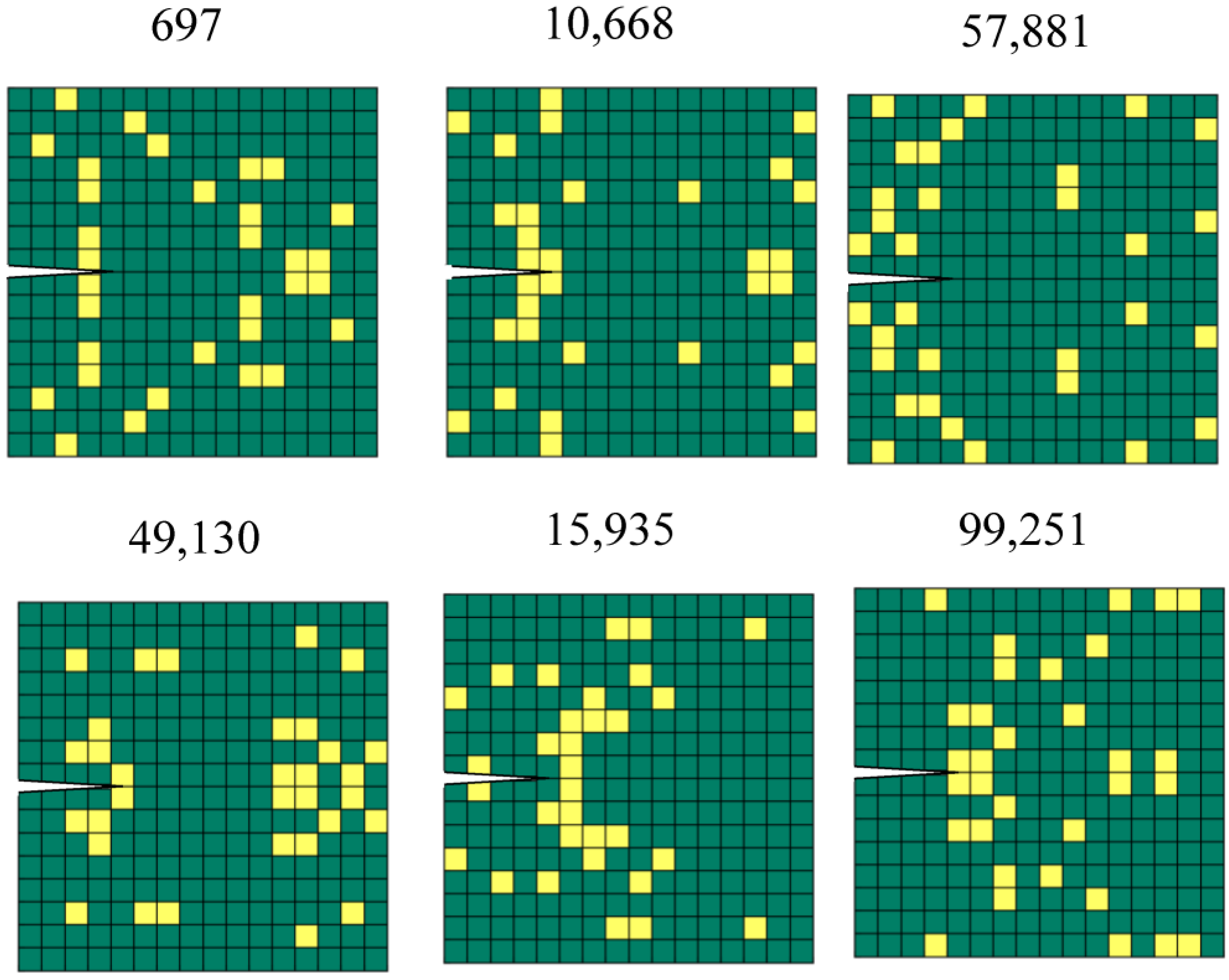
| No. | K (FEM) (N/m) | Experimental Stiffness, K (N/m) | Error (%) | |||
|---|---|---|---|---|---|---|
| Specimen 1 | Specimen 2 | Specimen 3 | Average | |||
| 697 | 1329 | 1478 | 1610 | 1396 | 1495 | 11.1 |
| 10,668 * | 1301 | 1546 | 1555 | 1424 | 1508 | 13.7 |
| 57,881 | 1375 | 1602 | 1423 | 1440 | 1488 | 8.6 |
| 49,130 * | 1308 | 1317 | 1365 | 1431 | 1371 | 4.6 |
| 15,935 | 1277 | 1478 | 1524 | 1362 | 1455 | 12.2 |
| 99,251 * | 1248 | 1347 | 1457 | 1324 | 1376 | 9.3 |
| No. | G/Gc | Experimental Toughness, (J/m3) | |||
|---|---|---|---|---|---|
| Specimen 1 | Specimen 2 | Specimen 3 | Average | ||
| 697 | 0.373 | 15,381 | 18,899 | 13,000 | 15,760 |
| 10,668 * | 0.374 | 15,114 | 9949 | 11,355 | 12,139 |
| 57,881 | 0.695 | 7971 | 9982 | 7836 | 8596 |
| 49,130 * | 0.693 | 9489 | 8141 | 8164 | 8598 |
| 15,935 | 1.008 | 9398 | 5734 | 5377 | 6836 |
| 99,251 * | 1.007 | 6698 | 6543 | 5819 | 6353 |
Disclaimer/Publisher’s Note: The statements, opinions and data contained in all publications are solely those of the individual author(s) and contributor(s) and not of MDPI and/or the editor(s). MDPI and/or the editor(s) disclaim responsibility for any injury to people or property resulting from any ideas, methods, instructions or products referred to in the content. |
© 2023 by the authors. Licensee MDPI, Basel, Switzerland. This article is an open access article distributed under the terms and conditions of the Creative Commons Attribution (CC BY) license (https://creativecommons.org/licenses/by/4.0/).
Share and Cite
Chiu, Y.-H.; Liao, Y.-H.; Juang, J.-Y. Designing Bioinspired Composite Structures via Genetic Algorithm and Conditional Variational Autoencoder. Polymers 2023, 15, 281. https://doi.org/10.3390/polym15020281
Chiu Y-H, Liao Y-H, Juang J-Y. Designing Bioinspired Composite Structures via Genetic Algorithm and Conditional Variational Autoencoder. Polymers. 2023; 15(2):281. https://doi.org/10.3390/polym15020281
Chicago/Turabian StyleChiu, Yi-Hung, Ya-Hsuan Liao, and Jia-Yang Juang. 2023. "Designing Bioinspired Composite Structures via Genetic Algorithm and Conditional Variational Autoencoder" Polymers 15, no. 2: 281. https://doi.org/10.3390/polym15020281