
Predicting Characteristics of Dissimilar Laser Welded Polymeric Joints Using a Multi-Layer Perceptrons Model Coupled with Archimedes Optimizer


Abstract
:1. Introduction
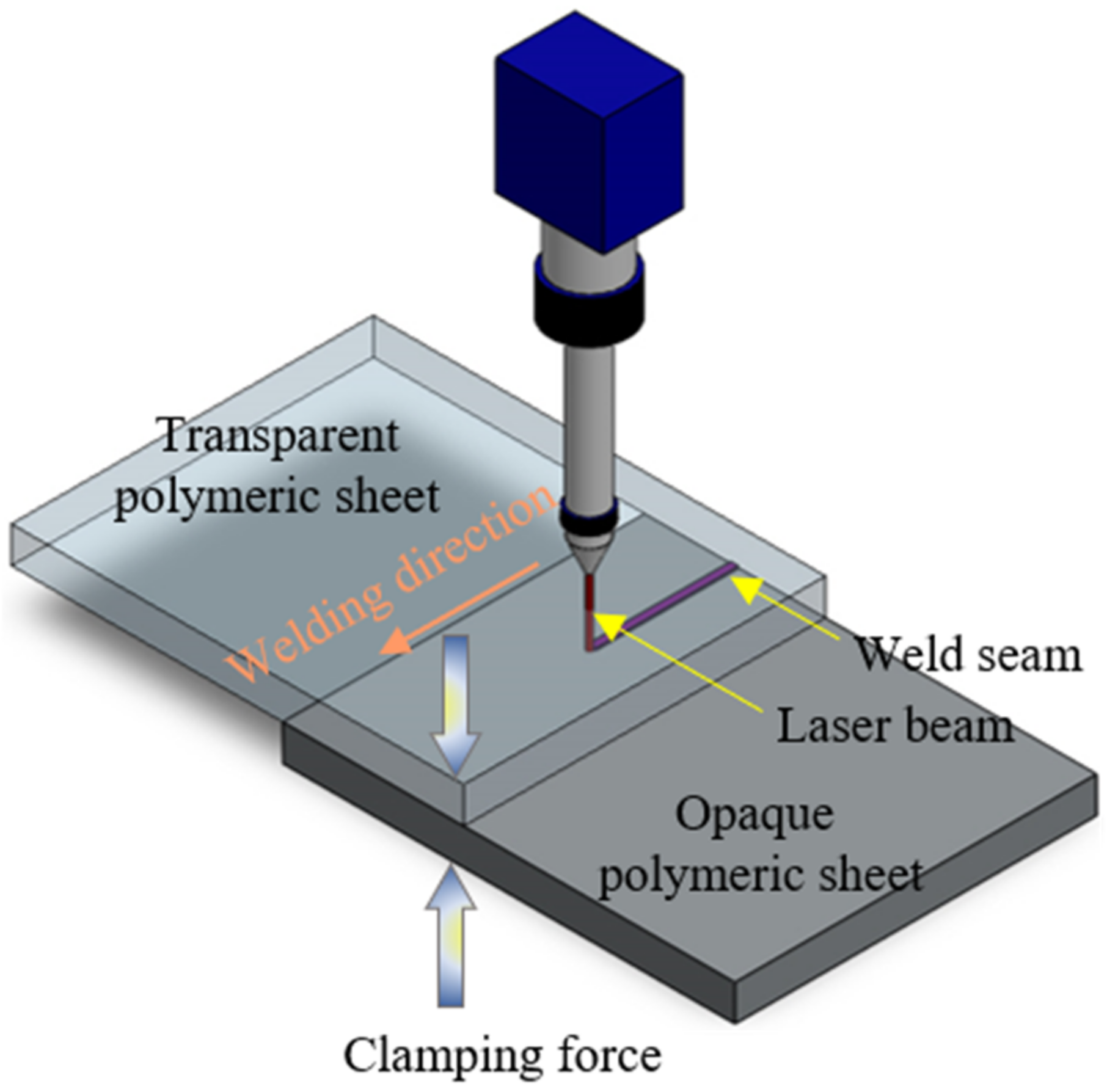
2. Experimentation
3. Modeling Approach
3.1. Multilayer Perceptron (MLP)
3.2. Archimedes Optimizer
3.3. Optimized Model
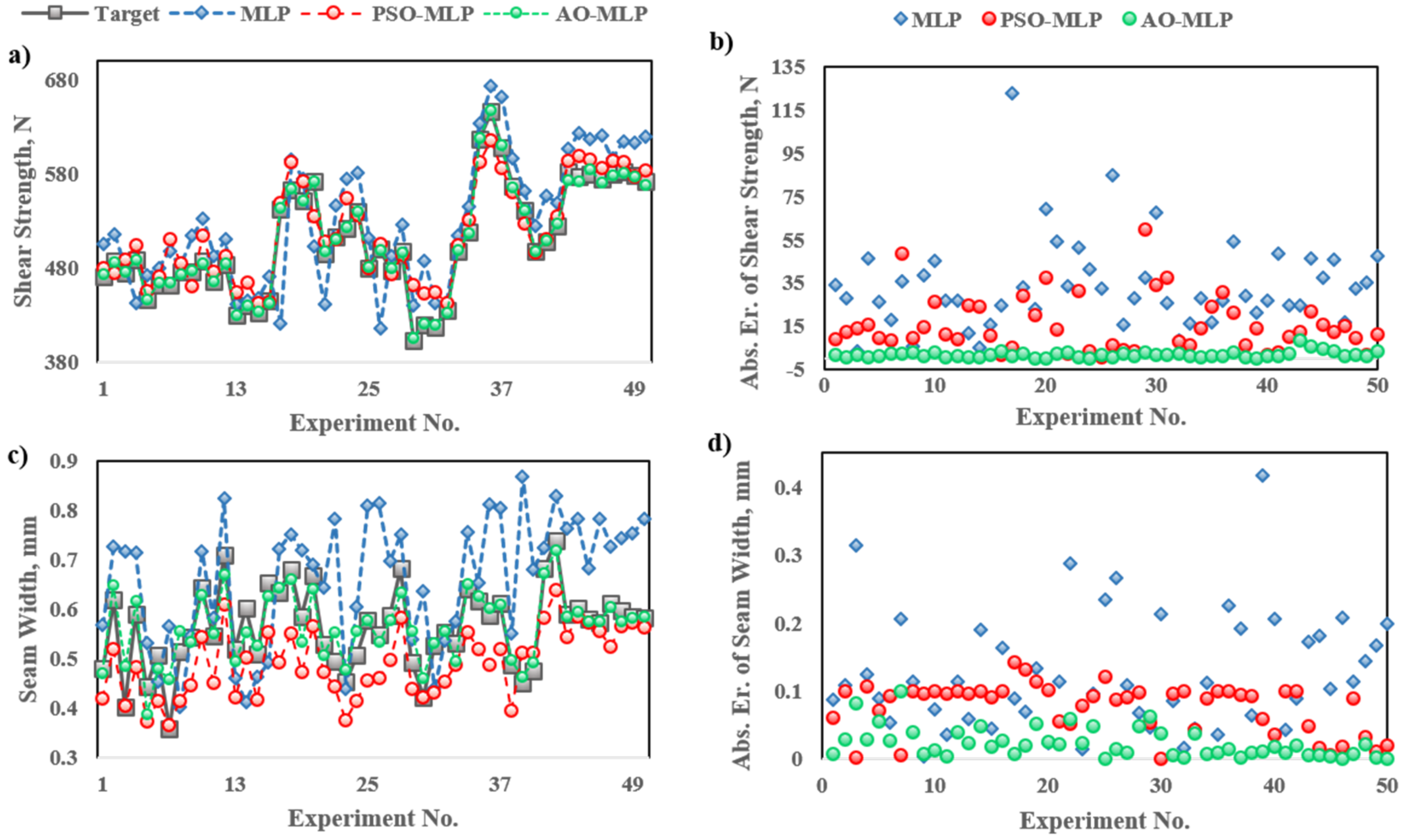
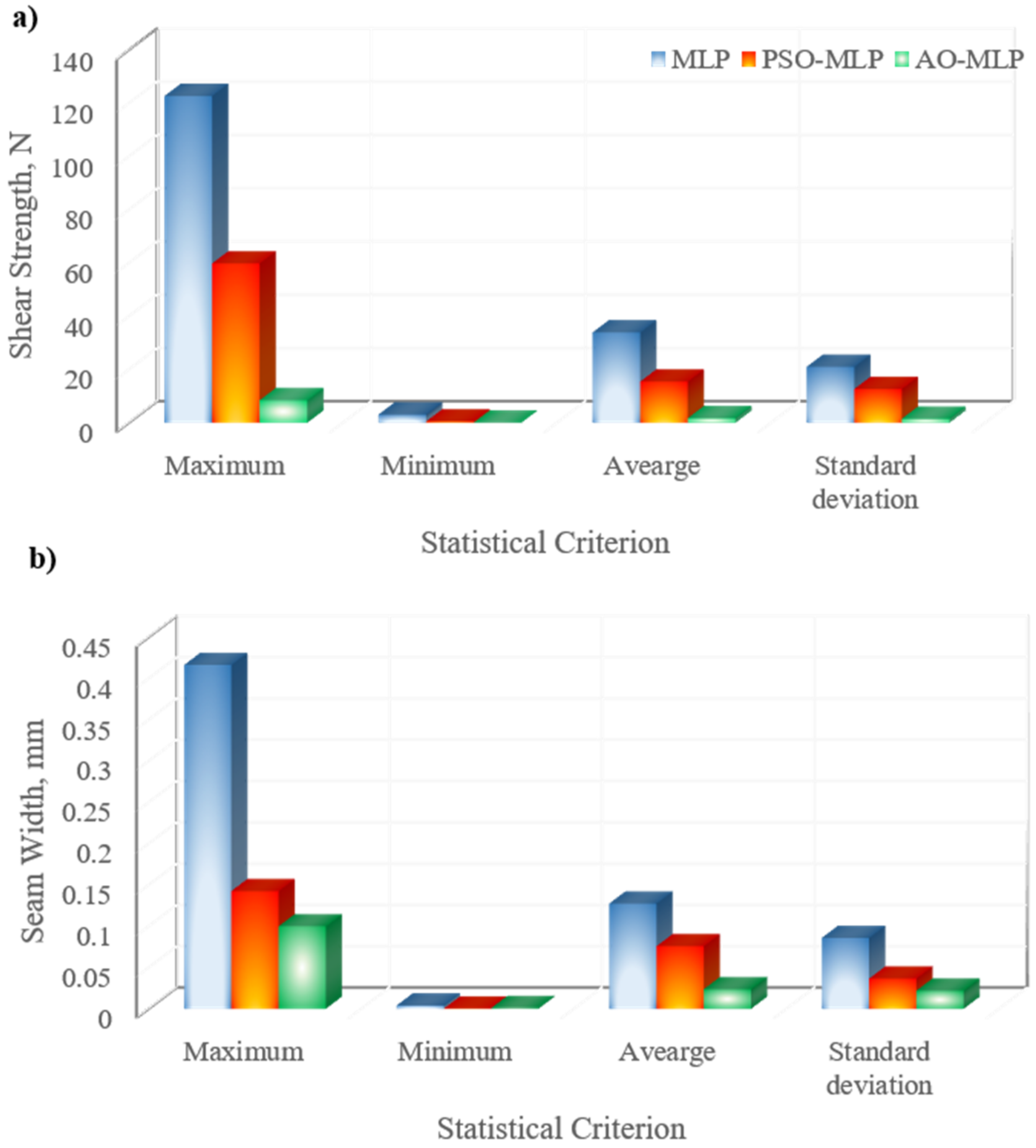
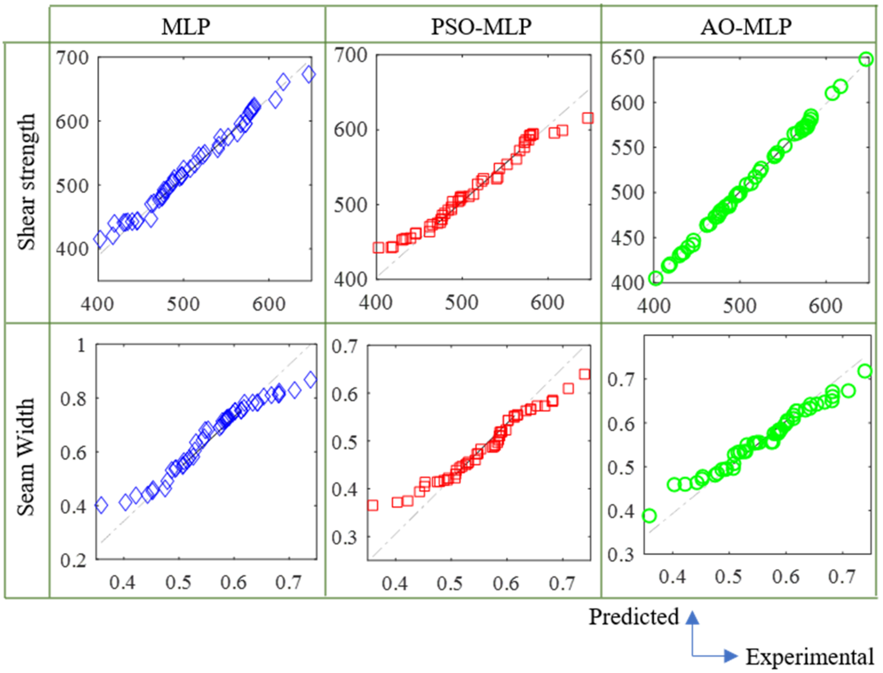
4. Results and Discussions
5. Conclusions
Author Contributions
Funding
Acknowledgments
Conflicts of Interest
References
- Ramanaviciene, A.; Plikusiene, I. Polymers in Sensor and Biosensor Design. Polymers 2021, 13, 917. [Google Scholar] [CrossRef] [PubMed]
- Abu-Okail, M.; Alsaleh, N.A.; Farouk, W.; Elsheikh, A.; Abu-Oqail, A.; Abdelraouf, Y.A.; Ghafaar, M.A. Effect of dispersion of alumina nanoparticles and graphene nanoplatelets on microstructural and mechanical characteristics of hybrid carbon/glass fibers reinforced polymer composite. J. Mater. Res. Technol. 2021, 14, 2624–2637. [Google Scholar] [CrossRef]
- Xu, Y.; Niu, Q.; Zhang, L.; Yuan, C.; Ma, Y.; Hua, W.; Zeng, W.; Min, Y.; Huang, J.; Xia, R. Highly Efficient Perovskite Solar Cell Based on PVK Hole Transport Layer. Polymers 2022, 14, 2249. [Google Scholar] [CrossRef] [PubMed]
- Zhang, Z.; Bellisario, D.; Quadrini, F.; Jestin, S.; Ravanelli, F.; Castello, M.; Li, X.; Dong, H. Nanoindentation of Multifunctional Smart Composites. Polymers 2022, 14, 2945. [Google Scholar] [CrossRef] [PubMed]
- Elsheikh, A. Bistable Morphing Composites for Energy-Harvesting Applications. Polymers 2022, 14, 1893. [Google Scholar] [CrossRef]
- Pereira, M.; Amaro, A.; Reis, P.; Loureiro, A. Effect of Friction Stir Welding Techniques and Parameters on Polymers Joint Efficiency—A Critical Review. Polymers 2021, 13, 2056. [Google Scholar] [CrossRef]
- Iftikhar, S.; Mourad, A.-H.; Sheikh-Ahmad, J.; Almaskari, F.; Vincent, S. A Comprehensive Review on Optimal Welding Conditions for Friction Stir Welding of Thermoplastic Polymers and Their Composites. Polymers 2021, 13, 1208. [Google Scholar] [CrossRef]
- Lai, H.; Fan, D.; Liu, K. The Effect of Welding Defects on the Long-Term Performance of HDPE Pipes. Polymers 2022, 14, 3936. [Google Scholar] [CrossRef]
- Amanat, N.; James, N.L.; McKenzie, D.R. Welding methods for joining thermoplastic polymers for the hermetic enclosure of medical devices. Med. Eng. Phys. 2010, 32, 690–699. [Google Scholar] [CrossRef]
- Zhao, P.; Tian, L.; Cui, X.; Xiong, X.; Wang, D.; Li, G. Hot gas implant welding of polypropylene via a three-dimensional porous copper implant. Compos. Commun. 2021, 25, 100761. [Google Scholar] [CrossRef]
- Bialaschik, M.; Schöppner, V.; Albrecht, M.; Gehde, M. Influence of material degradation on weld seam quality in hot gas butt welding of polyamides. Weld. World 2021, 65, 1161–1169. [Google Scholar] [CrossRef]
- Omer, M.A.E.; Rashad, M.; Elsheikh, A.H.; Showaib, E.A. A review on friction stir welding of thermoplastic materials: Recent advances and progress. Weld. World 2022, 66, 1–25. [Google Scholar] [CrossRef]
- Kuo, C.-C.; Xu, J.-Y.; Lee, C.-H. Weld Strength of Friction Welding of Dissimilar Polymer Rods Fabricated by Fused Deposition Modeling. Polymers 2022, 14, 2582. [Google Scholar] [CrossRef]
- Khalil, C.; Marya, S.; Racineux, G. Magnetic Pulse Welding and Spot Welding with Improved Coil Efficiency—Application for Dissimilar Welding of Automotive Metal Alloys. J. Manuf. Mater. Process. 2020, 4, 69. [Google Scholar] [CrossRef]
- Showaib, E.A.; Elsheikh, A.H. Effect of surface preparation on the strength of vibration welded butt joint made from PBT composite. Polym. Test. 2020, 83, 106319. [Google Scholar] [CrossRef]
- Qiu, J.; Zhang, G.; Sakai, E.; Liu, W.; Zang, L. Thermal Welding by the Third Phase Between Polymers: A Review for Ultrasonic Weld Technology Developments. Polymers 2020, 12, 759. [Google Scholar] [CrossRef] [Green Version]
- Kuo, C.-C.; Tsai, Q.-Z.; Li, D.-Y.; Lin, Y.-X.; Chen, W.-X. Optimization of Ultrasonic Welding Process Parameters to Enhance Weld Strength of 3C Power Cases Using a Design of Experiments Approach. Polymers 2022, 14, 2388. [Google Scholar] [CrossRef]
- Dave, F.; Ali, M.; Sherlock, R.; Kandasami, A.; Tormey, D. Laser Transmission Welding of Semi-Crystalline Polymers and Their Composites: A Critical Review. Polymers 2021, 13, 675. [Google Scholar] [CrossRef]
- Fernandes, F.A.; Pereira, A.B.; Guimarães, B.; Almeida, T. Laser Welding of Transmitting High-Performance Engineering Thermoplastics. Polymers 2020, 12, 402. [Google Scholar] [CrossRef] [Green Version]
- Gonçalves, L.F.; Duarte, F.M.; Martins, C.I.; Paiva, M.C. Laser welding of thermoplastics: An overview on lasers, materials, processes and quality. Infrared Phys. Technol. 2021, 119, 103931. [Google Scholar] [CrossRef]
- Acherjee, B. Laser transmission welding of polymers—A review on welding parameters, quality attributes, process monitoring, and applications. J. Manuf. Process. 2021, 64, 421–443. [Google Scholar] [CrossRef]
- Acherjee, B.; Kuar, A.S.; Mitra, S.; Misra, D. Laser transmission welding of polycarbonates: Experiments, modeling, and sensitivity analysis. Int. J. Adv. Manuf. Technol. 2014, 78, 853–861. [Google Scholar] [CrossRef]
- Acherjee, B. Laser transmission welding of polymers—A review on process fundamentals, material attributes, weldability, and welding techniques. J. Manuf. Process. 2020, 60, 227–246. [Google Scholar] [CrossRef]
- Nguyen, N.-P.; Behrens, S.; Brosda, M.; Olowinsky, A.; Gillner, A. Laser transmission welding of absorber-free semi-crystalline polypropylene by using a quasi-simultaneous irradiation strategy. Weld. World 2020, 64, 1227–1235. [Google Scholar] [CrossRef]
- Chen, Z.; Zhou, H.; Wu, C.; Han, F.; Yan, H. A cleaner production method for laser transmission welding of two transparent PMMA parts using multi-core copper wire. J. Mater. Res. Technol. 2022, 16, 1–12. [Google Scholar] [CrossRef]
- Wang, C.; Yu, X.; Wang, C.; Liu, Y.; Xia, Z. Laser transmission welding of Polyarylsulfone using zinc particles absorber. Infrared Phys. Technol. 2021, 118, 103892. [Google Scholar] [CrossRef]
- Jankus, S.M.; Bendikiene, R. Effect of the meltdown on thermoplastic joint produced by quasi-simultaneous laser transmission welding. CIRP J. Manuf. Sci. Technol. 2022, 39, 104–114. [Google Scholar] [CrossRef]
- Yu, X.; Long, Q.; Chen, Y.; Liu, Y.; Yang, C.; Jia, Q.; Wang, C. Laser transmission welding of dissimilar transparent thermoplastics using different metal particle absorbents. Opt. Laser Technol. 2022, 150, 108005. [Google Scholar] [CrossRef]
- Acherjee, B. Laser transmission welding of dissimilar plastics: 3-D FE modeling and experimental validation. Weld. World 2021, 65, 1429–1440. [Google Scholar] [CrossRef]
- Elsheikh, A.H.; Elaziz, M.A.; Das, S.R.; Muthuramalingam, T.; Lu, S. A new optimized predictive model based on political optimizer for eco-friendly MQL-turning of AISI 4340 alloy with nano-lubricants. J. Manuf. Process. 2021, 67, 562–578. [Google Scholar] [CrossRef]
- Elsheikh, A.H.; Panchal, H.; Ahmadein, M.; Mosleh, A.O.; Sadasivuni, K.K.; Alsaleh, N.A. Productivity forecasting of solar distiller integrated with evacuated tubes and external condenser using artificial intelligence model and moth-flame optimizer. Case Stud. Therm. Eng. 2021, 28, 101671. [Google Scholar] [CrossRef]
- Zayed, M.E.; Zhao, J.; Li, W.; Elsheikh, A.H.; Elaziz, M.A.; Yousri, D.; Zhong, S.; Mingxi, Z. Predicting the performance of solar dish Stirling power plant using a hybrid random vector functional link/chimp optimization model. Sol. Energy 2021, 222, 1–17. [Google Scholar] [CrossRef]
- Khoshaim, A.B.; Moustafa, E.B.; Bafakeeh, O.T.; Elsheikh, A.H. An Optimized Multilayer Perceptrons Model Using Grey Wolf Optimizer to Predict Mechanical and Microstructural Properties of Friction Stir Processed Aluminum Alloy Reinforced by Nanoparticles. Coatings 2021, 11, 1476. [Google Scholar] [CrossRef]
- Elmaadawy, K.; Elaziz, M.A.; Elsheikh, A.H.; Moawad, A.; Liu, B.; Lu, S. Utilization of random vector functional link integrated with manta ray foraging optimization for effluent prediction of wastewater treatment plant. J. Environ. Manag. 2021, 298, 113520. [Google Scholar] [CrossRef]
- Elsheikh, A.H.; Sharshir, S.W.; Elaziz, M.A.; Kabeel, A.; Guilan, W.; Haiou, Z. Modeling of solar energy systems using artificial neural network: A comprehensive review. Sol. Energy 2019, 180, 622–639. [Google Scholar] [CrossRef]
- El-Said, E.M.; Elaziz, M.A.; Elsheikh, A.H. Machine learning algorithms for improving the prediction of air injection effect on the thermohydraulic performance of shell and tube heat exchanger. Appl. Therm. Eng. 2021, 185, 116471. [Google Scholar] [CrossRef]
- AbuShanab, W.S.; Elaziz, M.A.; Ghandourah, E.I.; Moustafa, E.B.; Elsheikh, A.H. A new fine-tuned random vector functional link model using Hunger games search optimizer for modeling friction stir welding process of polymeric materials. J. Mater. Res. Technol. 2021, 14, 1482–1493. [Google Scholar] [CrossRef]
- Elsheikh, A.H.; Elaziz, M.A.; Vendan, A. Modeling ultrasonic welding of polymers using an optimized artificial intelligence model using a gradient-based optimizer. Weld. World 2022, 66, 27–44. [Google Scholar] [CrossRef]
- Elsheikh, A.H.; Shehabeldeen, T.A.; Zhou, J.; Showaib, E.; Elaziz, M.A. Prediction of laser cutting parameters for polymethylmethacrylate sheets using random vector functional link network integrated with equilibrium optimizer. J. Intell. Manuf. 2020, 32, 1377–1388. [Google Scholar] [CrossRef]
- Zhang, K.; Chen, Y.; Zheng, J.; Huang, J.; Tang, X. Adaptive filling modeling of butt joints using genetic algorithm and neural network for laser welding with filler wire. J. Manuf. Process. 2017, 30, 553–561. [Google Scholar] [CrossRef]
- Balasubramanian, K.; Buvanashekaran, G.; Sankaranarayanasamy, K. Modeling of laser beam welding of stainless steel sheet butt joint using neural networks. CIRP J. Manuf. Sci. Technol. 2010, 3, 80–84. [Google Scholar] [CrossRef]
- Bagchi, A.; Saravanan, S.; Kumar, G.S.; Murugan, G.; Raghukandan, K. Numerical simulation and optimization in pulsed Nd: YAG laser welding of Hastelloy C-276 through Taguchi method and artificial neural network. Optik 2017, 146, 80–89. [Google Scholar] [CrossRef]
- Banerjee, N.; Biswas, A.; Kumar, M.; Sen, A.; Maity, S. Modeling of laser welding of stainless steel using artificial neural networks. Mater. Today Proc. 2022, 66, 1784–1788. [Google Scholar] [CrossRef]
- Mathivanan, K.; Plapper, P. Artificial neural network to predict the weld status in laser welding of copper to aluminum. Procedia CIRP 2021, 103, 61–66. [Google Scholar] [CrossRef]
- Lei, Z.; Shen, J.; Wang, Q.; Chen, Y. Real-time weld geometry prediction based on multi-information using neural network optimized by PCA and GA during thin-plate laser welding. J. Manuf. Process. 2019, 43, 207–217. [Google Scholar] [CrossRef]
- Yusof, M.; Ishak, M.; Ghazali, M. Weld depth estimation during pulse mode laser welding process by the analysis of the acquired sound using feature extraction analysis and artificial neural network. J. Manuf. Process. 2021, 63, 163–178. [Google Scholar] [CrossRef]
- Chen, Y.; Chen, B.; Yao, Y.; Tan, C.; Feng, J. A spectroscopic method based on support vector machine and artificial neural network for fiber laser welding defects detection and classification. NDT E Int. 2019, 108, 102176. [Google Scholar] [CrossRef]
- Moustafa, E.B.; Hammad, A.H.; Elsheikh, A.H. A new optimized artificial neural network model to predict thermal efficiency and water yield of tubular solar still. Case Stud. Therm. Eng. 2022, 30, 101750. [Google Scholar] [CrossRef]
- Pavithra, S.; Veeramani, T.; Subha, S.S.; Kumar, P.S.; Shanmugan, S.; Elsheikh, A.H.; Essa, F. Revealing prediction of perched cum off-centered wick solar still performance using network based on optimizer algorithm. Process Saf. Environ. Prot. 2022, 161, 188–200. [Google Scholar] [CrossRef]
- Elaziz, M.A.; Senthilraja, S.; Zayed, M.E.; Elsheikh, A.H.; Mostafa, R.R.; Lu, S. A new random vector functional link integrated with mayfly optimization algorithm for performance prediction of solar photovoltaic thermal collector combined with electrolytic hydrogen production system. Appl. Therm. Eng. 2021, 193, 117055. [Google Scholar] [CrossRef]
- Najjar, I.; Sadoun, A.; Elaziz, M.A.; Abdallah, A.; Fathy, A.; Elsheikh, A.H. Predicting kerf quality characteristics in laser cutting of basalt fibers reinforced polymer composites using neural network and chimp optimization. Alex. Eng. J. 2022, 61, 11005–11018. [Google Scholar] [CrossRef]
- Elaziz, M.A.; El-Said, E.M.; Elsheikh, A.H.; Abdelaziz, G.B. Performance prediction of solar still with a high-frequency ultrasound waves atomizer using random vector functional link/heap-based optimizer. Adv. Eng. Softw. 2022, 170, 103142. [Google Scholar] [CrossRef]
- Elaziz, M.A.; Ghoneimi, A.; Elsheikh, A.H.; Abualigah, L.; Bakry, A.; Nabih, M. Predicting Shale Volume from Seismic Traces Using Modified Random Vector Functional Link Based on Transient Search Optimization Model: A Case Study from Netherlands North Sea. Nonrenewable Resour. 2022, 31, 1775–1791. [Google Scholar] [CrossRef]
- Elsheikh, A.H.; Muthuramalingam, T.; Shanmugan, S.; Ibrahim, A.M.M.; Ramesh, B.; Khoshaim, A.B.; Moustafa, E.B.; Bedairi, B.; Panchal, H.; Sathyamurthy, R. Fine-tuned artificial intelligence model using pigeon optimizer for prediction of residual stresses during turning of Inconel 718. J. Mater. Res. Technol. 2021, 15, 3622–3634. [Google Scholar] [CrossRef]
- Babikir, H.A.; Elaziz, M.A.; Elsheikh, A.H.; Showaib, E.A.; Elhadary, M.; Wu, D.; Liu, Y. Noise prediction of axial piston pump based on different valve materials using a modified artificial neural network model. Alex. Eng. J. 2019, 58, 1077–1087. [Google Scholar] [CrossRef]
- Alsaiari, A.O.; Moustafa, E.B.; Alhumade, H.; Abulkhair, H.; Elsheikh, A. A coupled artificial neural network with artificial rabbits optimizer for predicting water productivity of different designs of solar stills. Adv. Eng. Softw. 2023, 175, 103315. [Google Scholar] [CrossRef]
- Elsheikh, A.H.; Elaziz, M.A.; Ramesh, B.; Egiza, M.; Al-Qaness, M.A. Modeling of drilling process of GFRP composite using a hybrid random vector functional link network/parasitism-predation algorithm. J. Mater. Res. Technol. 2021, 14, 298–311. [Google Scholar] [CrossRef]
- Datta, S.; Das, A.K.; Raza, M.S.; Saha, P.; Pratihar, D.K. Study on laser beam butt-welding of NiTinol sheet and input-output modelling using neural networks trained by metaheuristic algorithms. Mater. Today Commun. 2022, 32, 104089. [Google Scholar] [CrossRef]
- Liu, B.; Jin, W.; Lu, A.; Liu, K.; Wang, C.; Mi, G. Optimal design for dual laser beam butt welding process parameter using artificial neural networks and genetic algorithm for SUS316L austenitic stainless steel. Opt. Laser Technol. 2020, 125, 106027. [Google Scholar] [CrossRef]
- Zhang, Y.; Gao, X.; Katayama, S. Weld appearance prediction with BP neural network improved by genetic algorithm during disk laser welding. J. Manuf. Syst. 2015, 34, 53–59. [Google Scholar] [CrossRef]
- Wu, C.; Wang, C.; Kim, J.-W. Welding sequence optimization to reduce welding distortion based on coupled artificial neural network and swarm intelligence algorithm. Eng. Appl. Artif. Intell. 2022, 114, 105142. [Google Scholar] [CrossRef]
- Kumar, D.; Sarkar, N.S.; Acherjee, B.; Kuar, A.S. Beam wobbling effects on laser transmission welding of dissimilar polymers: Experiments, modeling, and process optimization. Opt. Laser Technol. 2022, 146, 107603. [Google Scholar] [CrossRef]
- Hashim, F.A.; Hussain, K.; Houssein, E.H.; Mabrouk, M.S.; Al-Atabany, W. Archimedes optimization algorithm: A new metaheuristic algorithm for solving optimization problems. Appl. Intell. 2021, 51, 1531–1551. [Google Scholar] [CrossRef]
- Elsheikh, A.H.; Saba, A.I.; Panchal, H.; Shanmugan, S.; Alsaleh, N.A.; Ahmadein, M. Artificial Intelligence for Forecasting the Prevalence of COVID-19 Pandemic: An Overview. Healthcare 2021, 9, 1614. [Google Scholar] [CrossRef]


| Property | Thermal Conductivity at 25 °C (W/mK) | Specific Heat (J/(kg °C)) | Density (kg/m3) | Glass Transition Temperature (°C) | Linear Thermal Expansion (×10−5/k) | Poisson’s Ratio | Young’s Modulus (MPa) | Luminance Transmission |
|---|---|---|---|---|---|---|---|---|
| PC | 0.20 | 1100 | 1160 | 141 | 6.5 | 0.399 | 2400 | 89% |
| PMMA | 0.21 | 1270 | 1190 | 83 | 6.3 | 0.328 | 3300 | 92% |
| Laser Power (W) | Welding Speed (mm/s) | Pulse Frequency (kHz) | Wobble Frequency (kHz) | Wobble Width (mm) | Seam Width (mm) | Shear Strength (N) | |
|---|---|---|---|---|---|---|---|
| 1 | 7.89 | 2 | 25 | 1 | 0.4 | 0.479 | 471.24 |
| 2 | 8.35 | 2 | 25 | 1 | 0.4 | 0.619 | 487.23 |
| 3 | 7.89 | 2 | 35 | 1 | 0.4 | 0.403 | 474.38 |
| 4 | 8.35 | 2 | 35 | 1 | 0.4 | 0.589 | 488.87 |
| 5 | 7.89 | 4 | 25 | 1 | 0.4 | 0.443 | 446.08 |
| 6 | 8.35 | 4 | 25 | 1 | 0.4 | 0.507 | 462.18 |
| 7 | 7.89 | 4 | 35 | 1 | 0.4 | 0.359 | 461.72 |
| 8 | 8.35 | 4 | 35 | 1 | 0.4 | 0.515 | 476.22 |
| 9 | 7.89 | 2 | 25 | 1 | 0.8 | 0.543 | 475.44 |
| 10 | 8.35 | 2 | 25 | 1 | 0.8 | 0.643 | 487.43 |
| 11 | 7.89 | 2 | 35 | 1 | 0.8 | 0.546 | 465.08 |
| 12 | 8.35 | 2 | 35 | 1 | 0.8 | 0.71 | 483.57 |
| 13 | 7.89 | 4 | 25 | 1 | 0.8 | 0.519 | 429.78 |
| 14 | 8.35 | 4 | 25 | 1 | 0.8 | 0.602 | 439.77 |
| 15 | 7.89 | 4 | 35 | 1 | 0.8 | 0.509 | 431.92 |
| 16 | 8.35 | 4 | 35 | 1 | 0.8 | 0.654 | 445.41 |
| 17 | 7.89 | 2 | 25 | 5 | 0.4 | 0.634 | 543.24 |
| 18 | 8.35 | 2 | 25 | 5 | 0.4 | 0.681 | 562.98 |
| 19 | 7.89 | 2 | 35 | 5 | 0.4 | 0.586 | 552.13 |
| 20 | 8.35 | 2 | 35 | 5 | 0.4 | 0.668 | 572.37 |
| 21 | 7.89 | 4 | 25 | 5 | 0.4 | 0.529 | 495.33 |
| 22 | 8.35 | 4 | 25 | 5 | 0.4 | 0.495 | 513.08 |
| 23 | 7.89 | 4 | 35 | 5 | 0.4 | 0.453 | 522.72 |
| 24 | 8.35 | 4 | 35 | 5 | 0.4 | 0.508 | 539.97 |
| 25 | 7.89 | 2 | 25 | 5 | 0.8 | 0.577 | 479.69 |
| 26 | 8.35 | 2 | 25 | 5 | 0.8 | 0.548 | 500 |
| 27 | 7.89 | 2 | 35 | 5 | 0.8 | 0.587 | 477.03 |
| 28 | 8.35 | 2 | 35 | 5 | 0.8 | 0.682 | 497.32 |
| 29 | 7.89 | 4 | 25 | 5 | 0.8 | 0.493 | 402.28 |
| 30 | 8.35 | 4 | 25 | 5 | 0.8 | 0.422 | 419.03 |
| 31 | 7.89 | 4 | 35 | 5 | 0.8 | 0.526 | 417.17 |
| 32 | 8.35 | 4 | 35 | 5 | 0.8 | 0.553 | 434.41 |
| 33 | 7.89 | 3 | 30 | 3 | 0.6 | 0.531 | 497.65 |
| 34 | 8.35 | 3 | 30 | 3 | 0.6 | 0.642 | 517.77 |
| 35 | 8.12 | 3 | 25 | 3 | 0.6 | 0.618 | 616.82 |
| 36 | 8.12 | 3 | 35 | 3 | 0.6 | 0.587 | 646.59 |
| 37 | 8.12 | 2 | 30 | 3 | 0.6 | 0.613 | 607.47 |
| 38 | 8.12 | 4 | 30 | 3 | 0.6 | 0.487 | 566.94 |
| 39 | 8.12 | 3 | 30 | 3 | 0.4 | 0.452 | 541.29 |
| 40 | 8.12 | 3 | 30 | 3 | 0.8 | 0.475 | 498.12 |
| 41 | 8.12 | 3 | 30 | 1 | 0.6 | 0.682 | 507.71 |
| 42 | 8.12 | 3 | 30 | 5 | 0.6 | 0.739 | 524.71 |
| 43 | 8.12 | 3 | 30 | 3 | 0.6 | 0.591 | 582.43 |
| 44 | 8.12 | 3 | 30 | 3 | 0.6 | 0.602 | 577.43 |
| 45 | 8.12 | 3 | 30 | 3 | 0.6 | 0.579 | 580.12 |
| 46 | 8.12 | 3 | 30 | 3 | 0.6 | 0.574 | 574.43 |
| 47 | 8.12 | 3 | 30 | 3 | 0.6 | 0.613 | 579.23 |
| 48 | 8.12 | 3 | 30 | 3 | 0.6 | 0.598 | 582.58 |
| 49 | 8.12 | 3 | 30 | 3 | 0.6 | 0.585 | 578.57 |
| 50 | 8.12 | 3 | 30 | 3 | 0.6 | 0.583 | 572.41 |
| Statistical Criteria | Shear Strength, N | Seam Width, mm | ||||
|---|---|---|---|---|---|---|
| MLP | PSO-MLP | AO-MLP | MLP | PSO-MLP | AO-MLP | |
| Maximum | 122.709 | 59.834 | 8.464 | 0.416 | 0.142 | 0.099 |
| Minimum | 3.117 | 0.512 | 0.026 | 0.004 | 0.0003 | 0.0008 |
| Average | 33.925 | 15.462 | 1.729 | 0.127 | 0.075 | 0.024 |
| Standard deviation | 21.018 | 12.669 | 1.505 | 0.085 | 0.036 | 0.022 |
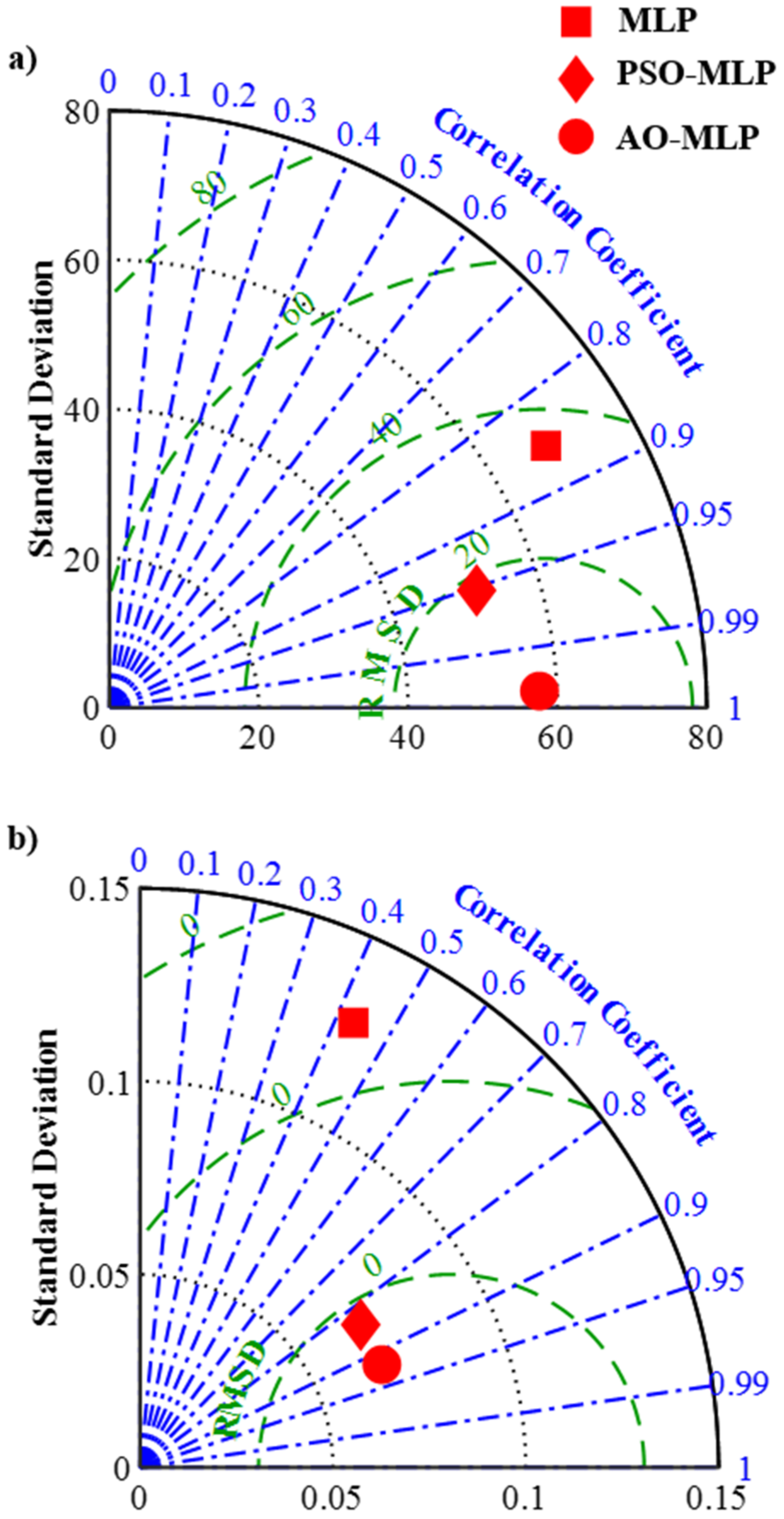
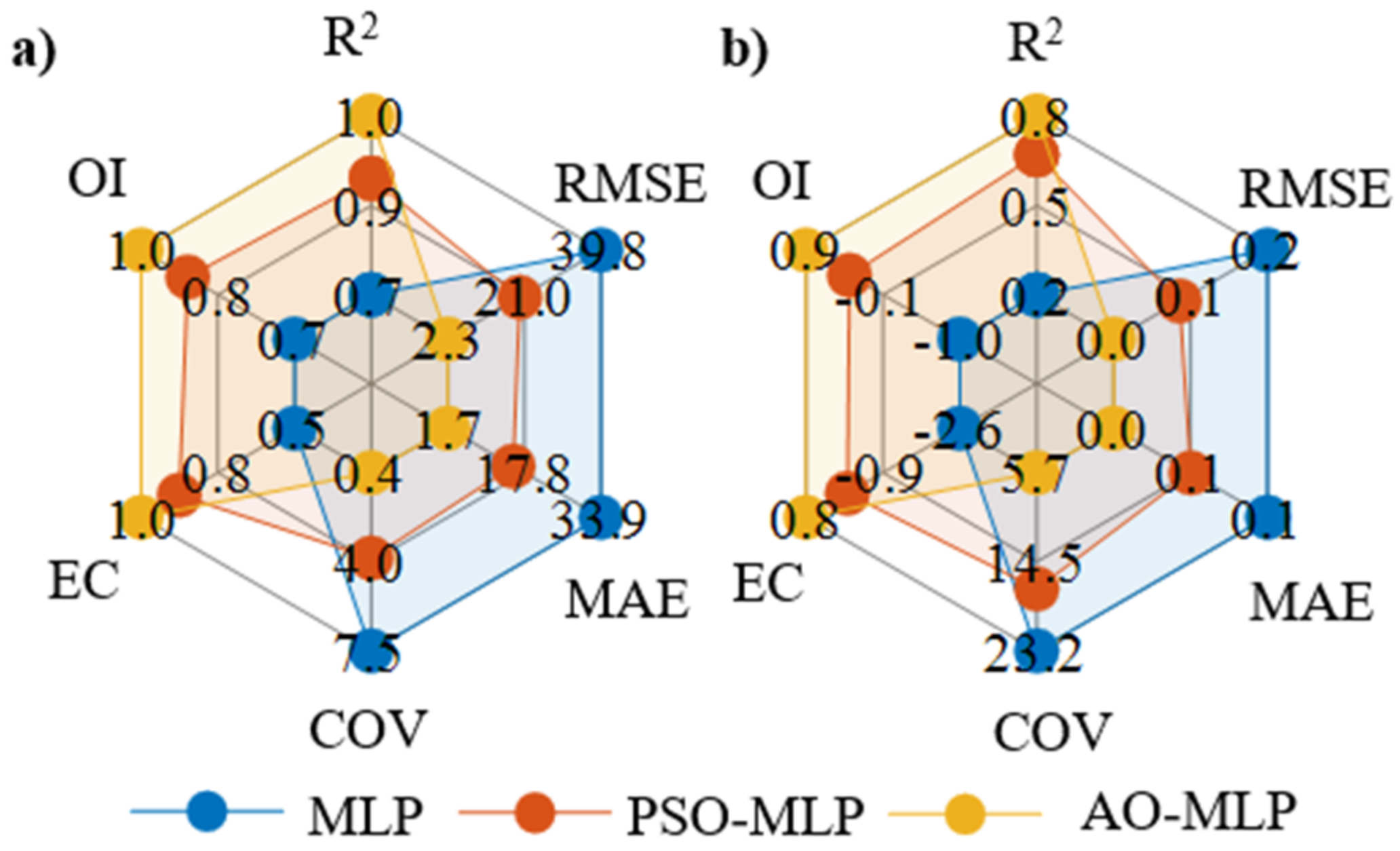
| R2 | RMSE | MAE | COV | EC | OI | ||
| Shear strength | MLP | 0.735 | 39.798 | 33.925 | 7.523 | 0.531 | 0.684 |
| PSO-MLP | 0.907 | 19.909 | 15.462 | 3.839 | 0.882 | 0.901 | |
| AO-MLP | 0.998 | 2.283 | 1.729 | 0.447 | 0.998 | 0.994 | |
| Seam Width | MLP | 0.187 | 0.153 | 0.127 | 23.198 | −2.602 | −1.002 |
| PSO-MLP | 0.705 | 0.084 | 0.075 | 17.117 | −0.084 | 0.347 | |
| AO-MLP | 0.847 | 0.0321 | 0.023 | 5.708 | 0.841 | 0.878 | |
Disclaimer/Publisher’s Note: The statements, opinions and data contained in all publications are solely those of the individual author(s) and contributor(s) and not of MDPI and/or the editor(s). MDPI and/or the editor(s) disclaim responsibility for any injury to people or property resulting from any ideas, methods, instructions or products referred to in the content. |
© 2023 by the authors. Licensee MDPI, Basel, Switzerland. This article is an open access article distributed under the terms and conditions of the Creative Commons Attribution (CC BY) license (https://creativecommons.org/licenses/by/4.0/).
Share and Cite
Moustafa, E.B.; Elsheikh, A. Predicting Characteristics of Dissimilar Laser Welded Polymeric Joints Using a Multi-Layer Perceptrons Model Coupled with Archimedes Optimizer. Polymers 2023, 15, 233. https://doi.org/10.3390/polym15010233
Moustafa EB, Elsheikh A. Predicting Characteristics of Dissimilar Laser Welded Polymeric Joints Using a Multi-Layer Perceptrons Model Coupled with Archimedes Optimizer. Polymers. 2023; 15(1):233. https://doi.org/10.3390/polym15010233
Chicago/Turabian StyleMoustafa, Essam B., and Ammar Elsheikh. 2023. "Predicting Characteristics of Dissimilar Laser Welded Polymeric Joints Using a Multi-Layer Perceptrons Model Coupled with Archimedes Optimizer" Polymers 15, no. 1: 233. https://doi.org/10.3390/polym15010233