
Experimental Investigation of Shale Tensile Failure under Thermally Conditioned Linear Fracturing Fluid (LFF) System and Reservoir Temperature Controlled Conditions


Abstract
:
1. Introduction
2. Statement of Theories
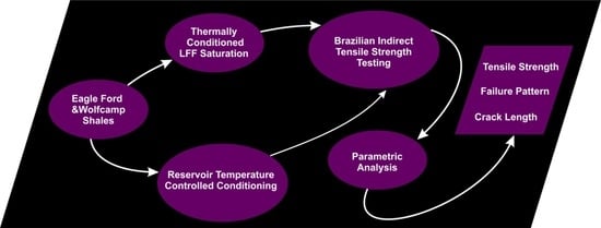
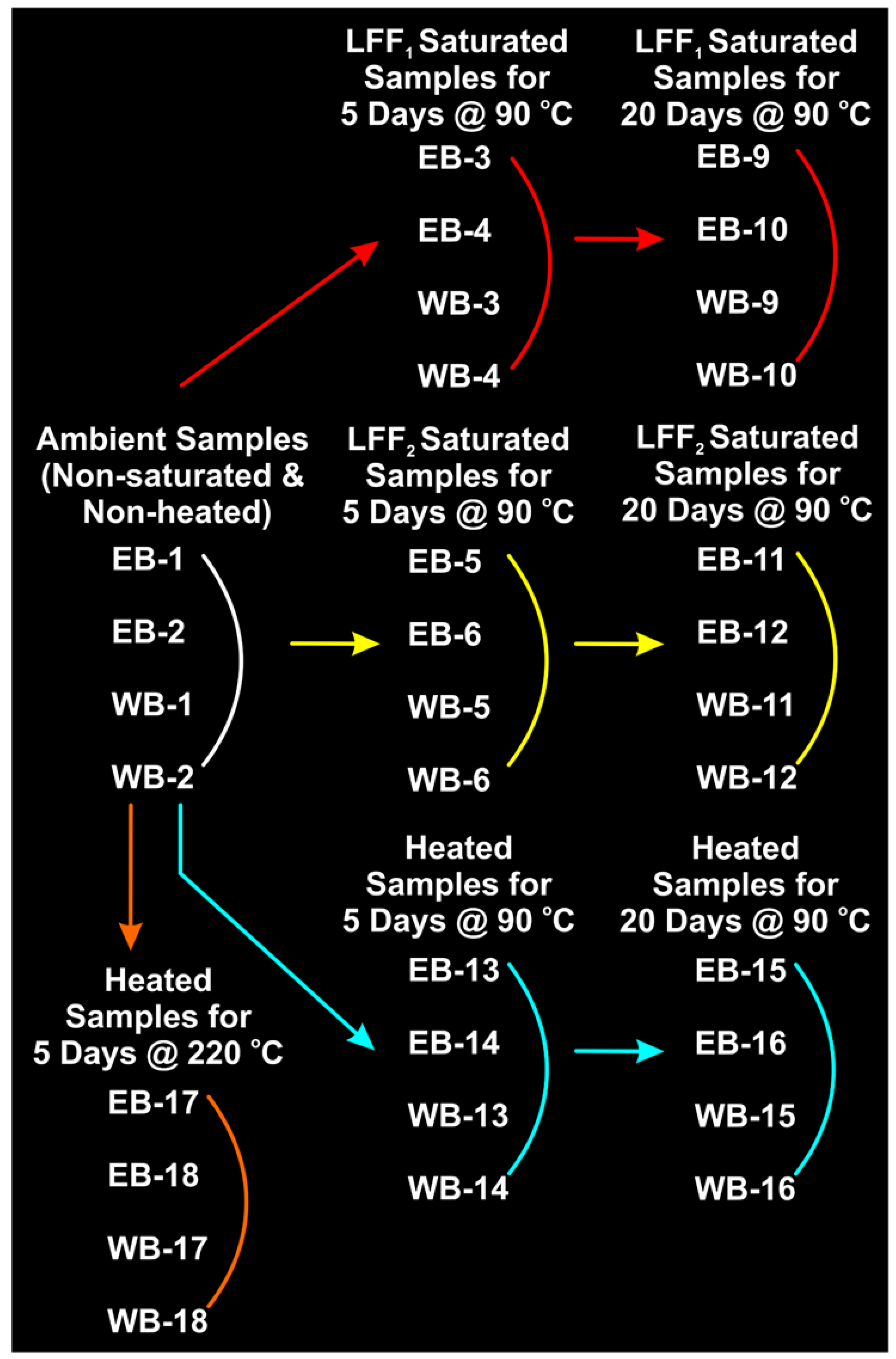
3. Methodology
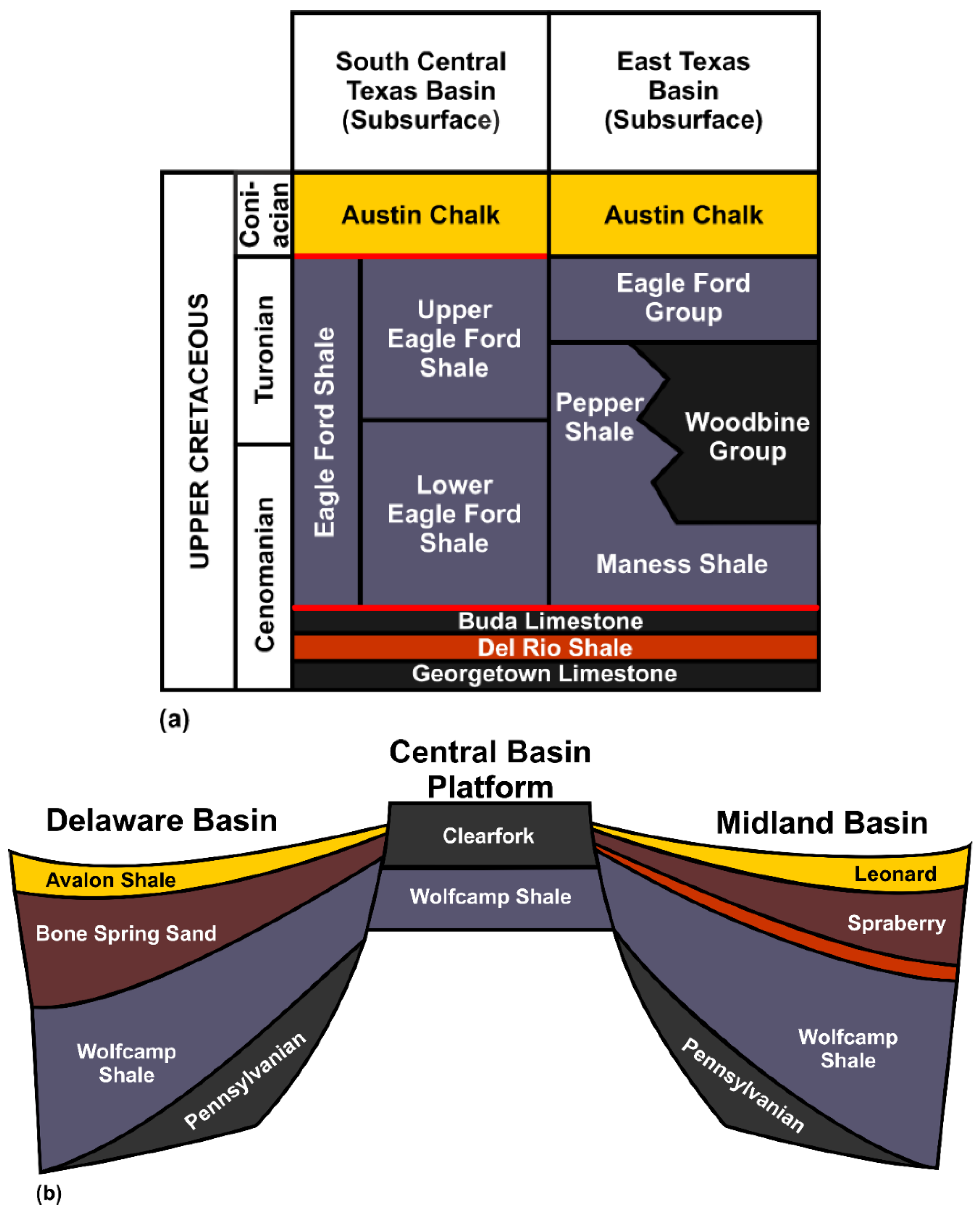
3.1. Geological Setting
3.2. Samples Characterization
3.3. Fluid Preparation and Shale Samples’ Treatment
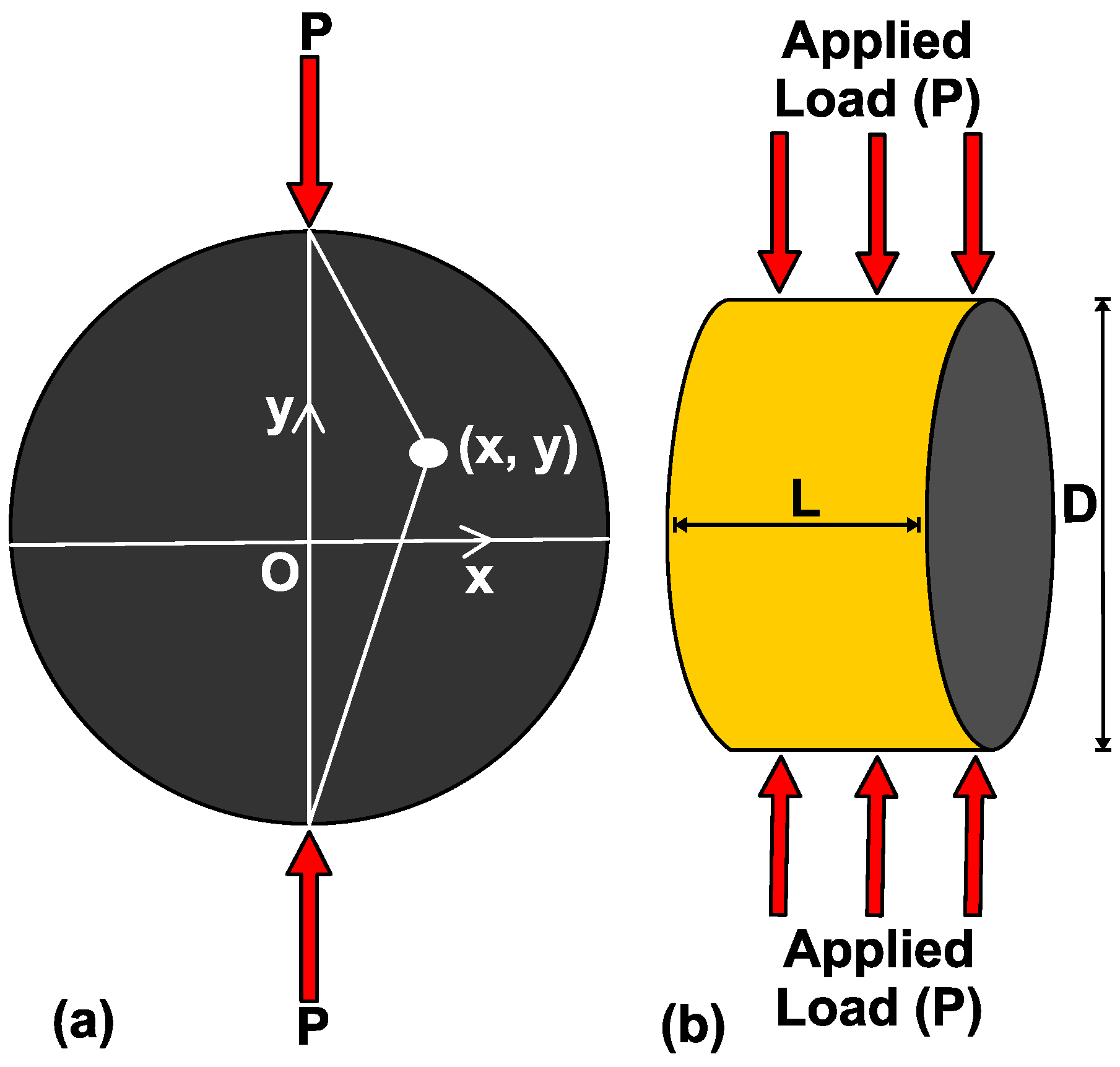
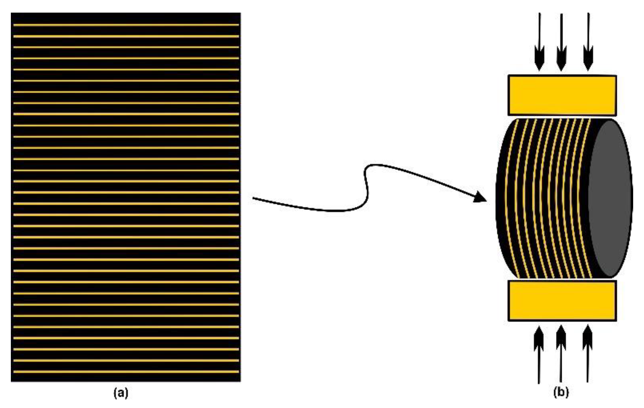
3.4. Brazilian Indirect Tensile Strength Testing
4. Results Analysis and Discussion
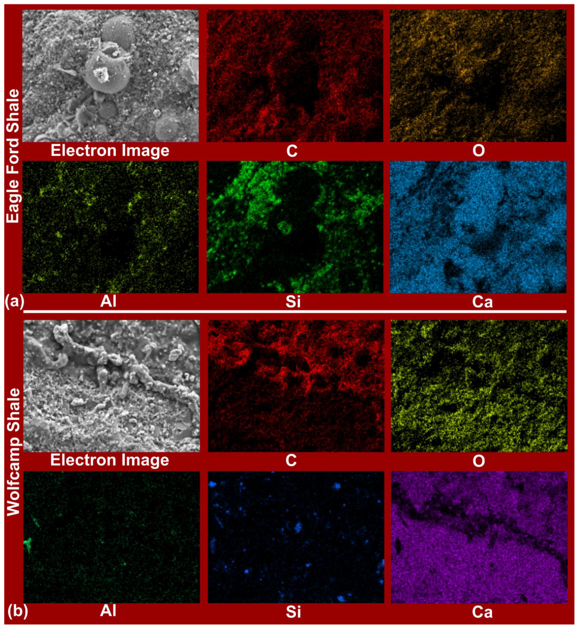
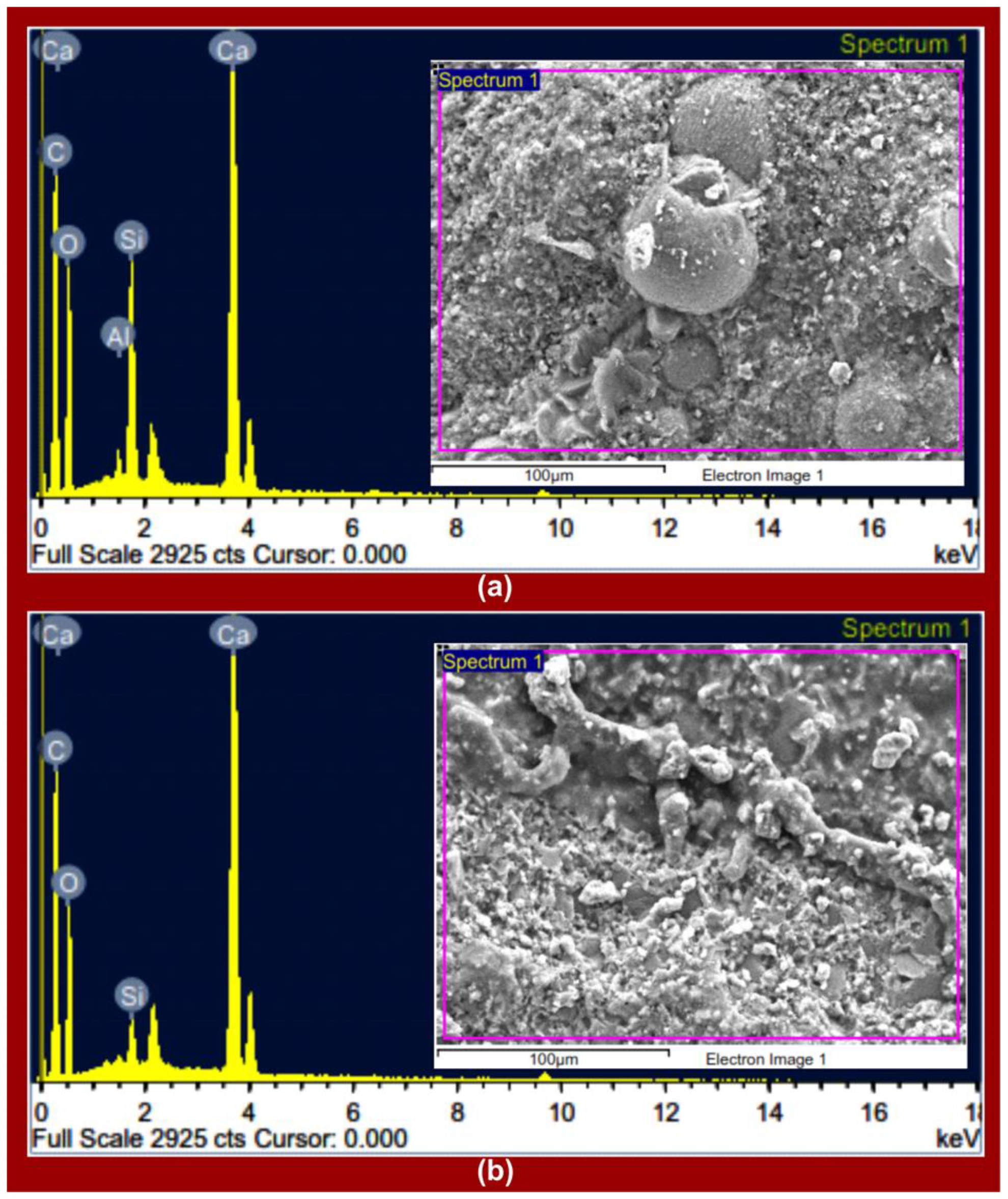
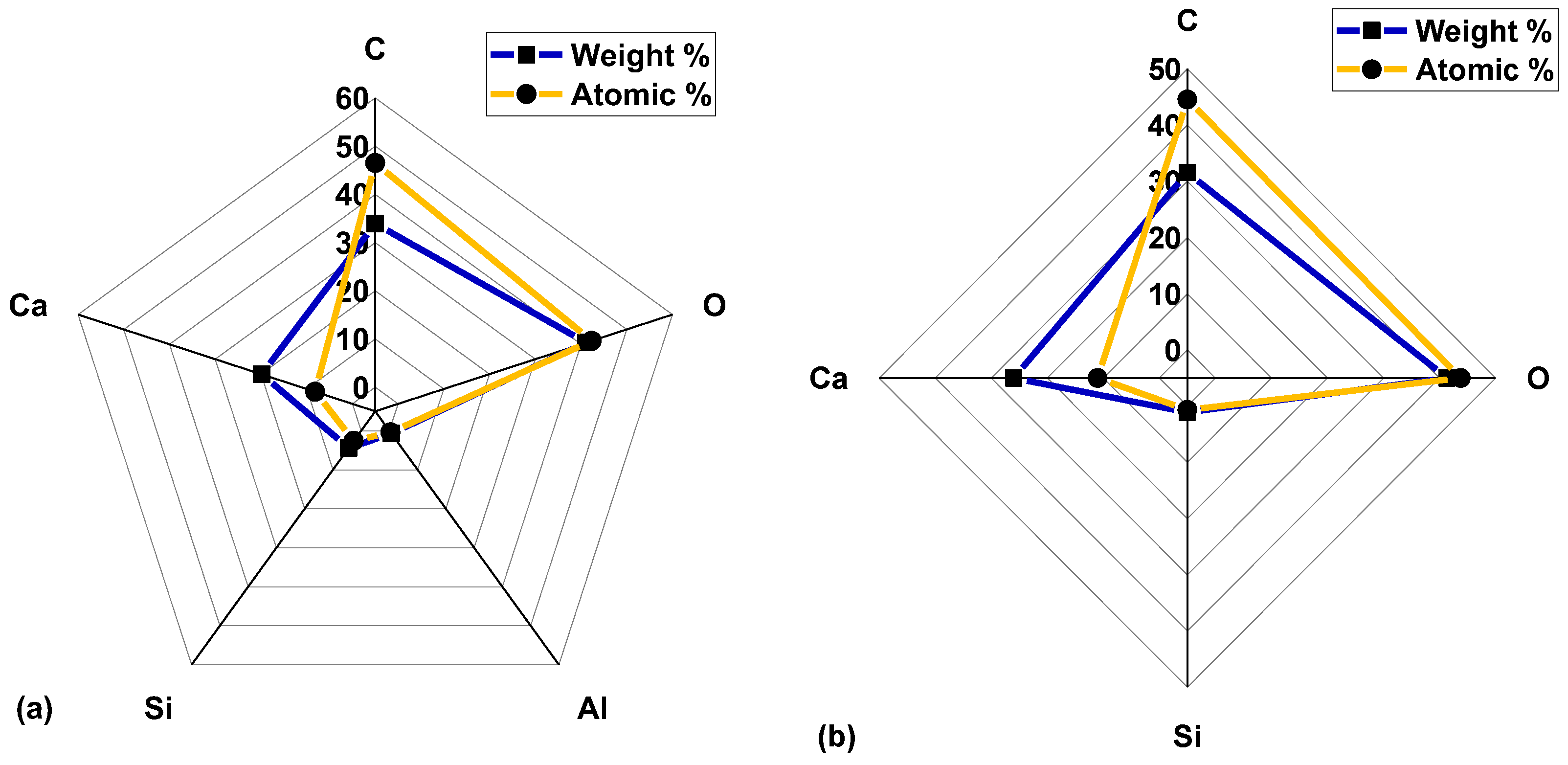
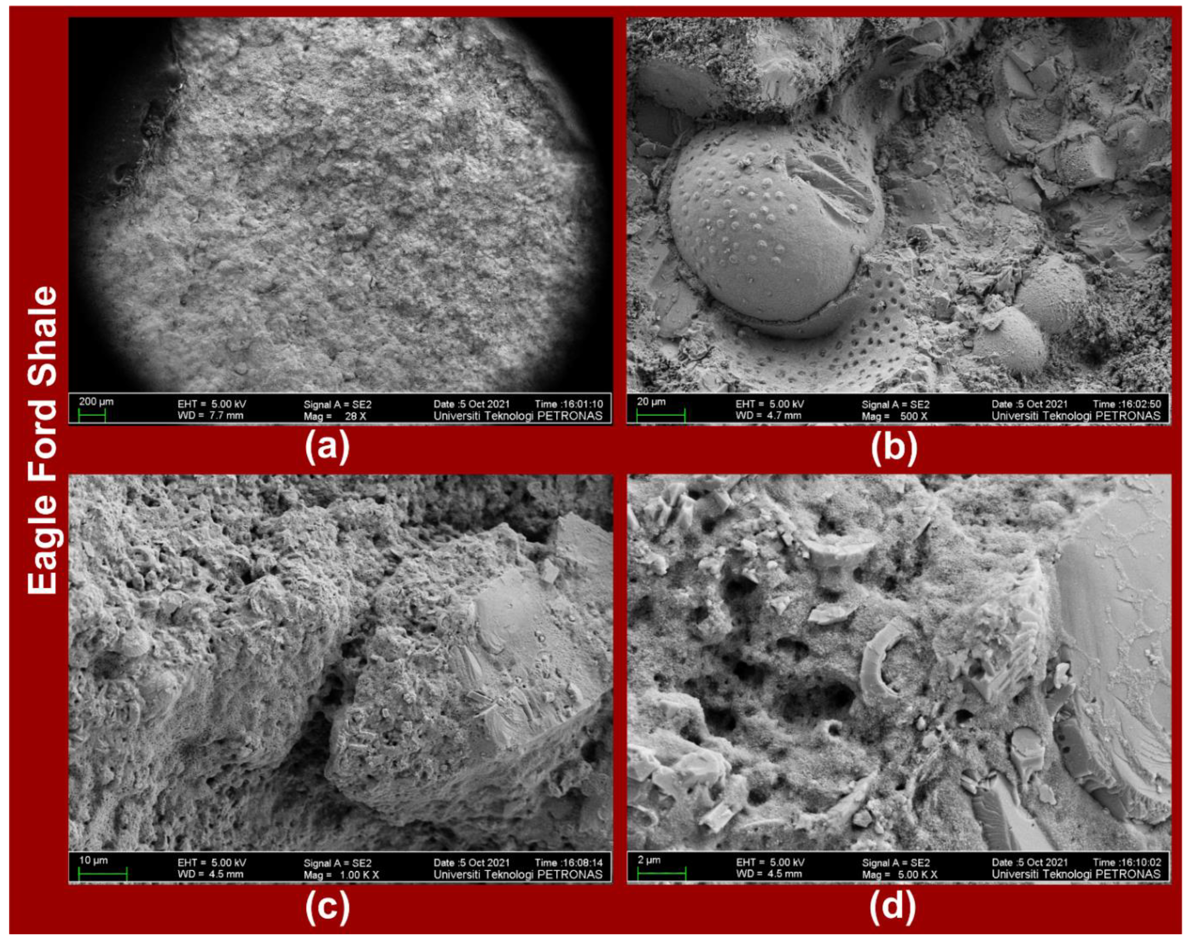
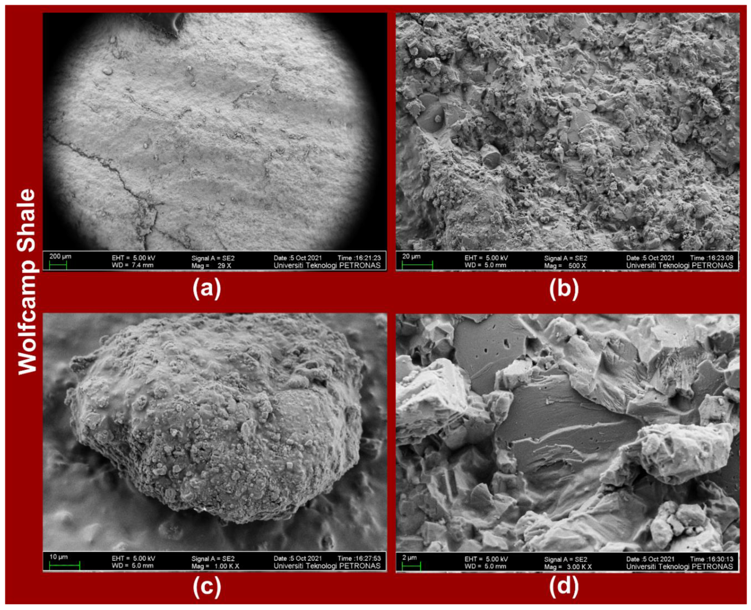
4.1. FESEM-EDX-Mapping Analysis of Eagle Ford and Wolfcamp Shales
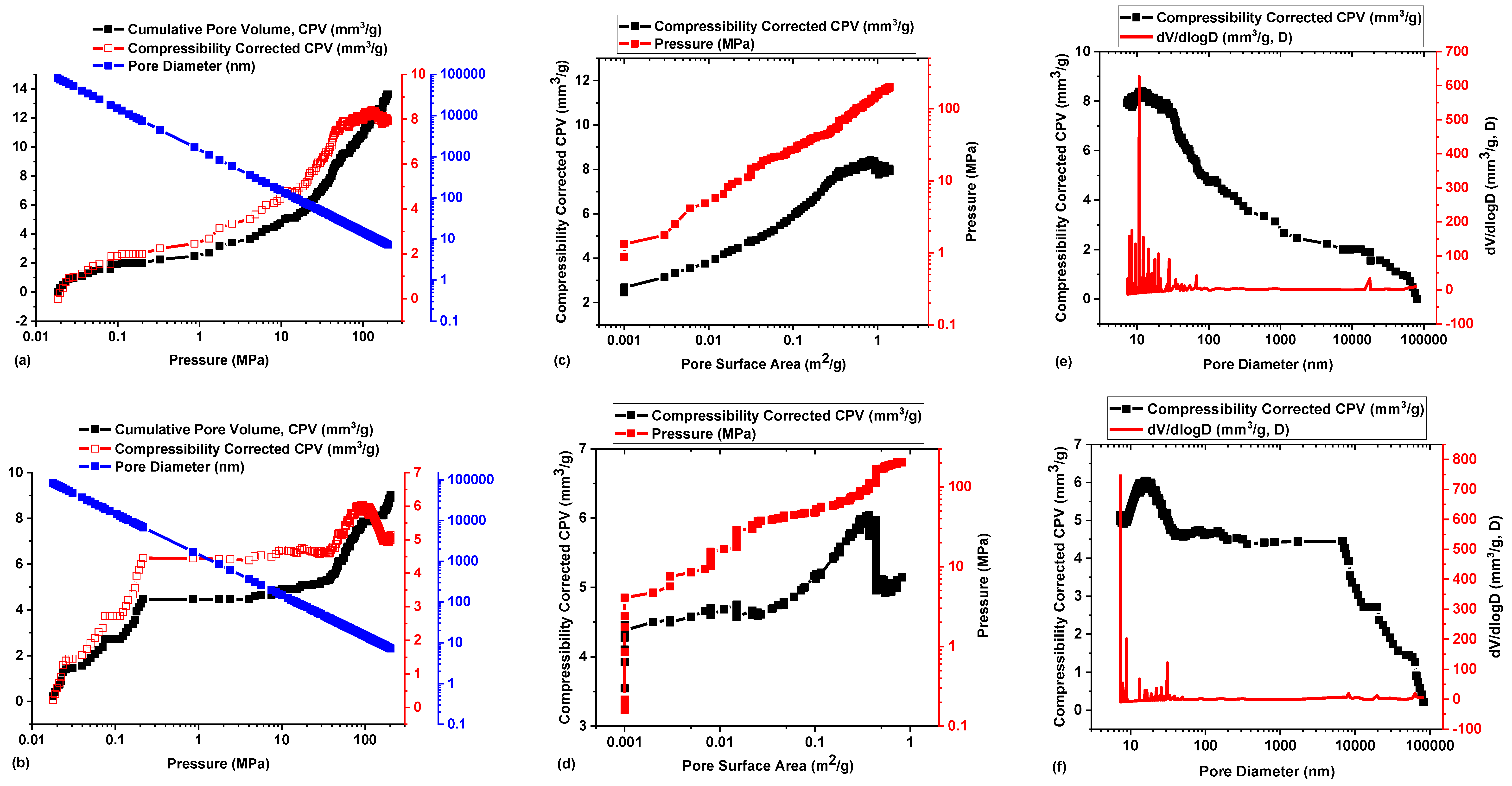
4.2. Porosity—Permeability Characterization of Eagle Ford and Wolfcamp Shales
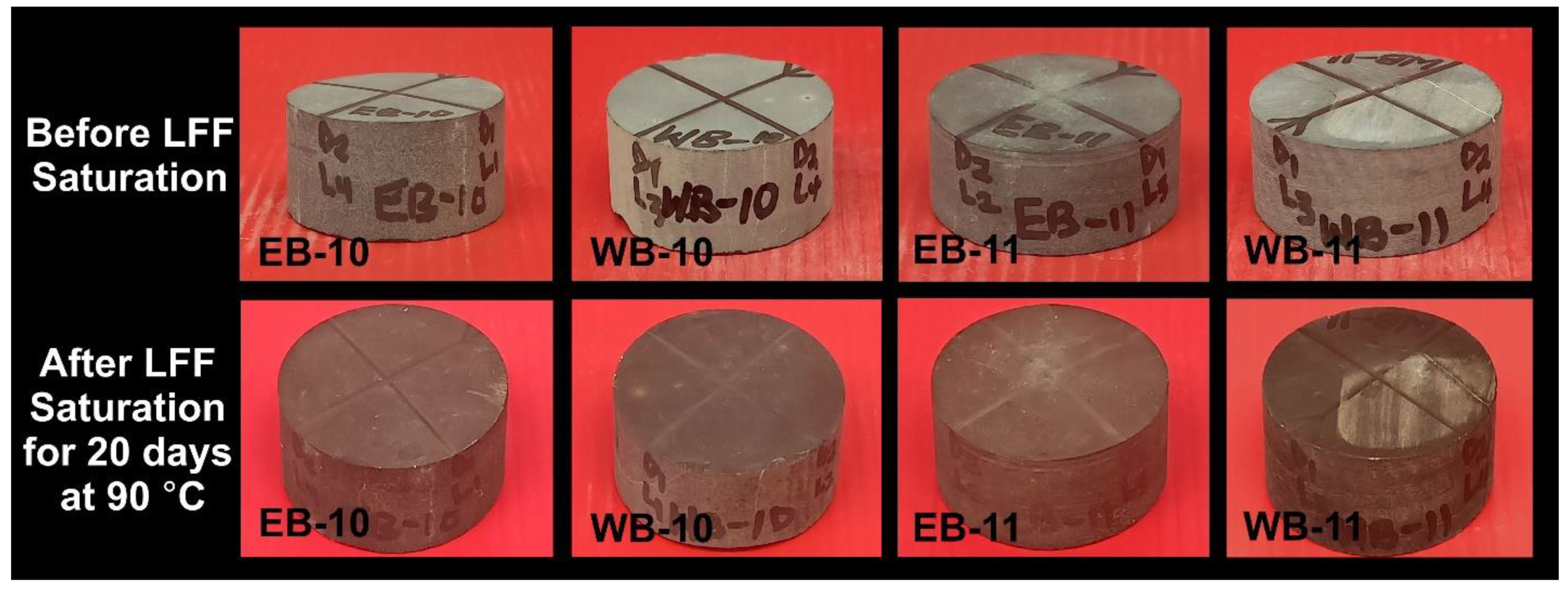
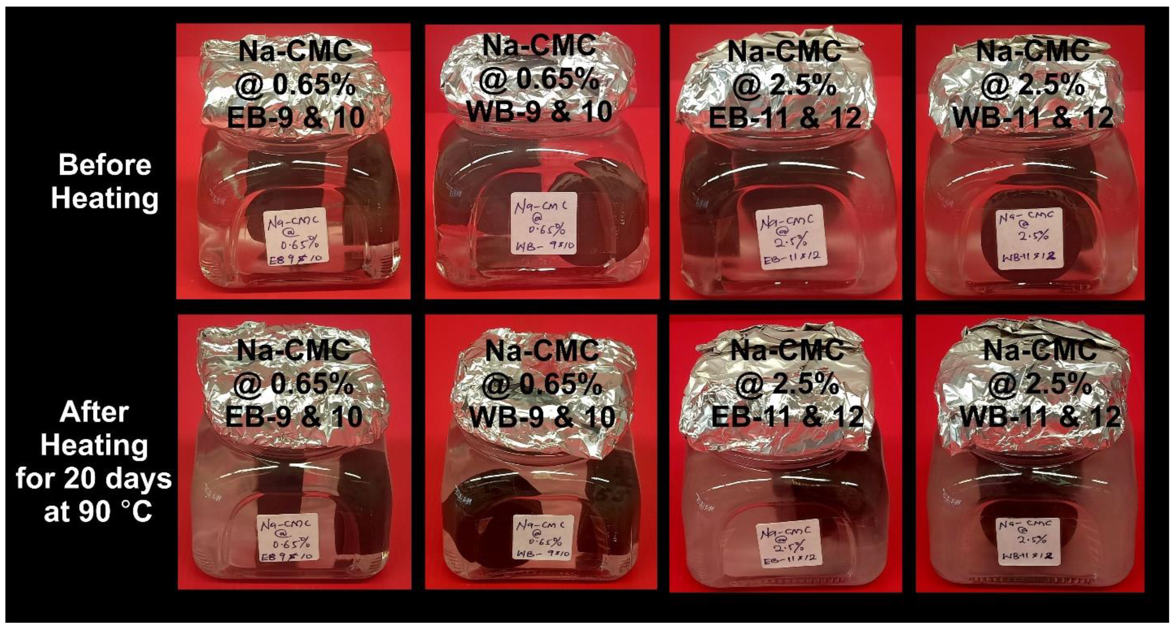
4.3. Thermal Conditioning Effects on Physical Appearances of Shale and LFF
4.4. Tensile Strength and Failure Analysis of Eagle Ford and Wolfcamp Shales
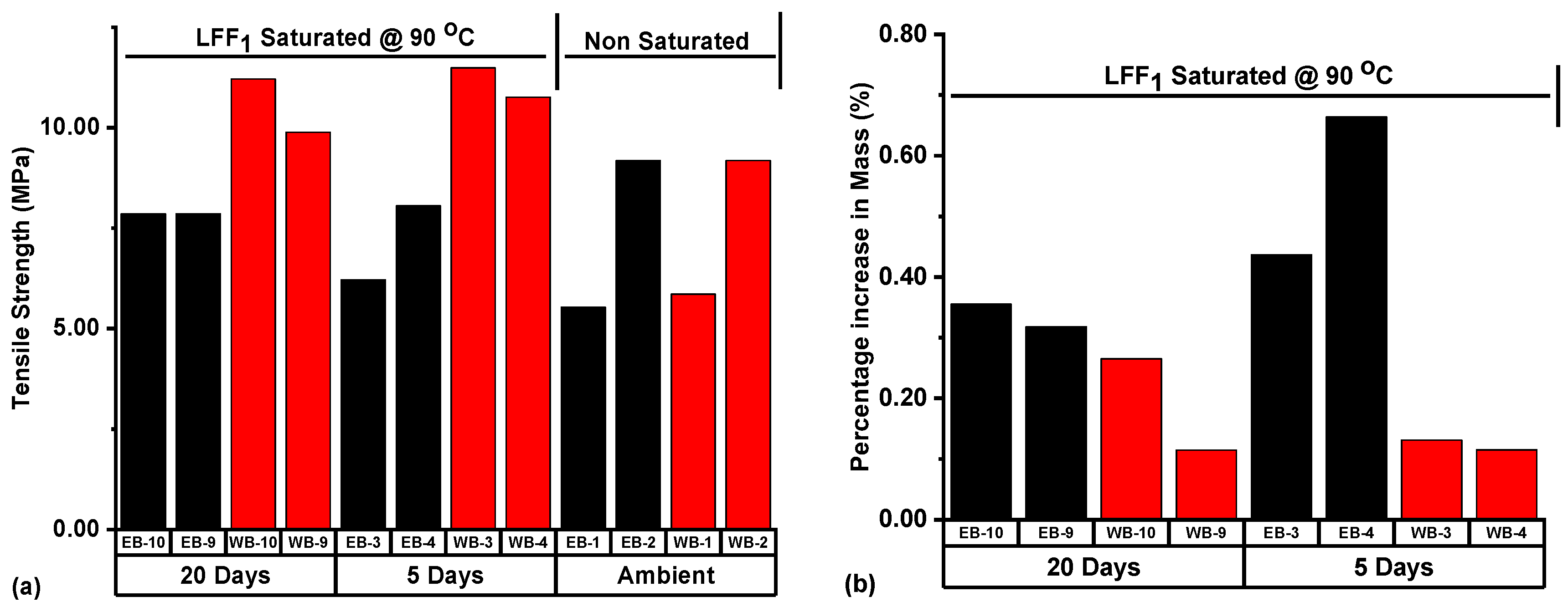
4.4.1. Tensile Strength and Failure Analysis of Thermally Conditioned LFF1 Saturated Samples
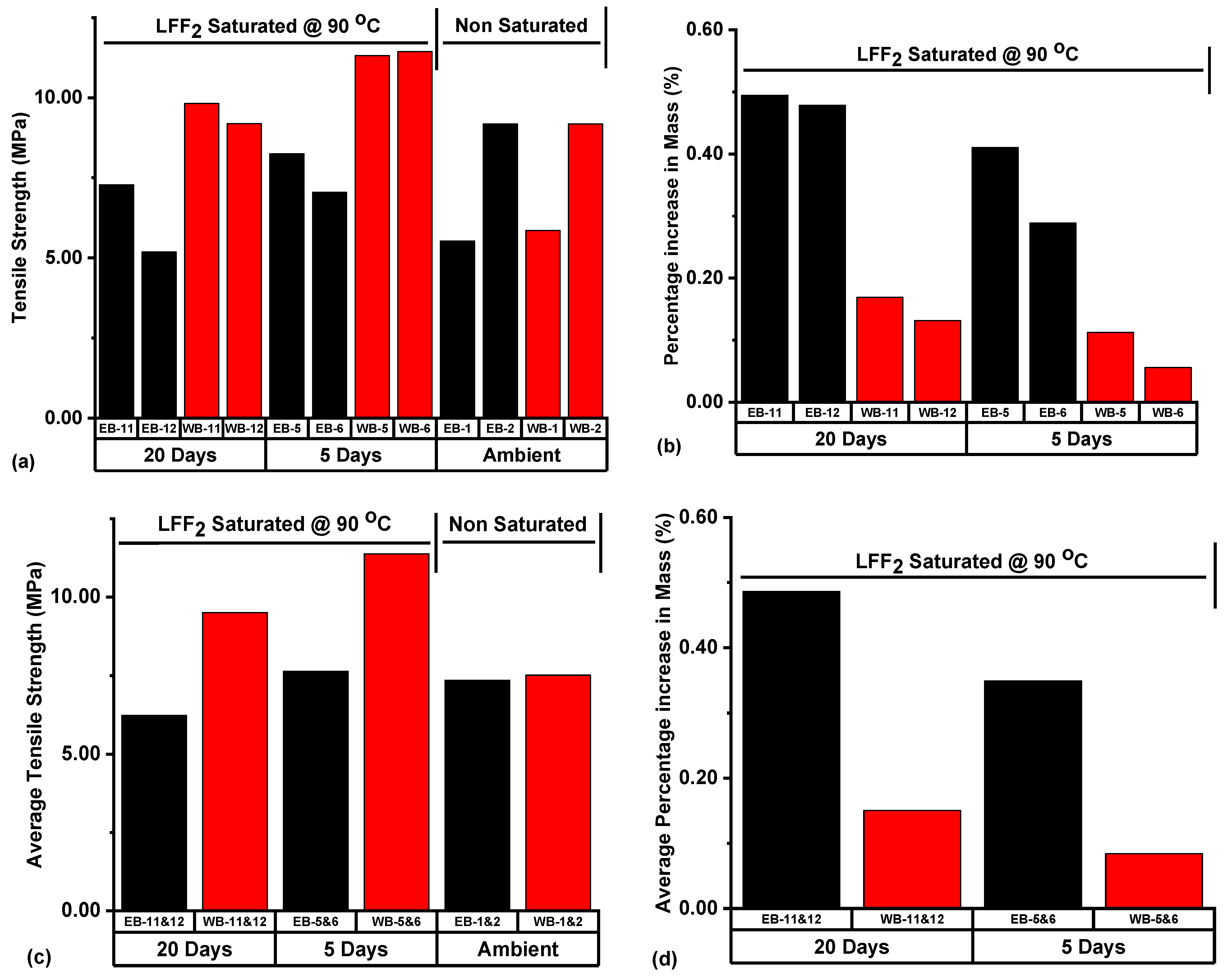
4.4.2. Tensile Strength and Failure Analysis of LFF2 Saturated Samples
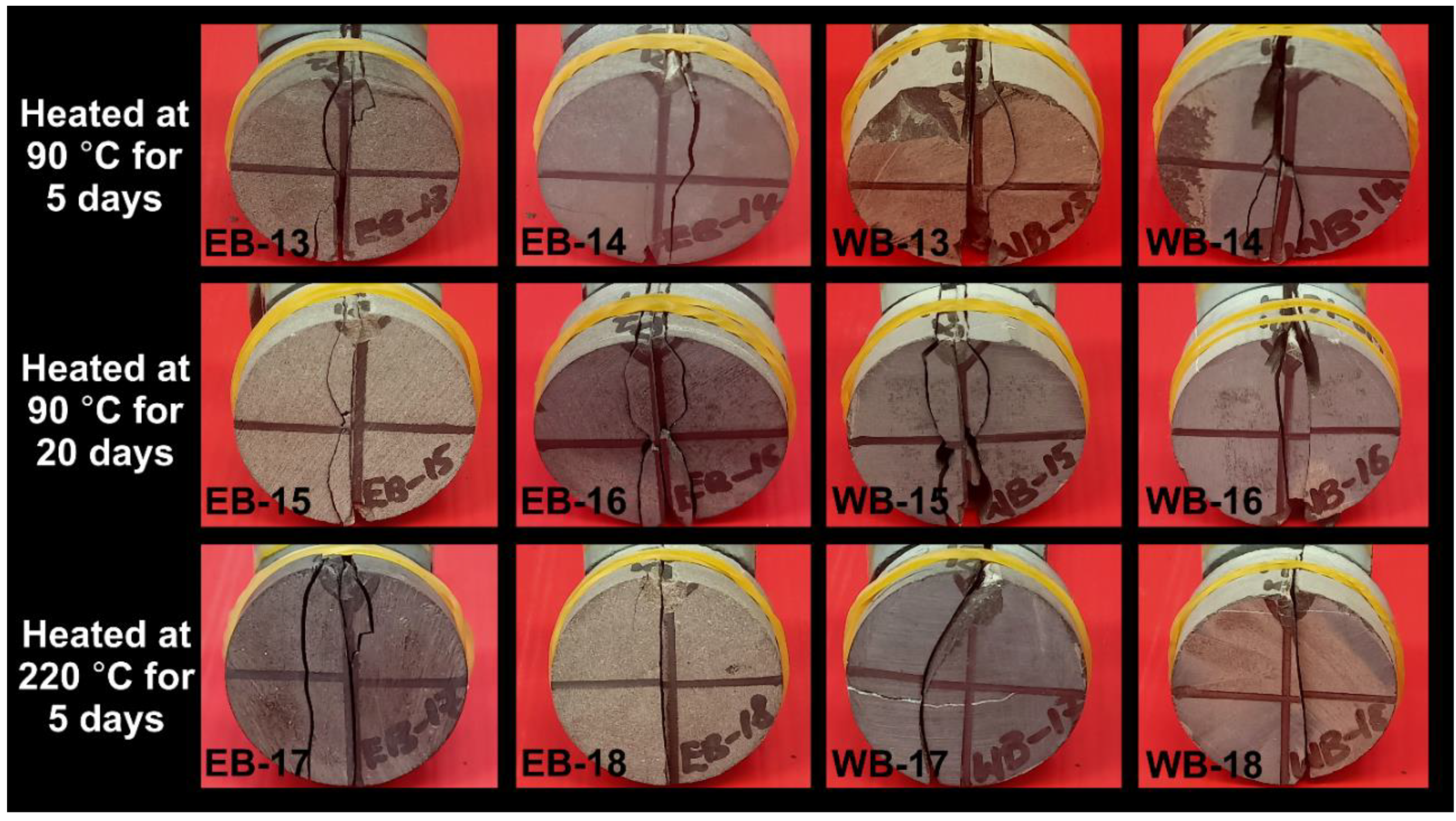
4.4.3. Tensile Strength and Failure Analysis of Reservoir Temperature Conditioned Samples
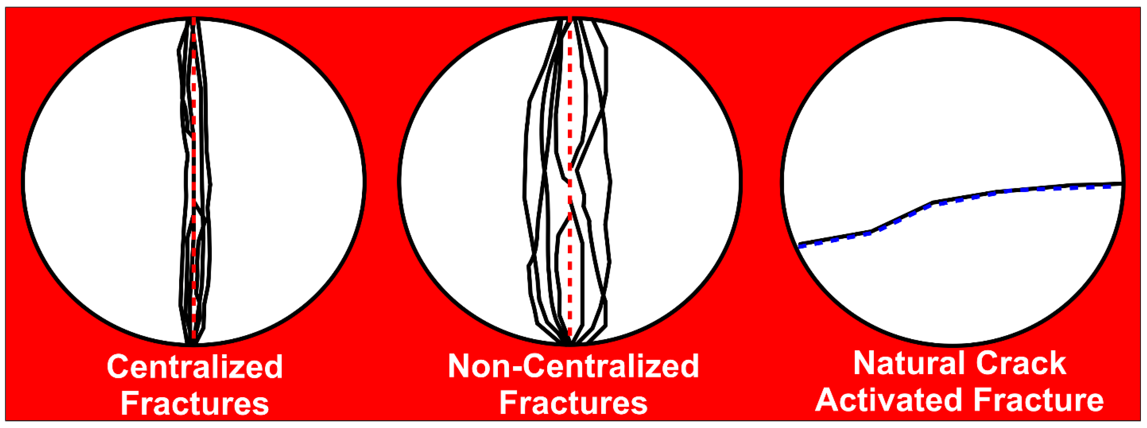
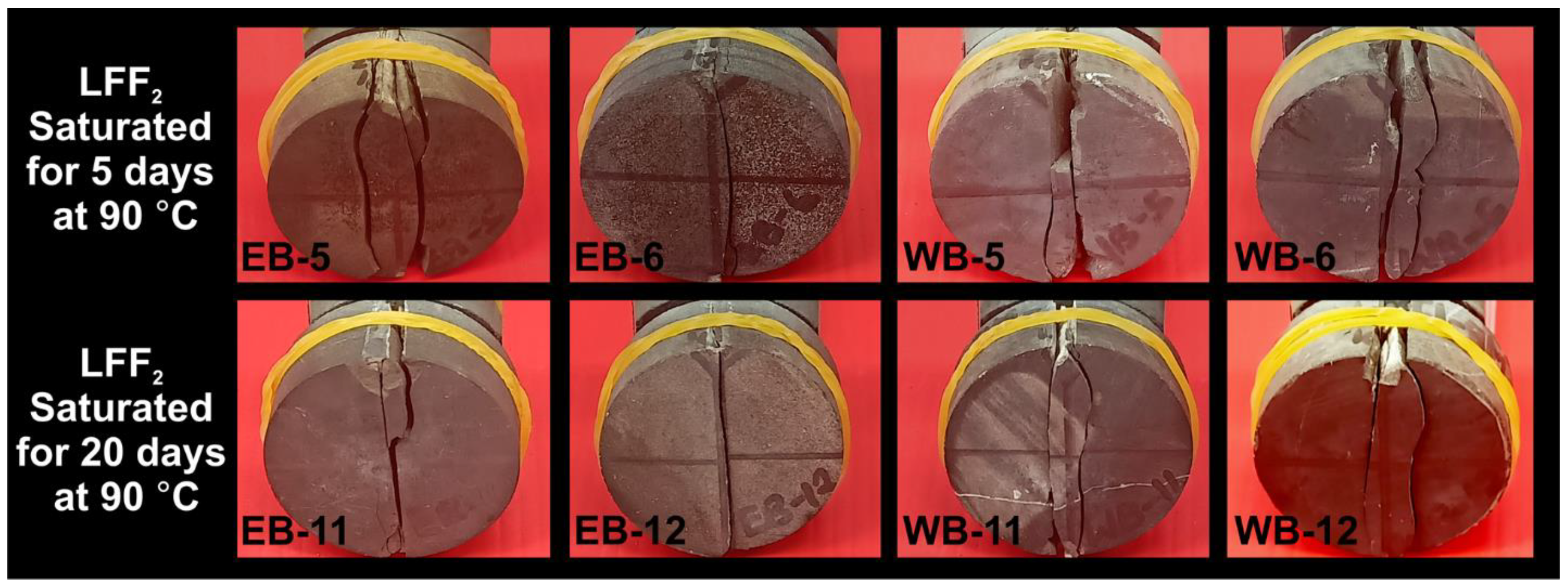
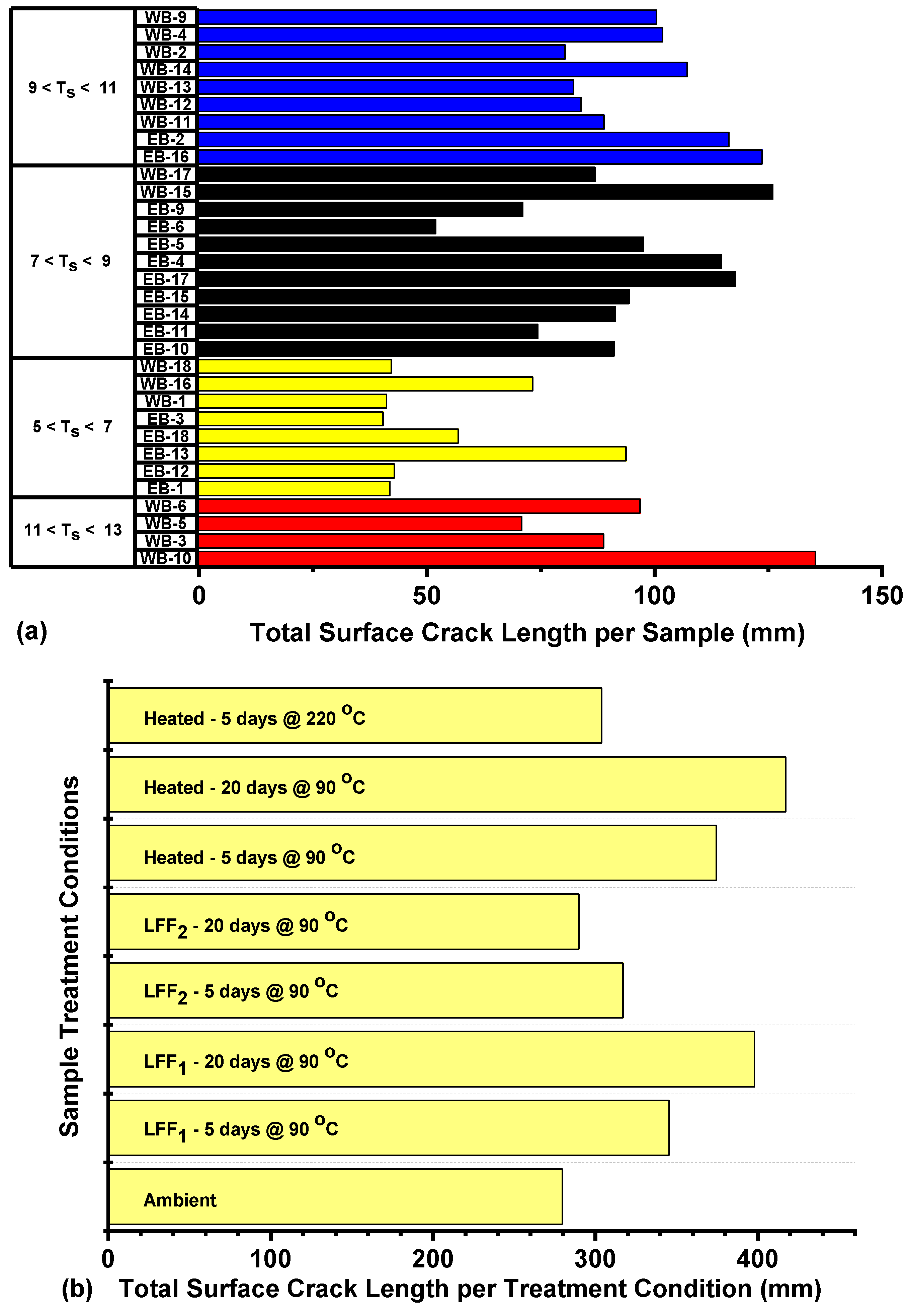
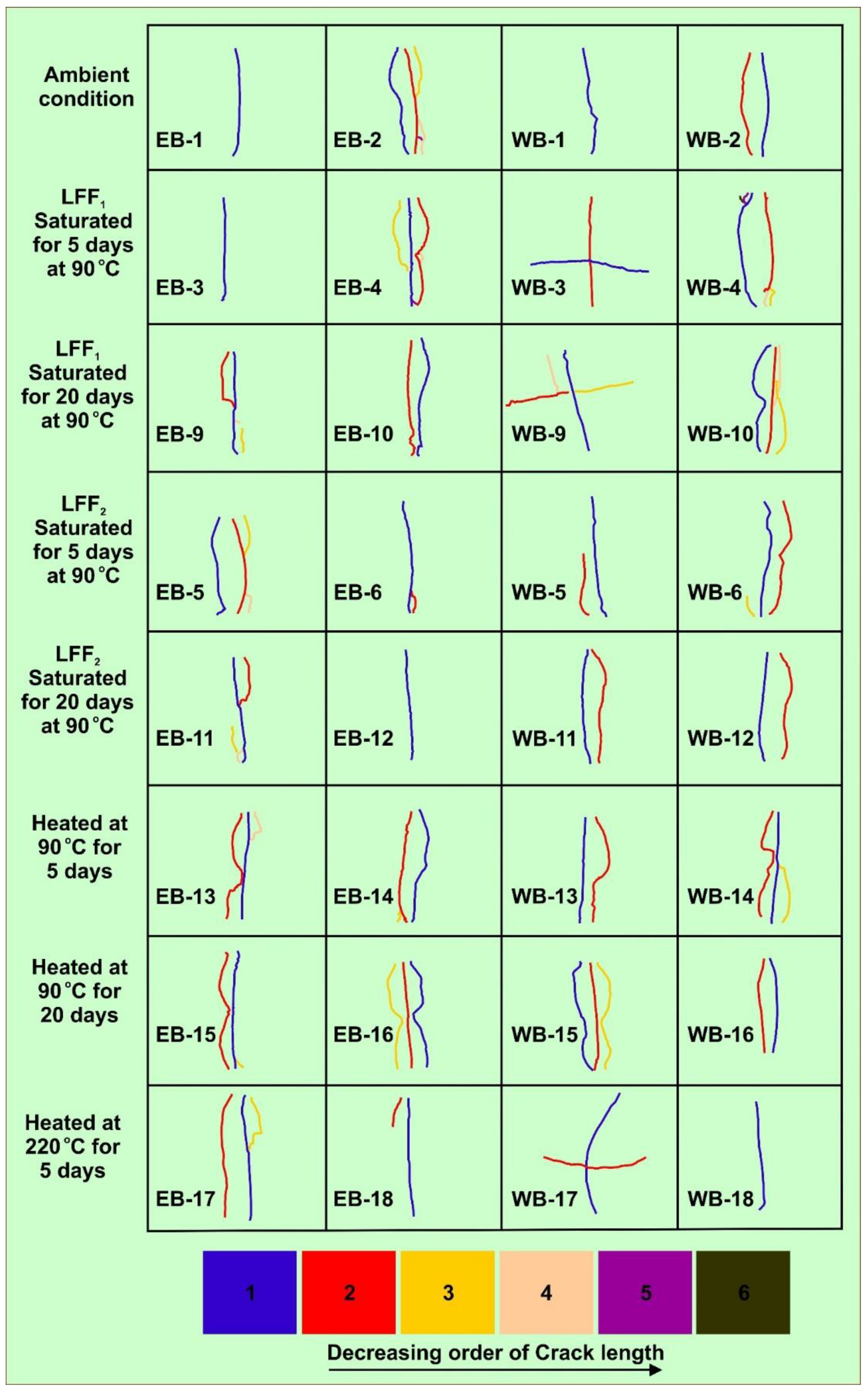
4.4.4. Failure Crack Length Analysis
4.5. Discussion of Results
5. Conclusions
Supplementary Materials
Author Contributions
Funding
Institutional Review Board Statement
Informed Consent Statement
Data Availability Statement
Acknowledgments
Conflicts of Interest
References
- Acosta, J.C.; Dang, S.; Curtis, M.; Sondergeld, C.; Rai, C. Fracturing Fluids Effect on Mechanical Properties in Shales. In Proceedings of the 8th Unconventional Resources Technology Conference, Austin, TX, USA, 20–22 July 2020. [Google Scholar] [CrossRef]
- Gandossi, L. An Overview of Hydraulic Fracturing and Other Formation Stimulation Technologies for Shale Gas Production; JRC98582; European Union: Luxembourg, 2013. [Google Scholar] [CrossRef]
- Gu, M.; Mohanty, K.K. Rheology of polymer-free foam fracturing fluids. J. Pet. Sci. Eng. 2015, 134, 87–96. [Google Scholar] [CrossRef]
- Barati, R.; Liang, J.-T. A review of fracturing fluid systems used for hydraulic fracturing of oil and gas wells. J. Appl. Polym. Sci. 2014, 131, 40735. [Google Scholar] [CrossRef]
- Chauhan, G.; Verma, A.; Doley, A.; Ojha, K. Rheological and breaking characteristics of Zr-crosslinked gum karaya gels for high-temperature hydraulic fracturing application. J. Pet. Sci. Eng. 2018, 172, 327–339. [Google Scholar] [CrossRef]
- Aliu, A.O.; Guo, J.; Wang, S.; Zhao, X. Hydraulic fracture fluid for gas reservoirs in petroleum engineering applications using sodium carboxy methyl cellulose as gelling agent. J. Nat. Gas Sci. Eng. 2016, 32, 491–500. [Google Scholar] [CrossRef]
- Al-Hajri, S.; Negash, B.M.; Rahman, M.; Haroun, M.; Al-Shami, T.M. Perspective Review of Polymers as Additives in Water-Based Fracturing Fluids. ACS Omega 2022, 7, 7431–7443. [Google Scholar] [CrossRef]
- Al-Muntasheri, G. A Critical Review of Hydraulic Fracturing Fluids over the Last Decade. In Proceedings of the SPE Western North America and Rocky Mountain Joint Regional Meeting, Denver, CO, USA, 16–18 April 2014; pp. 16–18. [Google Scholar]
- Lufeng, Z.; Fujian, Z.; Shicheng, Z.; Zhun, L.; Jin, W.; Yuechun, W. Evaluation of permeability damage caused by drilling and fracturing fluids in tight low permeability sandstone reservoirs. J. Pet. Sci. Eng. 2019, 175, 1122–1135. [Google Scholar] [CrossRef]
- Akrad, O.M.; Miskimins, J.L.; Prasad, M. The Effects of Fracturing Fluids on Shale Rock Mechanical Properties and Proppant Embedment. In Proceedings of the SPE Annual Technical Conference and Exhibition, Denver, CO, USA, 30 October–2 November 2011; pp. 2245–2256. [Google Scholar] [CrossRef] [Green Version]
- Duan, K.; Kwok, C. Discrete element modeling of anisotropic rock under Brazilian test conditions. Int. J. Rock Mech. Min. Sci. 2015, 78, 46–56. [Google Scholar] [CrossRef]
- Li, H.; Lai, B.; Liu, H.-H.; Zhang, J.; Georgi, D. Experimental Investigation on Brazilian Tensile Strength of Organic-Rich Gas Shale. SPE J. 2017, 22, 148–161. [Google Scholar] [CrossRef]
- Ma, T.; Peng, N.; Zhu, Z.; Zhang, Q.; Yang, C.; Zhao, J. Brazilian Tensile Strength of Anisotropic Rocks: Review and New Insights. Energies 2018, 11, 304. [Google Scholar] [CrossRef] [Green Version]
- Jaeger, J.C.; Cook, N.G.W.; Zimmerman, R.W. Fundamentals of Rock Mechanics, 4th ed.; Blackwell Publishing: Oxford, UK, 2007. [Google Scholar] [CrossRef]
- ASTM D3967-16; Splitting Tensile Strength of Intact Rock Core Specimens 1. ASTM International: West Conshohocken, PA, USA, 2001.
- Chen, C.S.; Hsu, S.C. Measurement of Indirect Tensile Strength of Anisotropic Rocks by the Ring Test. Rock Mech. Rock Eng. 2001, 34, 293–321. [Google Scholar] [CrossRef]
- Lai, B.T.; Li, H.; Liu, H.H.; Zhang, J.L.; Georgi, D. Brazilian Tensile Strength Test of Orgainc-Rich Shale. In Proceedings of the SPE Abu Dhabi International Petroleum Exhibition and Conference, Abu Dhabi, UAE, 15–18 November 2015; pp. 1–20. [Google Scholar] [CrossRef]
- Lin, W. Mechanical Properties of Mesaverde Shale and Sandstone at High Pressure. In Proceedings of the AIRAPT Conference on High Pressure and 19 EHPRG Conference, Uppsala, Sweden, 17–22 August 1981; pp. 736–739. [Google Scholar]
- Chong, K.P.; Chen, J.L.; Dana, G.F.; Weber, J.A. Indirect and Direct Tensile Behaviour of Devonian Oil Shales; Dept. of Civil Engineering, University of Wyoming: Laramie, WY, USA, 1984. [Google Scholar]
- Mokhtari, M.; Honarpour, M.M.; Tutuncu, A.N.; Boitnott, G.N. Acoustical and Geomechanical Characterization of Eagle Ford Shale—Anisotropy, Heterogeneity and Measurement Scale. In Proceedings of the SPE Annual Technical Conference and Exhibition, Amsterdam, The Netherlands, 27–29 October 2014; pp. 1–19. [Google Scholar] [CrossRef]
- Gao, Q.; Tao, J.; Hu, J.; Yu, X. Laboratory study on the mechanical behaviors of an anisotropic shale rock. J. Rock Mech. Geotech. Eng. 2015, 7, 213–219. [Google Scholar] [CrossRef] [Green Version]
- He, J.; Afolagboye, L.O. Influence of layer orientation and interlayer bonding force on the mechanical behavior of shale under Brazilian test conditions. Acta Mech. Sin. Xuebao 2017, 34, 349–358. [Google Scholar] [CrossRef]
- Hou, B.; Zeng, Y.; Fan, M.; Li, D. Brittleness Evaluation of Shale Based on the Brazilian Splitting Test. Geofluids 2018, 2018, 3602852. [Google Scholar] [CrossRef] [Green Version]
- Simpson, N.D.J.; Stroisz, A.; Bauer, A.; Vervoort, A.; Holt, R.M. Failure mechanics of anisotropic shale during Brazilian tests. In 48th US Rock Mechanics/Geomechanics Symposium Proceedings; American Rock Mechanics Association (ARMA): Minneapolis, MN, USA, 2014; Volume 1, pp. 228–240. [Google Scholar]
- Wang, J.; Xie, L.; Xie, H.; Ren, L.; He, B.; Li, C.; Yang, Z.; Gao, C. Effect of layer orientation on acoustic emission characteristics of anisotropic shale in Brazilian tests. J. Nat. Gas Sci. Eng. 2016, 36, 1120–1129. [Google Scholar] [CrossRef]
- Yang, S.-Q.; Yin, P.-F.; Huang, Y.-H. Experiment and Discrete Element Modelling on Strength, Deformation and Failure Behaviour of Shale Under Brazilian Compression. Rock Mech. Rock Eng. 2019, 52, 4339–4359. [Google Scholar] [CrossRef]
- Vernik, L.; Nur, A. Ultrasonic velocity and anisotropy of hydrocarbon source rocks. Geophysics 1992, 57, 727–735. [Google Scholar] [CrossRef]
- Amadei, B.; Jonsson, T. Tensile strength of anisotropic rocks measured with the splitting tension test. In Proceedings of the 12th Southeastern Conference Theoretical and Applied Mechanics, Pine Mountain, GA, USA, 10–11 May 1984; p. 1984. [Google Scholar]
- Chen, C.-S.; Pan, E.; Amadei, B. Determination of deformability and tensile strength of anisotropic rock using Brazilian tests. Int. J. Rock Mech. Min. Sci. 1998, 35, 43–61. [Google Scholar] [CrossRef]
- Lekhnitskii, S.G.; Tsai, S.W.; Cheron, T. Anisotropic Plates, 1st ed.; Gordon and Breach Science Publishers: New York, NY, USA, 1968. [Google Scholar]
- Claesson, J.; Bohloli, B. Brazilian test: Stress field and tensile strength of anisotropic rocks using an analytical solution. Int. J. Rock Mech. Min. Sci. 2002, 39, 991–1004. [Google Scholar] [CrossRef]
- Lee, Y.-K.; Pietruszczak, S. Tensile failure criterion for transversely isotropic rocks. Int. J. Rock Mech. Min. Sci. 2015, 79, 205–215. [Google Scholar] [CrossRef]
- Cho, J.-W.; Kim, H.; Jeon, S.; Min, K.-B. Deformation and strength anisotropy of Asan gneiss, Boryeong shale, and Yeoncheon schist. Int. J. Rock Mech. Min. Sci. 2012, 50, 158–169. [Google Scholar] [CrossRef]
- Mighani, S.; Sondergeld, C.H.; Rai, C.S. Observations of Tensile Fracturing of Anisotropic Rocks. SPE J. 2016, 21, 1289–1301. [Google Scholar] [CrossRef]
- Yang, Z.P.; He, B.; Xie, L.Z.; Li, C.; Wang, J. Strength and failure modes of shale based on Brazilian test. Rock Soil Mech. 2015, 36, 3447–3455. [Google Scholar]
- Yao, G.; Chen, Q.; Liu, H.; Tan, Y.; Wang, L.; Du, H.; Zhu, H. Experiment study on mechanical properties of bedding shale in Lower Silurian Longmaxi shale Southeast Chongqing. Chin. J. Rock Mech. Eng. 2015, 34, 3313–3319. [Google Scholar] [CrossRef]
- ISRM. The Complete ISRM Suggested Methods for Characterization, Testing and Monitoring: 1974–2006, Suggested Methods Prepared by the Commission on Testing Methods, ISRM; ISRM: Ankara, Turkey, 2007. [Google Scholar]
- Speight, J.G. Shale Oil and Gas Production Processes, 1st ed.; Elsevier: Cambridge, MA, USA, 2020. [Google Scholar] [CrossRef]
- Ramiro-Ramirez, S. Petrographic and Petrophysical Characterization of the Eagle Ford Shale in La Salle and Gonzales Counties, Gulf Coast Region, Texas. Master’s Thesis, Colorado School of Mines, Golden, CO, USA, 2016. [Google Scholar]
- Jones, R. Nanopetrophysical Characterization of the Wolfcamp A Shale Formation in the Permian Basin of Southeastern New Mexico, USA. Master’s Thesis, The University of Texas at Arlington, Arlington, TX, USA, 2019. [Google Scholar]
- Sutton, L. Permian Basin Geology: The Midland Basin vs. the Delaware Basin Part 2. Enverus. 2014. Available online: https://www.enverus.com/blog/permian-basin-geology-midland-vs-delaware-basins/ (accessed on 11 December 2021).
- Workman, S.J. Integrating Depositional Facies and Sequence Stratigraphy in Characterizing Unconventional Reservoirs: Eagle Ford Shale, South Texas. Master’s Thesis, Western Michigan University, Kalamazoo, MI, USA, 2013. [Google Scholar]
- Fink, J.K. Hydraulic Fracturing Chemicals and Fluids Technology; Gulf Professional Publishing: Houston, TX, USA, 2013. [Google Scholar] [CrossRef]
- Ali, M.; Hascakir, B. Water/Rock Interaction for Eagle Ford, Marcellus, Green River, and Barnett Shale Samples and Implications for Hydraulic-Fracturing-Fluid Engineering. SPE J. 2016, 22, 162–171. [Google Scholar] [CrossRef]
- Anovitz, L.M.; Cole, D.R. Characterization and Analysis of Porosity and Pore Structures. Rev. Miner. Geochem. 2015, 80, 61–164. [Google Scholar] [CrossRef] [Green Version]
- Clarkson, C.; Solano, N.; Bustin, R.; Bustin, A.; Chalmers, G.; He, L.; Melnichenko, Y.; Radliński, A.; Blach, T. Pore structure characterization of North American shale gas reservoirs using USANS/SANS, gas adsorption, and mercury intrusion. Fuel 2013, 103, 606–616. [Google Scholar] [CrossRef]
- Zou, C.; Zhu, R.; Tao, S.; Hou, L.; Yuan, X.; Zhang, G.; Song, Y.; Niu, J.; Dong, D.; Wu, X.; et al. Unconventional Petroleum Geology, 2nd ed.; Jonathan Simpson: Beijing, China, 2017. [Google Scholar]
- Kang, Y.; Chen, M.; You, L.; Li, X. Laboratory Measurement and Interpretation of the Changes of Physical Properties after Heat Treatment in Tight Porous Media. J. Chem. 2015, 2015, 341616. [Google Scholar] [CrossRef] [Green Version]
- Idris, M.A. Effects of elevated temperature on physical and mechanical properties of carbonate rocks in South-Southern Nigeria. Min. Miner. Depos. 2018, 12, 20–27. [Google Scholar] [CrossRef] [Green Version]
- Saiang, C.; Miskovsky, K. Effect of heat on the mechanical properties of selected rock types—A laboratory study. Harmon. In Proceedings of the 12th ISRM International Congress on Rock Mechanics, Beijing, China, 18–21 October 2011; pp. 815–820. [Google Scholar] [CrossRef]
- Liu, S.; Xu, J. An experimental study on the physico-mechanical properties of two post-high-temperature rocks. Eng. Geol. 2015, 185, 63–70. [Google Scholar] [CrossRef]
- Bailey, L.; Keall, M.; Audibert, A.; Lecourtier, J. Effect of Clay/Polymer Interactions on Shale Stabilization during Drilling. Langmuir. 1994, 10, 1544–1549. [Google Scholar] [CrossRef]
- Grillet, A.M.; Wyatt, N.B.; Gloe, L.M. Polymer Gel Rheology and Adhesion. Rheology 2012, 3, 59–80. [Google Scholar] [CrossRef] [Green Version]
- Karakul, H. Effects of drilling fluids on the strength properties of clay-bearing rocks. Arab. J. Geosci. 2018, 11, 450. [Google Scholar] [CrossRef]
- Kropka, J.M.; Adolf, D.B.; Spangler, S.; Austin, K.; Chambers, R.S. Mechanisms of degradation in adhesive joint strength: Glassy polymer thermoset bond in a humid environment. Int. J. Adhes. Adhes. 2015, 63, 14–25. [Google Scholar] [CrossRef] [Green Version]
- Zosel, A. Adhesion and tack of polymers: Influence of mechanical properties and surface tensions. Colloid Polym. Sci. 1985, 263, 541–553. [Google Scholar] [CrossRef]
- Al-Shajalee, F.; Arif, M.; Myers, M.; Tadé, M.O.; Wood, C.; Saeedi, A. Rock/Fluid/Polymer Interaction Mechanisms: Implications for Water Shut-off Treatment. Energy Fuels 2021, 35, 12809–12827. [Google Scholar] [CrossRef]
- Mishra, S.; Bera, A.; Mandal, A. Effect of Polymer Adsorption on Permeability Reduction in Enhanced Oil Recovery. J. Pet. Eng. 2014, 2014, 1–9. [Google Scholar] [CrossRef] [Green Version]
- Basu, A.; Mishra, D.A.; Roychowdhury, K. Rock failure modes under uniaxial compression, Brazilian, and point load tests. Bull. Eng. Geol. Environ. 2013, 72, 457–475. [Google Scholar] [CrossRef]
- Tavallali, A.; Vervoort, A. Effect of layer orientation on the failure of layered sandstone under Brazilian test conditions. Int. J. Rock Mech. Min. Sci. 2010, 47, 313–322. [Google Scholar] [CrossRef]
- Yavuz, H.; Demirdag, S.; Caran, S. Thermal effect on the physical properties of carbonate rocks. Int. J. Rock Mech. Min. Sci. 2010, 47, 94–103. [Google Scholar] [CrossRef]
- Rao, Q.; Wang, Z.; Xie, H.; Xie, Q. Influence of Ti 4 + doping on hyperfine field parameters of. J. Cent. South Univ. Technol. 2007, 4, 1139–1143. [Google Scholar] [CrossRef]
- Sirdesai, N.N.; Singh, T.N.; Ranjith, P.G.; Singh, R. Effect of Varied Durations of Thermal Treatment on the Tensile Strength of Red Sandstone. Rock Mech. Rock Eng. 2016, 50, 205–213. [Google Scholar] [CrossRef]
- Milliken, K.L.; Ergene, S.M.; Ozkan, A. Quartz types, authigenic and detrital, in the Upper Cretaceous Eagle Ford Formation, South Texas, USA. Sediment. Geol. 2016, 339, 273–288. [Google Scholar] [CrossRef]


| S/No. | Sample ID | Treatment Conditions | Tensile Strength (MPa) | Failure Type | Remarks |
|---|---|---|---|---|---|
| 1 | EB-1 | Ambient samples | 5.53 | SNCF | Lowest tensile strength |
| 2 | EB-2 | 9.18 | SCF + DNCF | Non | |
| 3 | WB-1 | 5.86 | SNCF | Spalling at upper section | |
| 4 | WB-2 | 9.18 | DNCF | Non | |
| 5 | EB-3 | LFF1 saturated for 5 days at 90 °C | 6.21 | SCF | Spalling at lower section |
| 6 | EB-4 | 8.05 | SCF + DNCF | Non | |
| 7 | WB-3 | 11.49 | SCF + NCAF | Highest tensile strength | |
| 8 | WB-4 | 10.76 | DNCF | Thin crack line at lower section | |
| 9 | EB-9 | LFF1 saturated for 20 days at 90 °C | 7.86 | SCF + SNCF | Non |
| 10 | EB-10 | 7.85 | SCF + SNCF | Deep grey coloration | |
| 11 | WB-9 | 9.89 | SCF + SNCF + NCAF | Thin lines of natural cracks | |
| 12 | WB-10 | 11.21 | SCF + MNCF | Second highest tensile strength |
| S/No. | Sample ID | Treatment Conditions | Tensile Strength (MPa) | Failure Type | Remarks |
|---|---|---|---|---|---|
| 13 | EB-5 | LFF2 saturated for 5 days at 90 °C | 8.25 | MNCF | Non |
| 14 | EB-6 | 7.05 | SNCF | Non | |
| 15 | WB-5 | 11.32 | SCF + SNCF | Second highest tensile strength | |
| 16 | WB-6 | 11.44 | SCF + SNCF | Highest tensile strength | |
| 17 | EB-11 | LFF2 saturated for 20 days at 90 °C | 7.28 | SCF + SNCF | Non |
| 18 | EB-12 | 5.19 | SCF | Lowest tensile strength | |
| 19 | WB-11 | 9.82 | DNCF | Natural fracture line at lower section | |
| 20 | WB-12 | 9.19 | DNCF | Non |
| S/No. | Sample ID | Treatment Conditions | Tensile Strength (MPa) | Failure Type | Remarks |
|---|---|---|---|---|---|
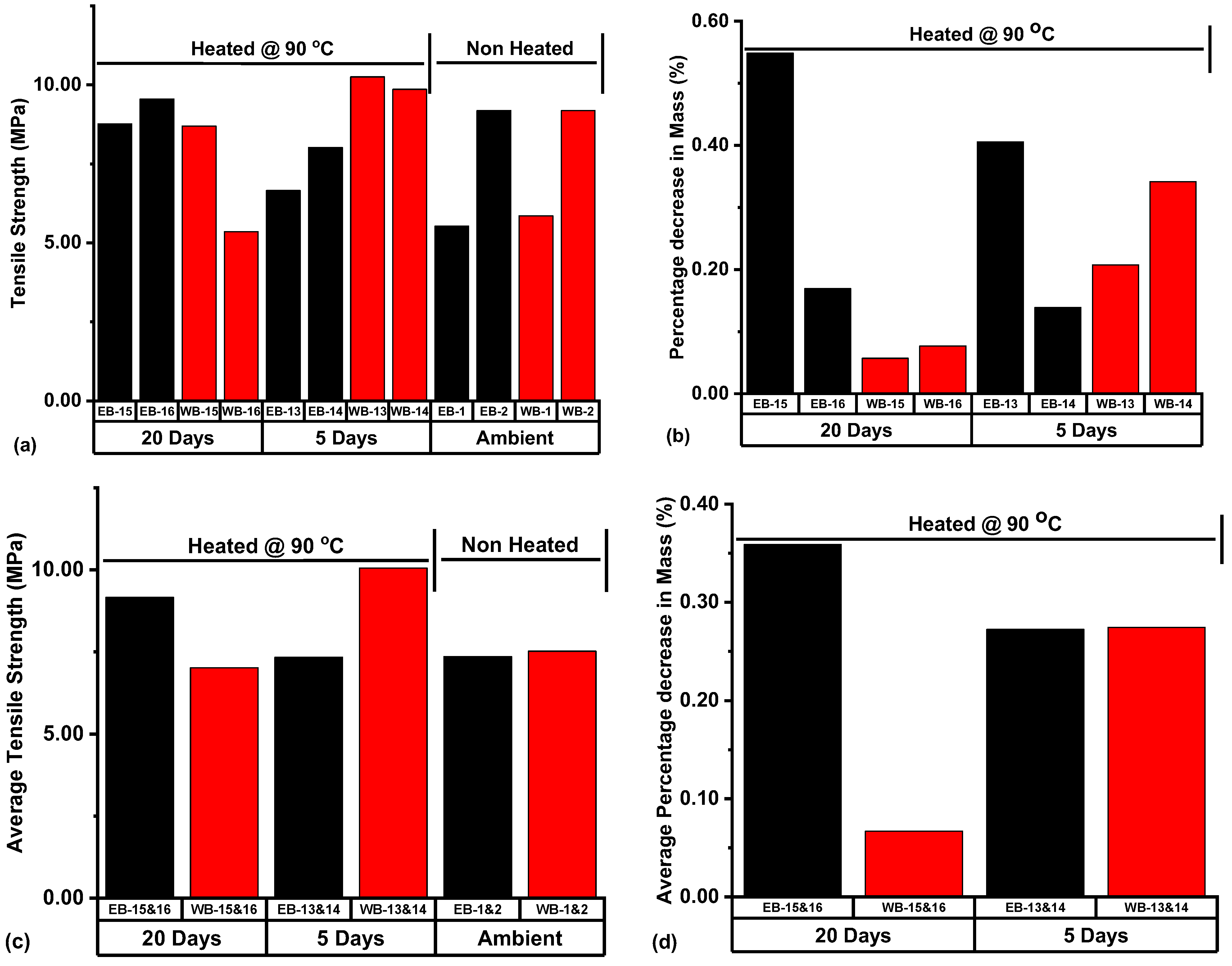
| 21 | EB-13 | Heated at 90 °C for 5 days | 6.66 | SCF + SNCF | Minor fracture at upper section |
| 22 | EB-14 | 8.02 | SCF + SNCF | Non | |
| 23 | WB-13 | 10.25 | SCF + SNCF | Spalling at upper section | |
| 24 | WB-14 | 9.86 | SCF + DNCF | Spalling at sample surface | |
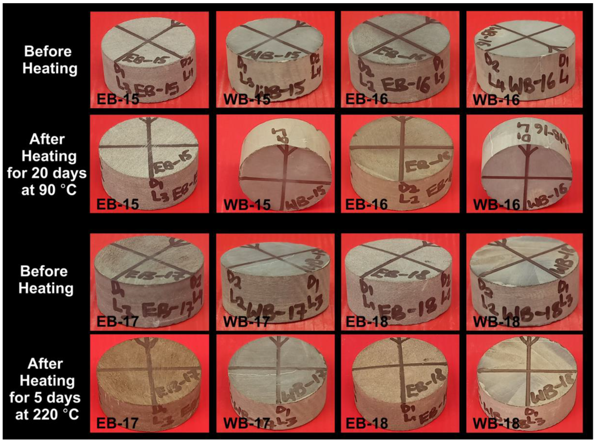
| 25 | EB-15 | Heated at 90 °C for 20 days | 8.77 | SCF + SNCF | Non |
| 26 | EB-16 | 9.55 | SCF + DNCF | Non | |
| 27 | WB-15 | 8.69 | SCF + DNCF | Non | |
| 28 | WB-16 | 5.36 | SCF + SNCF | Non | |
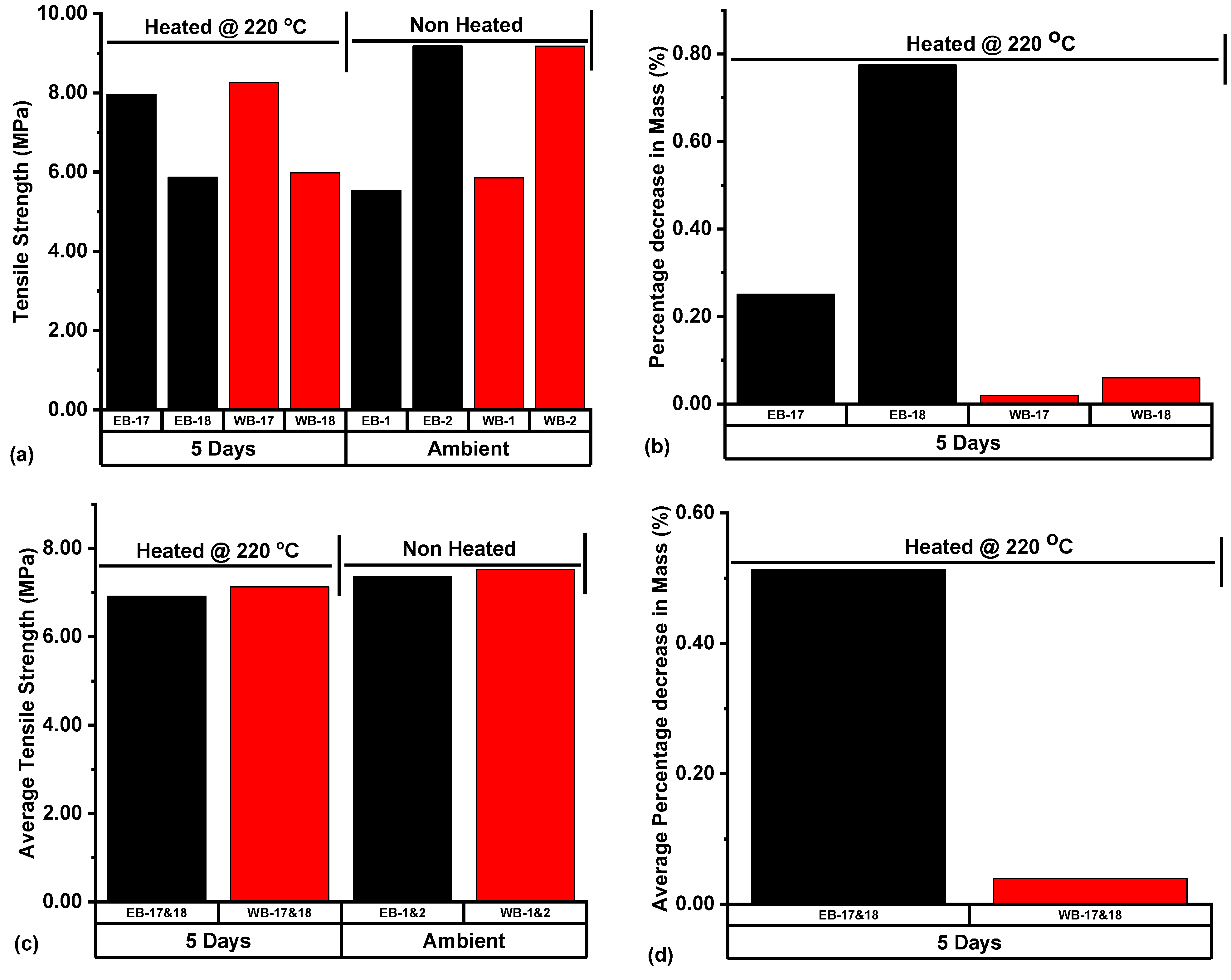
| 29 | EB-17 | Heated at 220 °C for 5 days | 7.95 | SCF + DNCF | Non |
| 30 | EB-18 | 5.87 | SCF | Non | |
| 31 | WB-17 | 8.27 | SNCF + NCAF | Natural crack activation oriented | |
| 32 | WB-18 | 5.98 | SNCF | Thin natural fracture line |
Publisher’s Note: MDPI stays neutral with regard to jurisdictional claims in published maps and institutional affiliations. |
© 2022 by the authors. Licensee MDPI, Basel, Switzerland. This article is an open access article distributed under the terms and conditions of the Creative Commons Attribution (CC BY) license (https://creativecommons.org/licenses/by/4.0/).
Share and Cite
Iferobia, C.C.; Ahmad, M.; Ali, I. Experimental Investigation of Shale Tensile Failure under Thermally Conditioned Linear Fracturing Fluid (LFF) System and Reservoir Temperature Controlled Conditions. Polymers 2022, 14, 2417. https://doi.org/10.3390/polym14122417
Iferobia CC, Ahmad M, Ali I. Experimental Investigation of Shale Tensile Failure under Thermally Conditioned Linear Fracturing Fluid (LFF) System and Reservoir Temperature Controlled Conditions. Polymers. 2022; 14(12):2417. https://doi.org/10.3390/polym14122417
Chicago/Turabian StyleIferobia, Cajetan Chimezie, Maqsood Ahmad, and Imtiaz Ali. 2022. "Experimental Investigation of Shale Tensile Failure under Thermally Conditioned Linear Fracturing Fluid (LFF) System and Reservoir Temperature Controlled Conditions" Polymers 14, no. 12: 2417. https://doi.org/10.3390/polym14122417