
Mechanical Stabilities and Properties of Graphene-like 2D III-Nitrides: A Review


1
Yangtze River Delta Research Institute, Northwestern Polytechnical University, Xi’an 710072, China
2
Physics Department, King Fahd University of Petroleum & Minerals, Dhahran 31261, Saudi Arabia
3
K.A.CARE Energy Research & Innovation Center, Dhahran 31261, Saudi Arabia
4
Interdisciplinary Research Center for Hydrogen and Energy Storage, King Fahd University of Petroleum and Minerals, Dhahran 31261, Saudi Arabia
*
Authors to whom correspondence should be addressed.
Crystals 2023, 13(1), 12; https://doi.org/10.3390/cryst13010012
Submission received: 5 November 2022
/
Revised: 12 December 2022
/
Accepted: 13 December 2022
/
Published: 22 December 2022
(This article belongs to the Section Inorganic Crystalline Materials)
Abstract
:Mechanical stabilities and properties are critical in real applications of materials, as well as material and machine design. With the success of graphene, graphene-like materials arose tremendous interest in the past few years. Different from bulk materials, two-dimensional (2D) materials have prominent non-linear elastic behaviors. Here, we briefly review the mechanical stabilities and properties of graphene-like 2D III-nitrides, including boron nitride (BN), aluminum nitride (AlN), gallium nitride (GaN), indium nitride (InN), and thallium nitride (TlN). These nitrides are excellent wide band gap semiconductors very suitable for modern electronic and optoelectronic applications. As a result, they play a central role in solid-state light-emitting devices. Their Young’s modulus, Poisson’s ratio, ultimate tensile strength, and elastic limits under various strains are extensively studied, as well as their high-order elastic constants and non-linear behaviors. These studies provide a guide for their practical applications and designs.
1. Introduction
The research on 2D nanomaterials with potential next generation electronic device application has seen tremendous progress in the past few years [1,2,3]. Examples of such materials in the nitrides family include graphene-like 2D III-nitrides, including boron nitride (BN), aluminum nitride (AlN), gallium nitride (GaN), indium nitride (InN), and thallium nitride (TlN). We denote them as g-BN, g-AlN, g-GaN, g-InN, and g-TlN throughout this mini review. These nitrides are excellent wide band gap semiconductors very suitable for modern electronic and optoelectronic applications. As a result, they play a central role in the light industry.
There are extensive studies on these materials. For a superlattice sample consisting of an arrangement of six layers of GaN(16 nm)/AlN(13 nm) deposited on top of a 60 nm thick AlN layer grown on a (1–100) SiC substrate, nanobeam electron diffraction analysis results indicate that the strain in the y-direction is equal to zero. In the x-direction, the first 60 nm thick AlN layer appears in a strain state of ~1% compared to the SiC substrate, while the GaN layers are also in tensile strain, but with a much higher strain value of 4.3% [4]. Park et. al reported the formation of intertwined double-spiral few-layer hexagonal BN (h-BN) with the most stable AA′ stacking configuration that is driven by screw dislocations located at the antiphase boundaries of monolayer domains. Moreover, they found that the occurrence of shear strains at the boundaries of merged spiral islands is dependent on the propagation directions of encountering screw dislocations and presented the strained features by density functional theory calculations and atomic image simulations [5]. One previous research indicated that 2D h-BN has high piezoelectric catalytic ability and stability since h-BN can directly convert mechanical energy into chemical energy, which displays the huge potential of two-dimensional piezoelectric materials in relieving energy pressure [6]. Some first-principles calculation results [7] for the semi-hydrogenated-semi-oxidized two-dimensional (111)-oriented bilayer BN nanosheets show that for a few layers, the B (N) atoms of BN nanosheets are more easily bound to H (O), which provides new ideas for achieving high performance BN-based electromagnetic nanodevices. First-principles calculations [8] for the few-layer gallium nitride (GaN) nanosheet presented that with the thickness increases, few-layer GaN nanosheets have suffered from the size-induced transition from indirect semiconductor to metallic as well as from the graphitic planar honeycomb to the wurtzite buckled 2D form, which indicates that there are two competing mechanisms that govern the polarity compensation with the sheet’s net dipole served as an important parameter for determining the sheet’s stable formation. Some first-principles density functional theory calculations for the mechanical and electronic properties of aluminum nitride (AlN) and titanium nitride (TiN) sheets indicate that TiN and AlN layers depending on the atomic configurations and the strain direction can yield remarkable elastic modulus in the range of 137.64 GPa nm for Young’s module and high ultimate tensile strength from 6.29 N/m to around 18.34 N/m [9]. By using ab initio calculations, BN, BP, AlN, and AlP are found to exhibit hyperelastic softening behavior and high inter-atomic rigidity that is highly desirable in the automotive and aeronautical industries [10]. By using MD simulations, Le proposed a formula [11] that can capture the variation of KIc/(σcr1/2) (from 1.87 to 2.45) by considering this dimensionless quantity as a function of the tensile strength-elastic modulus ratio and buckling height-bond length ratio, while molecular mechanics-based models have predicted a constant value of this quantity.
Several experimental and atomistic simulation studies on graphene and carbon nanotubes have proved that 2D nanosheets and nanotubes usually show non-linear elastic deformation during tension up to the intrinsic strength of the material followed by a strain softening up to the fracture [12,13,14,15,16]. To establish a continuum-based framework to capture this non-linear elastic behavior of the 2D nanosheets, the higher-order elastic constants must be considered in the strain energy density function [17,18]. In such a model, the strain energy density is expanded in a Taylor series to include both quadratic as well as higher-order terms in strain. The quadratic term accounts for the linear elastic response of the material while the cubic and higher-order terms account for the strain softening of the elastic stiffness. The higher-order terms can also be used to define other anharmonic properties of this 2D nanostructure including phenomena such as thermal expansion, phonon–phonon interaction, etc. [19].
The goal of this mini-review is to overview and compare the continuum description of the elastic properties of general 2D graphene-like nitrides, including g-BN, g-AlN, g-GaN, g-InN, and g-TlN from ab initio density functional theory calculations via five-order non-linear elasticity (FONE) method. This continuum description is suitable for incorporation into the finite element method. As a result, this method could also be very useful for multiscale calculations passing electronic scale information about mechanical properties to the continuum level. To achieve that, the elastic properties of the monolayer of a graphene-like material were first examined using ab initio density functional theory.
Under the framework of quantum mechanics, the density functional theory (DFT) calculations can predict the elastic properties of materials if one takes into account the structural relaxations along with gradient corrections [20]. It was demonstrated that the resulting continuum description is capable of describing those accompanying ab initio DFT calculations with high accuracy in the infinitesimal strain regime as well as at finite strains, including the strain at the intrinsic stress and beyond in graphene [18]. A higher- rank tensor is associated with each term of the series expansion and the components of the tensor represent the continuum elastic properties. Previous authors had determined the non-zero independent tensor components that correspond to the symmetrical elements of graphene for the second-, third-, fourth- and fifth-order term from stress–strain response of graphene [18]. We extended the method with least-squares solution to over-determined (up to eighth-rank tensor) and well-determined (tenth-rank tensor) linear equations. This method is introduced in the next section and then applied to obtain the continuum description of the elastic properties of monolayer graphene-like materials. The results and analysis are in Section 4, followed by the conclusions.
2. Five-Order Non-Linear Elasticity (FONE) Method
The five-order non-linear elasticity (FONE) method used here is an extension of the method introduced by Wei et al. [18]. The improvement of our work includes the least-squares solution to the over-determined (up to eighth-rank tensor) and well-determined (tenth-rank tensor) linear equations. Take the hexagonal boron nitride monolayer for instance; we used a super cell containing 12 B and 12 N atoms in one plane, with periodic boundary conditions. The undeformed reference configuration is shown in Figure 1, with lattice vectors Hi, I = 1, 2, 3.
FONE is described as follows. When a macroscopically homogeneous deformation (deformation gradient tensor [21] F) is applied, the lattice vectors of the deformed h-BN are hi = FHi. The Lagrangian strain [22] is defined as η = , where I is the identity tensor. The strain energy density has functional form of Φ = Φ(η). The elastic properties of a material are determined from Φ, which is quadratic in strain for a linear elastic material. Non-linear elastic constitutive behavior is established by expanding Φ in a Taylor series in terms of powers of strain η. The symmetric second Piola–Kirchhoff stress tensor, Σij, can be expressed (up to fifth order) as [18]:
where ηij is Lagrangian elastic strain. Summation convention is employed for repeating indices; lower case subscripts range from 1 to 3. Herein, C denotes each higher-order elastic modulus tensor; the rank of each tensor corresponds to the number of subscripts. The second-order elastic constants (SOEC), Cijkl, third-order elastic constants (TOEC), Cijklmn, fourth-order elastic constants (FOEC), Cijklmnop, and fifth-order elastic constants (FFOEC), Cijklmnopqr, are given by the components of the fourth-, sixth-, eighth-, and tenth-rank tensors, respectively.
We used conventional Voigt notation [23] for subscripts: 11→1, 22→2, 33→3, 23→4, 31→5, and 12→6. It should be mentioned that strain η4 = 2η23, η5 = 2η31, η6 = 2η12. Equation (1) can be rewritten as:
where the summation convention for upper case subscripts runs from 1 to 6. These constants are orientation-independent in h-BN due to the six-fold rotation symmetry of the atomic lattice [23]. In this study, we model the monolayer h-BN as a 2D structure and assume that the deformed state of the monolayer h-BN is such that the contribution of bending to the strain energy density is negligible as compared to the in-plane strain contribution. This assumption is reasonable since the radii of curvature of out-of-plane deformation are significantly larger than the in-plane inter-atomic distance. Then, the stress state of monolayer h-BN under those assumptions can be assumed to be 2D and we only consider the in-plane stress and strain components for these kinds of structures. The components of the TOEC, FOEC, and FFOEC tensors can be determined based on the symmetries of the graphene atomic lattice point group D6h which consists of a six-fold rotational axis and six mirror planes as formulated in [18].
The fourteen independent elastic constants of h-BN are determined by a least-squares fit to stress–strain results from ab initio DFT simulations in two steps. In the first step, we use least-squares fit to five stress–strain responses. Five relationships between stress and strain are necessary because there are five independent FFOECs. We obtain the stress–strain relationships by simulating the following deformation states: uniaxial strain in the zigzag direction; uniaxial strain in the armchair direction; and equibiaxial strain. From the first step, we find that the components of SOEC, TOEC, and FOEC are over determined (i.e., the number of linearly independent variables are greater than the number of constraints), and the FFOEC are well determined (the number of linearly independent variables are equal to the number of constrains). Under such circumstances, the second step would be the least-squares solution to these over- and well-determined linear equations.
In the first step, we carried out three deformations: uniaxial strain in the zigzag direction (case z), uniaxial strain in the armchair direction (case a), and equibiaxial strains (case b). For uniaxial strain in the zigzag direction, the strain tensor is:
where ηz is the amount of strain in zigzag direction.
For a given strain tensor, the associated deformation gradient tensor is not unique. The various possible solutions differ from one to another by a rigid rotation. Here, the lack of a one-to-one map relationship between the strain tensor and deformation gradient tensor is not concerned since the calculated energy is invariant under rigid deformation [24,25]. One of the corresponding deformation gradient tensor Fz for uniaxial strain in the zigzag direction is selected as:
where εz is the stretch ratio ε in the zigzag direction. Moreover, ε is determined by the Lagrangian elastic strain in Equation (5):
The stress–strain relationships of the uniaxial strain in the zigzag direction are:
For uniaxial strain in the armchair direction, the strain tensor is:
One of the corresponding deformation gradient tensor Fa for uniaxial strain in the armchair direction is:
where εa is ε in the armchair direction. The stress–strain relationships are:
For equibiaxial strain in-plane, ηa = ηz = η, the strain tensor is:
The corresponding deformation gradient tensor Fb for equibiaxial strain in-plane is:
The stress–strain relationship is:
All fourteen elastic constants contribute to the expressions for stress–strain response for these three deformation states. However, the components of SOEC, TOEC, and FOEC are over determined. As discussed before, we used least-squares solutions to solve the equations A · C = Σ by computing the elastic constants that minimize the Euclidean 2-norm ||Σ − A · C||2. For SOEC components, C11 and C12 are obtained by:
where is the coefficient of the first order of strain in 1 (Equation (9)), and similar notations are used for the others. The Young’s modulus is and Poisson’s ratio is ν = C12/C11.
For TOEC components, C111, C112, and C222 are obtained by:
For FOEC components, C1111, C1112, C1122, and C2222 are obtained by:
For FFOEC components, C11111, C11112, C11122, C12222, and C22222 are obtained by:
With these fourteen independent elastic constants, the continuum formulation of h-BN up to the fifth order can be obtained. FONE provides a continuum formulation, which can present both linear and non-linear elastic mechanical properties. These properties in monolayer h-BN then can be calculated accurately from ab initio DFT calculations. As a result, this FONE method can bridge up the scales in multiscale calculations passing electronic scale information about mechanical properties to the continuum level.
The in-plane stiffness Ys can be obtained from the elastic moduli C11 and C12 as:
Ys = (C112 − C122)/C11.
The Poisson’s ratio ν, which is the ratio of the transverse strain to the axial strain, can be obtained from elastic moduli as:
ν = C11/C12.
With third-order elastic moduli, we can study the effect of pressure on the second-order elastic moduli, where the pressure p acts in the plane of g-AlN. Explicitly, when pressure is applied, the pressure-dependent second-order elastic moduli (, , ) can be obtained from C11, C12, C22, C111, C112, C222, Ys, and n as in Equations (21)–(23).
The velocities of these two types of sound wave are calculated from the second-order elastic moduli and mass density (ρm) using the relationships shown in Equations (24) and (25).
The compressional to shear wave velocity ratio (νp/νs) is a very useful parameter in the determination of a material’s mechanical properties. It depends only on the Poisson’s ratio as shown in Equation (26).
This method is good for general 2D hexagonal structures due to the symmetries. It could be used for monolayer h-BNC heterostructures and other honeycomb-like structures.
3. Density Functional Theory Calculations
In g-BNC materials, the g-BN phase is presented by the hexagonal structure (Figure 1a) of BN locally, which is a six-atom-hexagonal-ring unit and can be denoted as (B3N3). All the “axis 1” (as displayed in Figure 1 and Figure 2) are along the armchair direction (also x direction) and all the “axis 2” are along the zigzag direction (also y direction) in this paper. The g-BN domain in g-BNC hybrid structures is modeled by adjusting the g-BN concentrations in g-BNC while maintaining the integrity of B3N3 within the system. The g-BN domain size in a system can be equivalently expressed by the g-BN concentration in the model as (B3N3)x(C6)1−x, where (C6) denotes the six-atom-hexagonal-ring unit of graphene. The six-atom-hexagonal-ring unit cell is chosen to capture the “soft mode”, which is a particular normal mode exhibiting an anomalous reduction in its characteristic frequency and leading to mechanical instability. This soft mode is a key factor in limiting the strength of monolayer materials and can only be captured in unit cells with hexagonal rings [26]. This g-BNC domain model had been successfully used to study the electronic band structures and linear elastic properties of g-BNC heterostructures in our previous work [27,28].
We considered a conventional unit cell containing six atoms (three metallic atoms and three nitrogen atoms) with periodic boundary conditions for g-AlN (Figure 1b), g-GaN (Figure 1c), and g-TlN (Figure 1d). The 6-atom conventional unit cell was chosen to capture the “soft mode”, which is a particular normal mode exhibiting an anomalous reduction in its characteristic frequency and leading to mechanical instability.
The stress–strain relationship of all these materials under the desired deformation configurations is characterized via first-principles calculations based on density functional theory (DFT). DFT calculations were carried out with the Vienna Ab initio Simulation Package (VASP) [29,30,31,32] which is based on the Kohn–Sham density functional theory (KS-DFT) [33,34] with the generalized gradient approximations as parameterized by Perdew, Burke, and Ernzerhof (PBE) for exchange-correlation functions [35]. For g-BNC, the electrons explicitly included in the calculations are the (2s2p1) electrons of boron, the (2s22p2) electrons of carbon, and the (2s22p3) electrons of nitrogen. For AlN, the electrons explicitly included in the calculations are the (3s23p1) electrons for Al, the (2s22p1) electrons for boron, and the (2s22p3) electrons for nitrogen. For g-GaN, the electrons explicitly included in the calculations are the (2s22p2) electrons for nitrogen atoms and the (3d104s24p1) electrons for gallium atoms. For g-TlN, the electrons explicitly included in the calculations are the 5d106s26p1 electrons for thallium atoms and the 1s22s22p1 electrons for nitrogen atoms. The core electrons are replaced by the projector augmented wave (PAW) approach and pseudo-potential approach [36,37]. A plane-wave cutoff of 520 eV is used for g-BNC and 600 eV is used for g-AlN, g-GaN, g-InN, and g-TlN in all the calculations. The calculations are performed at zero temperature.
The criterion to stop the relaxation of the electronic degrees of freedom is set by requiring the total energy change to be smaller than 10−6 eV. The optimized atomic geometry was achieved through minimizing Hellmann–Feynman forces acting on each atom until the maximum forces on the ions were smaller than 0.001 eV/Å. The atomic structures of all the deformed and undeformed configurations are obtained by fully relaxing an either 24-atom unit cell (g-BNC) or a 6-atom unit cell (other materials) where all atoms are placed in one plane. Periodic boundary conditions are applied for the two in-plane directions.
For g-BNC, the irreducible Brillouin zone was sampled with a Gamma-centered 19 × 19 × 1 k-mesh. Such a large k-mesh was used to reduce the numerical errors caused by the strain of the systems. The initial charge densities were taken as a superposition of atomic charge densities. There was a 14 Å thick vacuum region to reduce the inter-layer interaction to model the single layer system. For g-AlN, the irreducible Brillouin zone was sampled with a C-centered 25 × 25 × 1 k-mesh. There was a 15 Å thick vacuum region to reduce inter-layer interactions to model the single layer system. For g-GeN and g-TlN, the irreducible Brillouin zone was sampled with a Gamma-centered 17 × 17 × 1 k-mesh. There was a 15 Å vacuum region to reduce the inter-layer interaction to model the single layer system. To eliminate the artificial effect of the out-of-plane thickness of the simulation box on the stress, we used the second Piola–Kirchhoff (P–K) stress [38,39] to express the 2D forces per length with units of N/m.
For a general deformation state, the number of independent components of the second-, third-, fourth-, and fifth-order elastic tensors are 21, 56, 126, and 252, respectively. However, there are only fourteen independent elastic constants that need to be explicitly considered due to the symmetries of the atomic lattice point group D6h, which consists of a six-fold rotational axis and six mirror planes [18].
The fourteen independent elastic constants of all these materials are determined by a least-squares fit to the stress–strain results from DFT calculations in two steps, detailed in our previous work [38], which had been well used to explore the mechanical properties of 2D materials [39,40,41,42,43,44,45,46,47,48,49,50,51,52,53,54,55,56,57,58,59,60,61,62,63].
A brief of the FONE method is that, in the first step, we use a least-squares fit of five stress –strain responses. Five relationships between stress and strain are necessary because there are five independent fifth-order elastic constants (FFOEC). We obtain the stress–strain relationships by simulating the following deformation states: uniaxial strain in the zigzag direction (zigzag); uniaxial strain in the armchair direction (armchair); and equibiaxial strain (biaxial). From the first step, the components of the second-order elastic constants (SOEC), the third-order elastic constants (TOEC), and the fourth-order elastic constants (FOEC) are over determined (i.e., the number of linearly independent variables are greater than the number of constrains), and the fifth-order elastic constants are well determined (the number of linearly independent variables are equal to the number of constrains). Under such circumstances, the second step is needed: least-squares solution to these over- and well-determined linear equations.
4. Results and Analysis
4.1. g-BNC
4.1.1. Geometry
The optimized atomistic structures of the five configurations are shown in Figure 2, in ascending order of g-BN concentration as 0% (graphene), 25%, 50%, 75%, and 100% (g-BN). Due to the intrinsic difference between pure g-BN and graphene, the lattice constants of the g-BNC mixtures are obtained by averaging the lattice vectors of the super cells for a direct comparison to pure g-BN and graphene. We found that the lattice constant increases with g-BN concentration x. Our results of the lattice constants are summarized in Table 1, which are in good agreement with experiments on g-BN (2.51 Å) [64] and graphene (2.46 Å) [65]. Regarding the van der Waals corrections, we have extensive investigation on it [66]. We have previously studied the Grimme correction D3 on the high-order elastic constants of hydrogenated graphene [62]. We have concluded that the van der Waals corrections have trivial effect on the high-order elastic constants of the 2D materials. Therefore, the van der Waals corrections should not affect our main results.
When the strains are applied, all the atoms are allowed full freedom of motion. A quasi-Newton algorithm is used to relax all atoms into equilibrium positions within the deformed unit cell that yields the minimum total energy for the imposed strain state of the super cell.
4.1.2. Strain Energy
Both compression and tension are considered with Lagrangian strains ranging from −0.1 to 0.3 with an increment of 0.02 in each step for all three deformation modes. The system’s energy will increase when strains are applied. We define strain energy per atom Es = (Etot − E0)/n, where Etot is the total energy of the strained system, E0 is the total energy of the strain-free system, and n is the number of atoms in the unit cell. This intensive quantity is used for the comparison between different systems. Figure 3 shows the Es as a function of strain in uniaxial armchair, uniaxial zigzag, and equibiaxial deformation.
Es is seen to be anisotropic with strain direction, consistent with the non-isotropic structure of the monolayer g-BNC. Es is non-symmetrical for compression (η < 0) and tension (η > 0) for all three modes. This non-symmetry indicates the anharmonicity of the g-BNC structures. The harmonic region, where the Es is a quadratic function of applied strain, can be taken between −0.02 < η < 0.02. The stresses, derivatives of the strain energies, are linearly increasing with the increase in applied strains in the harmonic region. The anharmonic region is the range of strain where the linear stress–strain relationship is invalid and higher-order terms are not negligible. With an even larger loading of strains, the systems will undergo irreversible structural changes, and the systems are in the plastic region, in which they might fail. The maximum strain before failure is the critical strain. The ultimate strains are determined as the corresponding strain of the ultimate stress, which is the maxima of the stress–strain curve, as discussed in the following section.
4.1.3. Stress–Strain Response
The stress (second P–K stress)–strain (Lagrangian strain) relationship for uniaxial strain in armchair and zigzag directions, as well as equibiaxial strains, are shown in Figure 4. These stress–strain curves reflect the facts of the non-isotropic g-BNC atomic structures, in addition to the anharmonic responses in compression and tension. Overall, stress increases with strain monotonically in all compression cases. The linear relationship between stress and strain is valid in strain from −0.02 to 0.02, which is the linear elastic region.
When the tensile strain is beyond 0.02, a non-linear relationship of stress–strain occurs. There is a maximum stress when tensile strain becomes larger than 0.14 for all five configurations. We denote this maximum stress as ultimate strength and the corresponding strain as ultimate strain. The stress–strain curves of these five configurations are quite similar, due to their similar 2D hexagonal structures. As a consequence, the stress–strain curves overlap. The insets are zoomed in plots showing different mechanical behaviors around the ultimate strains.
Stresses are the derivatives of the strain energies with respect to the strains. The ultimate strength (the maxima in the stress–strain curve) is the maximum stress that a material can withstand while being stretched, and the corresponding strain is the ultimate strain. Under ideal conditions, the critical strain is larger than the ultimate strain. The systems of g-BNC under strains beyond the ultimate strains are in a metastable state, which can be easily destroyed by long wavelength perturbations, vacancy defects, as well as high temperature effects [67]. The ultimate stress and strain are also called ideal stress and strain. The ultimate strain is determined by the intrinsic bonding strength that acts as a lower limit of the critical strain. Thus, it has practical meaning in consideration for its applications.
The ultimate stress and strain of all five configurations at three deformation modes are summarized and plotted in Figure 5, as a function of the g-BN concentrations CBN. Please note that we use CBN instead of x to represent the concentration of the g-BN phase in the rest of the paper. We found that the ultimate strain of a certain configuration is a function of both deformation mode and the directions.
4.1.4. Elastic Constants
The elastic constants are essential to the continuum description of the elastic properties. The continuum responses are the least-squares fit to the stress–strain results from the DFT calculations, as plotted in Figure 6. We then have 20 values for the 14 independent elastic constants of g-BNC from DFT calculations. The fourteen independent elastic constants of g-BNC are determined by least-squares fit to over-determined equations [38]. The results of these fourteen independent elastic constants are grouped in SOEC, TOEC, FOEC, and FFOEC as listed in Table 1.
Due to the symmetry, only C11 and C12 are independent. C11 decreases linearly with respect to CBN, as plotted in the top panel of Figure 6. Our results of Ys, ν from Equations (19) and (20) and elastic constants of the five configurations are shown in bottom panels of Figure 6. Our calculated value of in-plane stiffness of graphene (344.6 N/m) is in good agreement with the experimental value (340 ± 50 N/m) [12] and theoretical predictions (348 N/m [18] and 335 N/m [67]). Our calculated value of g-BN (278.3 N/m) agrees with an ab initio (GGA-PW91) prediction (267 N/m in ref. [67]). Poisson’s ratios ν are 0.18 and 0.23 for graphene and g-BN, in agreement with 0.16 and 0.21, respectively [67]. Our results of Ys, ν, C11, and C12 are also comparable with ab initio predictions [68] and tight-binding calculations [69] of BN nanotubes.
We found that C11 and the in-plane stiffness decrease almost linearly as g-BN concentration increases, while C12, as well as Poisson’s ratio ν, show a rather more complicated behavior (Figure 6). The similar trend of in-plane stiffness and C11 are based on the fact that C11 is dominant, about 6 times bigger than C12. For the same reason, Poisson’s ratio ν has a similar trend as C12. The increment of the Poisson’s ratio with respect to the g-BN concentration indicates a decrement of the network connectivity [70], consistent with the decrement of the density.
The effect of the g-BN concentration on the higher-order elastic constants is shown in Figure 7. In an overview, the third- and fifth-order elastic constants are all negative, in contrast to positive fourth-order elastic constants. From the magnitude, the longitudinal modes (diagonal terms) of elastic constants are much larger than the shear modes (off-diagonal terms) of elastic constants. Comparing the elastic constants in different orders, one can notice that the third-order elastic constants of g-BNC vary mildly with the concentrations of g-BN. However, the fourth- and fifth-order elastic constants have a more complex response to the BN modification.
By considering the variation with respect to the BN concentration, we found that BN modification has a large effect on the longitudinal mode elastic constants but is insensitive to the shear mode elastic constants. For the third-order elastic constants, the longitudinal modes C111 and C222 monotonically increase with respect to the g-BN concentration, opposed to the small wiggles in the curve of shear mode C112. The ratio of C111 to C112 is around 6, the same as the ratio of C11/C12. For the fourth-order elastic constants, the longitudinal modes C1111 and C2222 generally decrease with respect to g-BN concentrations, with disturbances around CBN = 0.5. The shear mode C1122 curve has larger fluctuations than the C1112. For the fifth-order elastic constants, the longitudinal modes C1111 and C2222 are very sensitive to the g-BN concentration, with the minimum at CBN = 0.5. The shear modes C11112, C11122, and C12222 are relatively inert to the g-BN concentration. The valley points of C11111 and C22222 at CBN = 0.5 indicate the instability of g-BNC around CBN = 0.5. This is consistent with our previous observation of bond breaking.
As a comparison of the second-order elastic constants, our results of graphene agree with a previous study of using a 2-atom unit cell [18], as summarized in Table 1. However, there is considerable difference in the higher-order (>2) elastic constants. This is mainly because the primitive unit cell (2-atom unit cell) does not have the freedom to distort along the K1 mode (soft mode) as the primitive translational symmetry is enforced [41]. Such K1 soft mode is a precursor to a phase transition as in soft mode theory or directly leads to mechanical failure. This failure mechanism affects the non-linear behavior of graphene around the ultimate strain, which is characterized by the high-order elastic constants.
The high-order elastic constants are strongly related to anharmonic properties, including thermal expansion, thermos-elastic constants, and thermal conductivity. With higher-order elastic constants, we can easily study the pressure effect on the second-order elastic moduli, generalized Gruneisen parameters, and equations of state. For example, when pressure is applied, the pressure-dependent second-order elastic moduli can be obtained from C11, C12, C22, C111, C112, C222, Ys, and ν [23,38,39,71]. In addition, using the higher- order elastic continuum description, one can obtain the mechanical behaviors under various loading conditions, e.g., under applied stresses rather than strains as demonstrated in a previous study [18]. Furthermore, the high-order elastic constants are important in understanding the non-linear elasticity of materials such as changes in acoustic velocities due to finite strain. As a consequence, nano-devices such as nano surface acoustic wave sensors and nano waveguides could be synthesized by introducing local strain [39].
A good way to check the importance of the high-order elastic constants is to consider the case when they are missing. With the elastic constants, the stress–strain response can be predicted from the elastic theory [38]. We take the configuration of the g-BNC with CBN = 0.25 as an example to demonstrate here. When we only consider the second-order elasticity, the stress varies with strain linearly. As illustrated in Figure 8, the linear behaviors are only valid within a small strain range, about −0.02 ≤ η ≤ 0.02, in the three deformation directions. With the knowledge of the elastic constants up to the third order, the stress–strain curve can be accurately predicted within the range of −0.06 ≤ η ≤ 0.06. Using the elastic constants up to the fourth order, the mechanical behaviors can be well treated up to a strain as large as 0.12. For the strains beyond 0.12, the fifth-order elastic constants are required for an accurate modeling. The analysis of the other configurations comes to the same results.
Our results illustrate that the monatomic layer structures possess different mechanical behaviors in contrast to the bulk or multi-layered structures, where the second-order elastic constants are sufficient in most cases. The second-order elastic constants are relatively easier to calculate from the strain–energy curves [67,72]; however, they are not sufficient. The high-order elastic constants are required for an accurate description of the mechanical behaviors of monatomic layer structures since they are vulnerable to strain due to their geometry confinements.
The g-BNC heterostructures are unstable under large tension. All stress–strain curves in the previous section show that such types of materials will soften when the strain is larger than the ultimate strain. From the viewpoint of chemical bonding, this is due to the bond breaking. This softening behavior is determined by the high-order elastic constants. The high-order elastic constants reflect the high-order non-linear bond strength under large strains. The negative values of FFOECs ensure the softening of materials under large strain beyond ultimate strains. The salient large values of FFOECs of CBN = 0.5 g-BNC structure in Figure 8 make it easier to soften at large strains, indicating less stability.
Our results of mechanical properties of g-BNC are limited to zero temperature due to current DFT calculations. Once the finite temperature is considered, the thermal expansions and dynamics will, in general, reduce the interactions between atoms. As a result, the longitudinal mode elastic constants will decrease with respect to the temperature of the system. The variation of shear mode elastic constants should be more complex in responding to the temperature. A thorough study will be interesting, which is, however, beyond the scope of this study.
4.2. g-AlN
4.2.1. Atomic Structure
We first optimized the equilibrium lattice constant for g-AlN. The total energy as a function of lattice spacing was obtained by specifying nine lattice constants varying from 2.8 Å to 3.4 Å, with full relaxations of all the atoms. A least-squares fit of the energies versus lattice constants with a fourth-order polynomial function yielded the equilibrium lattice constant as a = 3.127 Å, which agrees with previous first-principles calculation results of 3.09 Å [73] and 3.15 Å [74].
The most energetically favorable structure was set as the strain-free structure in this study and the atomic structure, as well as the conventional cell, is shown in Figure 1b. Specifically, the bond length of the Al–N bond is 1.805 Å, which is 0.355 Å (or 25%) longer than the bond length of the B–N bond in g-BN. The N–Al–N and Al–N–Al angles are 120° and all atoms are within one plane. Our resulting atomic structure is in good agreement with previous DFT calculations for pristine g-AlN [73,74] and hydrogen passivated flakes [75,76,77]. The further studies in the following subsections imply that this theoretically predicted structure is mechanically stable.
4.2.2. Strain Energy
When the strains were applied, all the atoms were allowed full freedom of motion. A quasi-Newton algorithm was used to relax all atoms into equilibrium positions within the deformed unit cell that yielded the minimum total energy for the imposed strain state of the super cell.
Both compression and tension were considered with Lagrangian strains ranging from −0.1 to 0.4 with an increment of 0.01 in each step for all three deformation modes. It is important to include the compressive strains since they are believed to be the cause of the rippling of the free-standing atom-thick sheet [78]. It was observed that a graphene sheet experiences biaxial compression after thermal annealing [79], which could also happen with g-AlN. Such an asymmetrical range was chosen due to the non-symmetric mechanical responses of material, as well as its mechanical instability [80], to the compressive and tensile strains.
We define strain energy per atom as Es = (Etot − E0)/n, where Etot is the total energy of the strained system, E0 is the total energy of the strain-free system, and n = 6 is the number of atoms in the unit cell. This size-independent quantity is used for comparison between different systems. Figure 9 shows the Es of g-AlN as a function of strain in uniaxial armchair, uniaxial zigzag, and equibiaxial deformation. Es is seen to be anisotropic with strain direction. Es is non-symmetrical for compression (η < 0) and tension (η > 0) for all three modes. This non-symmetry indicates the anharmonicity of the g-AlN structure.
The harmonic region where the Es is a quadratic function of the applied strain can be observed between −0.02 < η < 0.02. The stresses, which are derivatives of the strain energies, linearly increase with the increase in the applied strains in the harmonic region. The anharmonic region is the range of strain where the linear stress–strain relationship is invalid and higher-order terms are not negligible. With an even larger loading of strain, the system will undergo irreversible structural changes, and the system is then in the plastic region where it may fail. The maximum strain in the anharmonic region is the critical strain. For all three directions, the critical strains are not spotted in the testing range. The ultimate strains are determined as the corresponding strain of the ultimate stress, which is the maximum of the stress–strain curve, as discussed in the following section.
It Is worth noting that, in general, compressive strain will cause buckling of the free-standing thin films, membranes, plates, and nanosheets [78]. The critical compressive strain for buckling instability is much less than the critical tensile strain for fracture, e.g., 0.0001% versus 2% in graphene sheets [80]. However, buckling can be suppressed by applying constraints, such as embedding (0.7%) [81], placing on a substrate (0.4% before heating) [79], thermal cycling on a SiO2 substrate (0.05%) [82] or a BN substrate (0.6%) [83], and sandwiching [84]. Thus, although the buckling relaxation modes are not considered in this study due to the unit cell limit, our study of compressive strains is important in understanding the mechanics of these non-buckling applications.
4.2.3. Stress–Strain Curves
The second P–K stress–Lagrangian strain relationship for uniaxial strains along the armchair and zigzag directions, as well as biaxial strains, are shown in Figure 10. The ultimate strength is the maximum stress that a material can withstand while being stretched, and the corresponding strain is the ultimate strain. Under ideal conditions, the critical strain is larger than the ultimate strain. The systems of perfect g-AlN under strains beyond the ultimate strains are in a metastable state, which can be easily destroyed by long wavelength perturbations, vacancy defects, and high temperature effects [67]. The ultimate strain is determined by the intrinsic bond strength and acts as a lower limit of the critical strain. Thus, it has a practical meaning in consideration of its applications.
The values of the ultimate strengths and strains corresponding to the different strain conditions are summarized in Table 2, compared with those of g-BN, graphene, and graphyne. The material behaves in an asymmetric manner with respect to compressive and tensile strains. With increasing strain, the Al–N bonds are stretched and eventually break. When the strain is applied in the armchair direction, the bonds which are parallel to this direction are more severely stretched than those in other directions. The ultimate strain in armchair deformation is 0.22, larger than that of g-BN, graphene, and graphyne. Under zigzag deformation, in which the strain is applied perpendicular to the armchair direction, there are no bonds parallel to this direction. The bonds inclined to the zigzag direction with an angle of 30° are more severely stretched than those in the armchair direction. The ultimate strain in this zigzag deformation is 0.27, larger than that of g-BN, graphene, and graphyne. At this ultimate strain, the bonds that are at an incline to the armchair direction appear to be broken (middle panel of Figure 10). Under the biaxial deformation, the ultimate strain is ηmb = 0.21, which is smaller than that of g-BN and graphene, but bigger than that of graphyne. As such ultimate strain is applied, all the Al–N bonds are observed to be broken (bottom of Figure 10).
Our results for the positive ultimate strengths as well as the ultimate strains along the three deformation directions imply that the g-AlN structure is mechanically stable. Our result agrees with a previous study of the phonon calculations where imaginary frequencies near the Γ point are absent [73].
It should be noted that the softening of the perfect g-AlN under strains beyond the ultimate strain only occurs under ideal conditions. The systems in these circumstances are in a metastable state, which can be easily destroyed by long wavelength perturbations, vacancy defects, and high temperature effects, and so enter a plastic state [67]. Thus, only the data for strain values lower than the ultimate strain have physical meaning and were used in determining the high-order elastic constants in the following subsection.
Compared to g-BN (right of Figure 10), the stresses in g-AlN respond in a similar fashion to the strain as those in g-BN, but to a much smaller degree. This could be attributed to the weaker chemical bonds in g-AlN than in g-BN.
4.2.4. Elastic Constants
The elastic constants are critical parameters in finite element analysis models for the mechanical properties of materials. Our results for these elastic constants provide an accurate continuum description of the elastic properties of g-AlN from ab initio density functional theory calculations. They are suitable for incorporation into numerical methods such as the finite element technique.
The second-order elastic constants model the linear elastic response. The higher-order (>2) elastic constants are important for characterizing the non-linear elastic response of g-AlN using a continuum description. These can be obtained using a least-squares fit of the DFT data and are reported in Table 3. The corresponding values for graphene are also shown.
We have Ys = 135.7 N m−1 and ν = 0.366 from Equations (19) and (20), which agrees with a previous study [73]. The in-plane stiffness of g-AlN is very small compared to g-BN (49%) and graphene (40%), but comparable to graphyne. The reduction in the in-plane stiffness from g-BN to g-AlN is a result of the weakened Al–N bond compared to the B–N bond in g-BN. All other things being equal, bond length is inversely related to bond strength and the bond dissociation energy, as a stronger bond will be shorter. Considering the bond length, in g-AlN the bond length of Al–N is 1.805 Å, about 25 percent larger than the B–N bond length in g-BN (1.45 Å). The bonds can be viewed as being stretched by the replacement of boron atoms with aluminum atoms with reference to g-BN. These stretched bonds are weaker than the unstretched ones, resulting in a reduction in the mechanical strength.
It is worth noting that our results for the positive second-order elastic constants as well as the in-plane Young’s modulus and Poisso’'s ratio indicate that the g-AlN structure is mechanically stable. This result is consistent with the energy study in the previous section and agrees with a previous study of the phonon calculations where imaginary frequencies near the Γ point are absent [73].
The stress–strain curves in the previous section show that the structure will soften when the strain is larger than the ultimate strain. From the point of view of electron bonding, this is due to the bond weakening and breaking. This softening behavior is determined by the TOECs and FFOECs in the continuum aspect. The negative values of TOECs and FFOECs ensure the softening of the g-AlN monolayer under large strain.
The hydrostatic terms (C11, C22, C111, C222, and so on) of g-AlN monolayers are smaller than those of g-BN and graphene, consistent with the conclusion that the g-AlN is ‘‘softer’’. The shear terms (C12, C112, C1122, etc.) are, in general, smaller than those of g-BN and graphene, which contributes to the high compressibility of g-AlN. Compared to graphene, graphyne, and g-BN, one can conclude that the mechanical behavior of g-AlN is similar to graphyne, and that it is much softer than graphene and g-BN.
The high-order elastic constants are strongly related to the anharmonic properties, including thermal expansion, thermos-elastic constants, and thermal conductivity. With higher-order elastic constants, we can easily study the pressure effect on the second-order elastic moduli, generalized Gruneisen parameters, and equations of state. In addition, using the higher-order elastic continuum description, one can ascertain the mechanical behavior under various loading conditions, e.g., under applied stresses rather than strains as demonstrated in a previous study [18]. Furthermore, the high-order elastic constants are important in understanding the non-linear elasticity of materials such as changes in acoustic velocities due to finite strain.
In order to check the importance of the high-order elastic constants, we consider the case when they are missing. With the elastic constants, the stress–strain response can be predicted from elastic theory [38]. When we only consider the second-order elasticity, the stress varies linearly with strain. Take the biaxial deformation as an example. As illustrated in Figure 11, the linear behaviors are only valid within a small strain range, about −0.02 ≤ η 0.02, the same result as obtained from the energy–strain curves in Figure 9. With knowledge of the elastic constants up to the third order, the stress–strain curve can be accurately predicted within the range of −0.06 ≤ η ≤ 0.06. Using the elastic constants up to the fourth order, the mechanical behavior can be well treated up to a strain as large as 0.12. For strain values beyond 0.12, the fifth-order elastic constant is required for accurate modeling. An analysis of the uniaxial deformations comes to the same results. Further analysis on g-BN (bottom of Figure 11) also confirms the results.
Our results illustrate that the monatomic layer structures possess different mechanical behaviors in contrast to the bulk or multi-layered structures, where the second-order elastic constants are sufficient in most cases. The second-order elastic constants are relatively easy to calculate from the strain–energy curves [67,72]; however, they are not sufficient for monatomic layer structures. The high-order elastic constants are required for an accurate description of the mechanical behavior of monatomic layer structures since they are vulnerable to strain due to their geometry confinements.
Our results for the mechanical properties of g-AlN are limited to zero temperature due to the current DFT calculations. Once a finite temperature is considered, the thermal expansions and dynamics will, in general, reduce the interactions between atoms. As a result, the longitudinal mode elastic constants will decrease with respect to the temperature of the system. The variation of shear mode elastic constants should be more complex in responding to the temperature. A thorough study would be interesting, but is, however, beyond the scope of this study.
4.2.5. Pressure Effect on the Elastic Moduli
The second-order elastic moduli of g-AlN are seen to increase linearly with the applied pressure (Figure 12). However, Poisson’s ratio decreases monotonically with the increase in pressure. C11 is asymmetrical to C22 unlike in the zero-pressure case. C11 = C22 only occurs when the pressure is zero. This anisotropy could be the outcome of anharmonicity.
Compared to g-BN (bottom of Figure 12), the second-order elastic moduli and Poisson’s ratio in g-AlN are more sensitive to the in-plane pressure. This could be attributed to the Al–N bonds being weaker than the B–N bonds.
4.2.6. Pressure Effect on the Velocities of Sound
In the g-AlN monolayer, there are non-zero in-plane Young’s moduli and shear deformations. Hence, it is possible to generate sound waves with different velocities depending on the deformation mode. Sound waves generating biaxial deformations (compressions) are compressional or p-waves. Sound waves generating shear deformations are shear or s-waves. The velocities of these two types of sound wave are calculated from the second-order elastic moduli and mass density (ρm) using the relationships shown in Equations (24) and (25).
The dependence of νp and νs on pressure (biaxial stress) is plotted in Figure 13. The minimum (12 km s−1) of the νp curve occurs at an in-plane pressure of 24 N m−1. However, νs monotonically increases with an increase in pressure. Thus, νp and νs can be tuned by introducing biaxial strain through the stress–strain relationship shown in Figure 10c.
The ratio of νp/νs monotonically decreases with increasing pressure as shown in Figure 13. It converges to a value of 2.0 at positive pressure.
As shown in Figure 13, a sound velocity gradient could be achieved by introducing stress into a g-AlN monolayer. Such a sound velocity gradient could lead to the refraction of sound wavefronts in the direction of lower sound speed, causing the sound rays to follow a curved path [85]. The radius of the curvature of the sound path is inversely proportional to the gradient. In addition, a negative sound speed gradient could be achieved by a negative strain gradient. This tunable sound velocity gradient can be used to form a sound frequency and ranging channel, which is the functional mechanism of waveguides and surface acoustic wave (SAW) sensors [86,87,88]. Compared to g-BN (bottom of Figure 13), the sound velocities in g-AlN are more sensitive to the in-plane pressure. Thus, g-AlN based nano devices for use as SAW sensors, filters, and waveguides may be synthesized using local strains for next generation electronics.
4.3. g-GaN
4.3.1. Atomic Structure
We first optimize the equilibrium lattice constant for g-GaN. The total energy as a function of lattice spacing is obtained by specifying nine lattice constants varying from 2.8 Å to 3.6 Å, with full relaxations of all the atoms. A least-squares fit of the energies versus lattice constants with a fourth-order polynomial function yields the equilibrium lattice constant as a = 3.207 Å. The most energetically favorable structure is set as the strain-free structure in this study and the atomic structure, as well as the conventional cell, is shown in Figure 1c. Specifically, the bond length of Ga–N is 1.852 Å, which is 0.402 Å (or 28%) longer than the bond length of the B–N bond in g-BN. The N–Ga–N and Ga–N–Ga angles are 120° and all atoms are within one plane. Our result for the bond length is in good agreement with a previous first-principles study [73].
4.3.2. Strain Energy
When the strains are applied, all the atoms are allowed full freedom of motion within their plane. A quasi-Newton algorithm is used to relax all atoms into equilibrium positions within the deformed unit cell that yields the minimum total energy for the imposed strain state of the super cell. Both compression and tension are considered with Lagrangian strains ranging from −0.1 to 0.4 with an increment of 0.01 in each step for all three deformation modes. We define strain energy per atom Es = (Etot − E0)/n, where Etot is the total energy of the strained system, E0 is the total energy of the strain-free system, and n = 6 is the number of atoms in the unit cell. This size-independent quantity is used for the comparison between different systems. Figure 14 shows the Es of g-GaN as a function of strain in uniaxial armchair, uniaxial zigzag, and equibiaxial deformation. Es is seen to be anisotropic with strain direction. Es is non-symmetrical for compression (η < 0) and tension (η > 0) for all three modes. This non-symmetry indicates the anharmonicity of the g-GaN structures. The harmonic region where the Es is a quadratic function of applied strain can be taken between −0.02 < η < 0.02. The stresses, derivatives of the strain energies, are linearly increasing with the increase in the applied strains in the harmonic region. The anharmonic region is the range of strain where the linear stress–strain relationship is invalid and higher-order terms are not negligible. With an even larger loading of strains, the systems will undergo irreversible structural changes, and the systems are in a plastic region where they may fail. The maximum strain in the anharmonic region is the critical strain. The critical strains are not spotted in this study. The ultimate strains are determined as the corresponding strain of the ultimate stress, which is the maxima of the stress–strain curve, as discussed in the following section.
4.3.3. Stress–Strain Curves
The second P–K stress–Lagrangian strain relationship for uniaxial strains along the armchair and zigzag directions, as well as biaxial strains, are shown in Figure 15. The stresses are the derivatives of the strain energies with respect to the strains. The ultimate strength is the maximum stress that a material can withstand while being stretched, and the corresponding strain is the ultimate strain. Under ideal conditions, the critical strain is larger than the ultimate strain. The systems of perfect g-GaN under strains beyond the ultimate strains are in a metastable state, which can be easily destroyed by long wavelength perturbations and vacancy defects, as well as high temperature effects [67]. The ultimate strain is determined by the intrinsic bonding strengths and acts as a lower limit of the critical strain. Thus, it has a practical meaning in consideration for its applications.
The ultimate strengths and strains corresponding to the different strain conditions are summarized in Table 2, compared with that of g-BN and graphene. The material behaves in an asymmetric manner with respect to compressive and tensile strains. With increasing strains, the Ga–N bonds are stretched and eventually rupture. When the strain is applied in the armchair direction, the bonds which are parallel to this direction are more severely stretched than those in other directions. The ultimate strain in armchair deformation is 0.18 (top panel of Figure 15), smaller than that of g-BN and graphene. Under the zigzag deformation, in which the strain is applied perpendicular to the armchair, there is no bond parallel to this direction. The bonds at an incline to the zigzag direction with an angle of 30° are more severely stretched than those in the armchair direction. The ultimate strain in this zigzag deformation is 0.22, smaller than that of g-BN and graphene. At this ultimate strain, the bonds that are at an incline to the armchair direction appear to be ruptured (middle panel of Figure 15). Under the biaxial deformation, the ultimate strain is ηmb = 0.16, which is the smallest among those of the three compared. As the ultimate strain is applied, all the Ga–N bonds are observed to be ruptured (bottom of Figure 15).
It should be noted that the softening of the perfect g-GaN under strains beyond the ultimate strains only occurs for ideal conditions. The systems under this circumstance are in a metastable state, which can be easily destroyed by long wavelength perturbations and vacancy defects, as well as high temperature effects, and enter a plastic state [67]. Thus, only the data within the ultimate strain have physical meaning and were used in determining the high-order elastic constants in the following subsection.
4.3.4. Elastic Constants
The elastic constants are critical parameters in finite element analysis models for mechanical properties of materials. Our results of these elastic constants provide an accurate continuum description of the elastic properties of g-GaN from ab initio density functional theory calculations. They are suitable for incorporation into numerical methods such as the finite element technique.
The second-order elastic constants model the linear elastic response. The higher-order (>2) elastic constants are important to characterize the non-linear elastic response of g-GaN using a continuum description. These can be obtained using least-squares fit of the DFT data and are reported in Table 3. Corresponding values for graphene are also shown. We have Ys = 109.4 (N/m) and ν = 0.431 from Equations (19) and (20), in good agreement with a previous study, which has Ys = 110 (N/m) and ν = 0.48 [73]. The in-plane stiffness of g-GaN is very small compared to g-BN (39%) and graphene (32%). The reduction in the in-plane stiffness from g-BN to g-GaN is a result of the weakened bond of Ga-N compared to the B-N bond in g-BN. With all other things being equal, bond length is inversely related to bond strength and the bond dissociation energy, as a stronger bond will be shorter. Considering the bond length, in g-GaN the bond length of Ga-N is 1.852 Å, about 28% larger than the B–N bond length in g-BN (1.45 Å). The bonds can be viewed as being prior stretched by the replacement of boron atoms with gallium atoms, in reference to g-BN. These stretched bonds are weaker than those unstretched, resulting in a reduction in the mechanical strength.
Knowledge of higher-order elastic constants is very useful in understanding anharmonicity. Using the higher-order elastic continuum description, one can calculate the stress and deformation state under uniaxial stress, rather than uniaxial strain [18]. Explicitly, when pressure is applied, the pressure-dependent second-order elastic moduli can be obtained from the high-order elastic continuum description [23,27,39,71]. The third-order elastic constants are important in understanding the non-linear elasticity of materials such as changes in acoustic velocities due to finite strain. Therefore, nanodevices such as nano surface acoustic wave sensors and nano waveguides could be synthesized by introducing local strain [28,39].
It is worthy to note that the uncertainty of the high-order elastic constants arises from the propagation of the numerical error of the total energy calculations. The constringency of the total energy is 10−6 eV. The uncertainty of the second-, third-, fourth-, and fifth-order elastic constants are 10−2, 100, 102, and 104, respectively.
Stress–strain curves in the previous section show that they will soften when the strain is larger than the ultimate strain. From the point of view of electron bonding, this is due to the bond weakening and breaking. This softening behavior is determined by the TOECs and FFOECs in the continuum aspect. The negative values of TOECs and FFOECs ensure the softening of the g-GaN monolayer under large strain.
The hydrostatic terms (C11, C22, C111, C222, and so on) of g-GaN monolayers are smaller than those of g-BN and graphene, consistent with the conclusion that the g-GaN is “softer.” The shear terms (C12, C112, C1122, etc.), in general, are smaller than those of g-BN and graphene, which contributes to the high compressibility of g-GaN. Compared to graphene and g-BN, one can conclude that the mechanical behavior of g-GaN is much softer than graphene and g-BN.
4.3.5. Effect of Pressure on the Elastic Moduli
With third-order elastic moduli, we can study the effect of pressure on the second-order elastic moduli, where the pressure p acts in the plane of g-GaN. Explicitly, when pressure is applied, the pressure-dependent second-order elastic moduli (, , ) can be obtained from C11, C12, C22, C111, C112, C222, Ys, and ν as in Equations (21)–(23).
The second-order elastic moduli of g-GaN are seen to increase linearly with the applied pressure (Figure 16). However, Poisson’s ratio decreases monotonically with the increase in pressure. is asymmetrical to , unlike the zero-pressure case. = = C11 only occurs when the pressure is zero. This anisotropy could be the outcome of anharmonicity.
4.3.6. Promising Applications
In the g-GaN monolayer, there are non-zero in-plane Young’s moduli and shear deformations. Hence, it is possible to generate sound waves with different velocities depending on the deformation mode. Sound waves generating biaxial deformations (compressions) are compressional or p-waves. Sound waves generating shear deformations are shear or s-waves. The sound velocities of these two types of waves are calculated from the second-order elastic moduli and mass density using the relationships shown in Equations (24) and (25).
The dependence of vp and vs on pressure (biaxial stress) is plotted in Figure 17. The minimum (10 km/s) of the vp curve occurs at an in-plane pressure of 1 N/m. However, vs monotonically increases with an increase in pressure. Thus, they can be tuned by introducing the biaxial strain through the stress–strain relationship shown in Figure 15c.
The compressional to shear wave velocity ratio (vp/vs) is a very useful parameter in the determination of a material’s mechanical properties. It depends only on the Poisson’s ratio as in Equation (26). The ratio of vp/vs monotonically decreases with an increase in pressure as shown in Figure 17. It tends to approach a value of 2.0 at positive pressure.
Notice that a sound velocity gradient could be achieved by introducing stress into g-GaN, which could lead to refraction of sound wavefronts in the direction of lower sound speed, causing the sound vectors to follow a curved path [85]. The radius of curvature of the sound path is inversely proportional to the gradient. Additionally, a negative sound speed gradient could be achieved by a negative strain gradient. This tunable sound velocity gradient can be used to form a sound frequency and ranging channel, which is the functional mechanism of waveguides and surface acoustic wave (SAW) sensors [87,88]. Thus, g-GaN-based nanodevices of SAW sensors, filters, and waveguides may be synthesized using local strains for next generation electronics.
4.4. g-InN
4.4.1. Atomic Structure
We first optimize the atomistic structures for g-InN monolayers. The initial configuration is generated by placing 3 indium atoms and 3 nitrogen atoms alternatively on the same plane, forming the 6-atom unit cell. The relaxed structure shows that the six atoms are still coplanar. The most energetically favorable structure was set as the strain-free structure in this study and the atomic structure, as well as the conventional cell, is shown in Figure 1b. Specifically, the bond length of the In–N bond is 2.074 Å, which is 0.554 Å (or 36.45%) longer than the bond length of the B–N bond in g-BN. The N–In–N and In–N–In angles are 120°. The lattice constant or the second nearest neighbor distance is 3.585 Å. Our results agree with a previous DFT study [89]. It is worth noting that the lattice constants of Wurtzite structure of bulk InN are a = 3.540 and c = 5.704 Å in experimental measurement [90]. This strain-free structure is then set as the reference when mechanical strain is loaded.
4.4.2. Strain Energy
When strain is applied, the system will be disturbed away from the equilibrium state. All the atoms of the system are allowed full freedom of motion. A quasi-Newton algorithm is used to relax all atoms into equilibrium positions within the deformed unit cell that yields the minimum total energy for the imposed strain state of the super cell. Since the configuration energy of the strain-free configuration is the minimum of the potential well, any strain will increase the system’s energy. By applying different amounts of strain in different directions, the potential well can be explored.
Lagrangian strains ranging from −0.1 to 0.3 are considered with an increment of 0.01 in each step for all three deformation modes. It is important to include the compressive strains since they are believed to be the cause of the rippling of the free-standing atomic sheet [19]. Because it was reported that a graphene sheet experiences biaxial compression after thermal annealing [91], this could also happen with g-InN monolayers. We selected such an asymmetrical strain range (−0.1 ≤ ƞ ≤ 0.3) owing to the non-symmetric mechanical responses of material. The lower and upper boundary of the strain are consequent upon its mechanical instability to the compressive and tensile strains.
We define strain energy per atom as Es = (Etot − E0)/n, where Etot is the total energy of the strained system, E0 is the total energy of the strain-free system, and n = 6 is the number of atoms in the unit cell. This size-independent quantity is used for comparison between different systems. Figure 18a shows the Es of g-InN as a function of strain in uniaxial armchair, uniaxial zigzag, and equibiaxial deformation. Es is seen to be anisotropic with strain direction. Es is non-symmetrical for compression (η < 0) and tension (η > 0) for all three modes. This non-symmetry indicates the anharmonicity of the g-InN structure. It is worth noting that for small strains, there is a harmonic region, where the Es is a quadratic function of applied strain. Therefore, the stresses as the derivatives of the strain energies are linearly increasing with the increase in the applied strains in the harmonic region. From the plots of the strain energy profile, one can tell that the harmonic region can be taken between −0.02 < η < 0.02 in the g-InN monolayers.
When the strain is larger, the linear stress–strain relationship is invalid. The range of these strains is an anharmonic region. The main feature of the anharmonic region is that the higher-order terms are not negligible. With an even larger loading of strains, the systems will undergo irreversible structural changes. Then, the system enters a plastic region where it may fail into parts. The maximum strain in the anharmonic region is the ultimate strain. The summation of the critical tensile strain and critical compressive strain is the stable region of that deformation. The width of the stable region defines the opening width of the potential energy well (Figure 18). In general, the opening width and depth of the potential energy wells reflect the flexibility and strength of a nanostructure, respectively. The average width of the stable regions of the three deformation modes (i.e., the opening width of the potential energy wells) is a reasonably good scale for the mechanical stabilities of the nanostructures. As a result, from the point view of potential energy, we conclude that g-InN is mechanically stable. However, it is less stable than g-BN, because both the depth and width of the potential energy well are smaller than that of g-BN. Besides the scale for the mechanical stabilities, strain energy profile can be used to estimate the range of lattice mismatch feasible for epitaxial growth of the 2D materials on the substrates [92].
4.4.3. Stress–Strain Curves
We plot the stress–strain relationship in Figure 19 along the three modes of uniaxial strains along the armchair direction (mode a), uniaxial strains along the zigzag direction (mode z), and biaxial strains (mode b). The material behaves in an asymmetric manner with respect to compressive and tensile strains. With increasing strains, the In–N bonds are stretched and eventually rupture. When strain is applied in mode a, the bonds of those parallel in this direction are more severely stretched than those in other directions. Under the deformation mode z, in which the strain is applied perpendicularly to the armchair direction, there is no bond parallel to this direction. The two In–N bonds at an incline to the zigzag direction with an angle of about 30°are more severely stretched than those in the armchair direction. Under the ultimate strain in mode z, which is 0.26, the two In–N bonds that are at an incline to the armchair direction are observed to rupture. Under the ultimate strain in mode b, ηub = 0.18, the two In–N bonds that are at an incline to the zigzag direction with an angle of about 30° are observed to rupture.
4.4.4. Elastic Constants
The elastic constants are essential parameters to describe the elasticity of materials. The 14 independent elastic constants of g-InN are determined by a least-squares fit to the stress–strain results from DFT calculations [38]. The second-order elastic constants model the linear elastic response. The higher-order (>2) elastic constants are important to characterize the non-linear elastic response of g-InN using a continuum description. These can be obtained using the least-squares fit of the DFT data and are reported in Table 1. Corresponding values for graphene are also shown.
Our result of the in-plane stiffness of g-InN is Ys = 62.0 N/m, much smaller than that of g-BN and graphene. In order to interpolate our results in terms of standard units of gPa, we need the size of the out-of-plane dimension, which, however, is not well defined in 2D material. Taking the inter-layer vdW distance of 5.7 Å from its 3D layered Wurtzite-type structure [90], our result of the in-plane stiffness is 109 gPa, less than the bulk modulus (125 gPa) of its bulk counterpart [90]. This could be a consequence of the stretch of its lattice constants. The Poisson’s ratio of g-InN is ν = 0.586, about 2.6 and 3.3 times that of g-BN and graphene, respectively.
Higher-order (>2) elastic constants are important quantities [19] in studying the non-linear elasticity, harmonic generation, lattice defects, phase transitions, strain softening, temperature dependence of elastic constants, phonon–phonon interactions, photon–phonon interactions, thermal expansion (through the Gruneisen parameter), echo phenomena, and so on [43]. Experimentally, the higher-order elastic constants can be determined by measuring the changes of sound velocities under the application of hydrostatic and uniaxial stresses [91]. As it is more convenient to apply pressure in experiments, the full stress–strain relationship described by the higher-order elastic constants are critical. Explicitly, when pressure is applied, the pressure-dependent second-order elastic moduli can be obtained from the higher-order elastic continuum description [38]. The third-order elastic constants are important in understanding the non-linear elasticity of materials, such as changes in acoustic velocities due to finite strain. As a consequence, nanodevices (such as nano surface acoustic wave sensors and nano waveguides) could be synthesized by introducing local strain [28,39].
These 14 components of the elastic constants in FONE are summarized in Table 3. The normal terms are in charge of the strength of the material, and the shear terms reflect more about the flexibility. The comparison of the data in Table 3 reveals that the normal terms of g-InN monolayers are smaller in magnitude than those of g-BN and graphene, consistent with the conclusion that the g-InN is “softer”. However, the shear terms do not show a clear trend. The g-InN monolayers exhibit instability under large tension. Stress–strain curves in the previous section show that they might soften when the strain is larger than the ultimate strain. From the point of view of electron bonding, this is due to the bond weakening and breaking. This softening behavior is determined by the TOECs and FFOECs in the continuum aspect. The negative values of TOECs and FFOECs ensure the softening of g-InN monolayer under large strain. It should be pointed out that the tensile strength could be an overestimate of the onset of the instability due to the limitation of the model [93].
The importance of the high-order elastic constants can be perceived when we consider their contribution to the non-linear elasticity. When we only consider the second-order elasticity, the stress varies with strain linearly. Take the biaxial deformation as an example. As illustrated in Figure 20, the linear behaviors are only valid within a small strain range, about 0.02, ηh = 0.02. With the knowledge of the elastic constants up to the third order, the stress–strain curve can be accurately predicted within the range of η ≤ 0.06. Using the elastic constants up to the fourth order, the mechanical behaviors can be well treated up to a strain as large as 0.1. For the strains beyond 0.1, the fifth-order elastic constants are required for accurate modeling. The analysis of the uniaxial deformations provides similar results.
4.4.5. Pressure Effect on the Elastic Moduli
As a demonstration of the usage of the high-order elastic constants, we predicted the pressure effect on the elastic moduli from these elastic constants (Table 3). The pressure effect on the photoluminescence and emission energies of the InN/GaN super lattices has been reported [94]. The non-linear elasticity and the pressure dependence of elastic constants have been investigated in bulk III-N compounds [95]. However, the pressure effect on the elastic moduli is still unknown in g-InN monolayers. We calculate the effect of the second-order elastic moduli on the pressure p acting in the plane of g-InN from the third-order elastic moduli. Explicitly, when pressure is applied, the pressure-dependent second-order elastic moduli can be obtained from the high-order elastic continuum description [28].
The second-order elastic moduli (, , ) can be obtained from C11, C12, C22, C111, C112, C222, Ys, and υ, as detailed inelastic moduli of g-InN are seen to increase linearly with the applied pressure (Figure 21). Poisson’s ratio also increases monotonically with increasing pressure. is not symmetrical to anymore; only when P = 0, = = C11. This anisotropy could be the outcome of anharmonicity.
4.4.6. Mechanical Instabilities
Mechanical instabilities are the most important in real applications and material or system designs. The ultimate strains are determined as the corresponding strain of the ultimate stress, which is the maxima of the stress–strain curve. The ultimate strengths and strains corresponding to the different strain conditions are summarized in Table 2, compared with that of g-BN and graphene, since they have similar structures, and they are close to each other in the periodic table. The g-InN sheet behaves in an asymmetric manner with respect to compressive and tensile strains. With increasing strains, the B–B bonds are stretched and eventually rupture. The positive slopes of the stress–strain curves and the positive ultimate tensile stresses indicate that this structure is mechanically stable.
The g-InN sheet behaves in an asymmetric manner with respect to compressive and tensile strains. With increasing strains, the In–N bonds are stretched and eventually rupture. The positive slope of the stress–strain curves and the positive ultimate tensile stresses indicate that this structure is mechanically stable. Our results show that the g-InN monolayers are stable under various strains. From the view of energy, the mechanical instabilities are related to the energy barriers, over which the material fails. In our ideal model, this energy barrier is the binding energy. Therefore, we can estimate the binding energy of 1.3 eV from the strain-energy plot (Figure 18) with ηmb = 0.15. Note that the softening of the g-InN monolayers under strains beyond the ultimate strains only occurs for ideal conditions. The systems under this circumstance are in a metastable state, which can be easily destroyed by long wavelength perturbations and vacancy defects, as well as high temperature effects, and enter a plastic state [67]. Thus, only the data within the ultimate strain have physical meaning.
4.5. g-TlN
4.5.1. Atomic Structure
We first optimize the equilibrium lattice constant for g-TlN. The total energy as a function of lattice spacing is obtained by specifying nine lattice constants varying from 3.3 Å to 4.1 Å, with full relaxations of all the atoms. A least-squares fit of the energies versus lattice constants with a fourth-order polynomial function yields the equilibrium lattice constant as a = 3.731 Å. The most energetically favorable structure is set as the strain-free structure in this study and the atomic structure, as well as the conventional cell, is shown in Figure 1d. Specifically, the bond length of Tl–N bond is 2.154 Å, which is 0.704 Å (or 49%) longer than the bond length of B–N bond in g-BN. The N–Tl–N and Tl–N–Tl angles are 120° and all atoms are within one plane. Our result of bond length is in good agreement with previous DFT calculations of N12Tl12H12.
4.5.2. Strain Energy
When the strains are applied, all the atoms are allowed full freedom of motion within their plane. A quasi-Newton algorithm is used to relax all atoms into equilibrium positions within the deformed unit cell that yields the minimum total energy for the imposed strain state of the super cell.
Both compression and tension are considered with Lagrangian strains ranging from −0.1 to 0.3 with an increment of 0.01 in each step for all three deformation modes. We define strain energy per atom Es = (Etot − E0)/n, where Etot is the total energy of the strained system, E0 is the total energy of the strain-free system, and n = 6 is the number of atoms in the unit cell. This size-independent quantity is used for the comparison between different systems. Figure 22 shows the Es of g-TlN as a function of strain in uniaxial armchair, uniaxial zigzag, and biaxial deformation. Es is seen to be anisotropic with strain direction. Es is non-symmetrical for compression (η < 0) and tension (η > 0) for all three modes. This non-symmetry indicates the anharmonicity of the g-TlN structures. The harmonic region where the Es is a quadratic function of applied strain can be taken between −0.02 < η < 0.02. The stresses, derivatives of the strain energies, are linearly increasing with the increase in the applied strains in the harmonic region. The anharmonic region is the range of strain where the linear stress–strain relationship is in-valid and higher-order terms are not negligible. With an even larger loading of strains, the systems will undergo irreversible structural changes, and the systems are in a plastic region where they may fail. The maximum strain in the anharmonic region is the critical strain. The critical strain is 0.2 under armchair deformation. However, for the other two directions, the critical strains are not spotted. The ultimate strains are determined as the corresponding strain of the ultimate stress, which is the maxima of the stress–strain curve, as discussed in the following section.
4.5.3. Stress–Strain Curves
The second P–K stress–Lagrangian strain relationship for uniaxial strains along the armchair and zigzag directions, as well as biaxial strains are shown in Figure 19. The ultimate strength is the maximum stress that a material can withstand while being stretched, and the corresponding strain is the ultimate strain. Under ideal conditions, the critical strain is larger than the ultimate strain. The systems of perfect g-TlN under strains beyond the ultimate strains are in a metastable state, which can be easily destroyed by long wavelength perturbations, vacancy defects, as well as high temperature effects [67]. The ultimate strain is determined by the intrinsic bonding strengths and acts as a lower limit of the critical strain. Thus, it has a practical meaning in considering its applications.
The ultimate strengths and strains corresponding to the different strain conditions are summarized in Table 2, compared with that of g-BN, graphene, and graphyne. The material behaves in an asymmetric manner with respect to compressive and tensile strains. With increasing strains, the Tl–N bonds are stretched and eventually rupture. When the strain is applied in the armchair direction, the bonds of those parallel with this direction are more severely stretched than those in other directions. The ultimate strain in armchair deformation is 0.17, smaller than that of g-BN, graphene, and graphyne. The critical strain is 0.2 under armchair deformation, where there is big drop of the stresses (top panel of Figure 23), indicating the failure of the system. However, for the other two directions, the critical strains are not spotted. Under the zigzag deformation, in which the strain is applied perpendicular to the armchair, there is no bond parallel to this direction. The bonds incline to the zigzag direction with an angle of 30° are more severely stretched than those in the armchair direction. The ultimate strain in this zigzag deformation is 0.21, smaller than that of g-BN and graphene, while the same as graphyne. At this ultimate strain, the bonds that are at an incline to the armchair direction appear to be ruptured (middle panel of Figure 23). Under the biaxial deformation, the ultimate strain is bm = 0.16, which is the smallest among those of g-BN, graphene, and graphene. As such ultimate strain applied, all the Tl–N bonds are observed to be ruptured (bottom panel of Figure 23).
It should be noted that the softening of the perfect g-TlN under strains beyond the ultimate strains only occurs for ideal conditions. The systems under this circumstance are in a metastable state, which can be easily destroyed by long wavelength perturbations and vacancy defects, as well as high temperature effects, and enter a plastic state [67]. Thus, only the data within the ultimate strain have physical meaning and was used in determining the high-order elastic constants in the following subsection.
4.5.4. Elastic Constants
The elastic constants are critical parameters in finite element analysis models for mechanical properties of materials. Our results of these elastic constants provide an accurate continuum description of the elastic properties of g-TlN from ab initio density functional theory calculations. They are suitable for incorporation into numerical methods such as the finite element technique.
The second-order elastic constants model the linear elastic response. The higher-order (>2) elastic constants are important to characterize the non-linear elastic response of g-TlN using a continuum description. These can be obtained using the least-squares fit of the DFT data and are reported in Table 3. Corresponding values for graphene are also shown.
The in-plane stiffness of g-TlN is very small compared to g-BN (12%), graphene (10%), and graphyne (21%). The reduction in the in-plane stiffness from g-BN to g-TlN is a result of the weakened bond of Tl–N compared to the B–N bond in g-BN. While all other things are equal, bond length is inversely related to bond strength and the bond dissociation energy, as a stronger bond will be shorter. Considering the bond length, in g-TlN the bond length of Tl–N is 2.154 Å, about 49 percent larger than B–N bond length in g-BN (1.45 Å). The bonds can be viewed as being stretched prior by the introduction of thallium atoms, in reference to g-BN. Stretched bonds are weaker than those unstretched, leading to a reduction in the mechanical strength.
Using the higher-order elastic continuum description, one can calculate the stress and deformation state under uniaxial stress, rather than uniaxial strain [18]. Explicitly, when pressure is applied, the pressure-dependent second-order elastic moduli can be obtained from the high-order elastic continuum description [23,27,39,71]. The third-order elastic constants are important in understanding the non-linear elasticity of materials such as changes in acoustic velocities due to finite strain. Therefore, nano-devices such as nano surface acoustic wave sensors and nano waveguides could be synthesized by introducing local strain [28,39].
Stress–strain curves in the previous section show that they will soften when the strain is larger than the ultimate strain. From the point of view of electron bonding, this is due to the bond weakening and breaking. This softening behavior is determined by the TOECs and FFOECs in the continuum aspect. The negative values of TOECs and FFOECs ensure the softening of g-TlN monolayer under large strain.
The hydrostatic terms (C11, C22, C111, C222, and so on) of g-TlN monolayers are smaller than those of g-BN and graphene, consistent with the conclusion that the g-TlN is “softer”. The shear terms (C12, C112, C1122, etc.), in general, are smaller than those of g-BN and graphene, which contributes to its high compressibility. Compared to graphene, graphyne, and g-BN, one can conclude that the mechanical behavior of g-TlN is similar to graphyne, and much softer than graphene and g-BN.
4.5.5. Pressure Effect on the Elastic Moduli
With third-order elastic moduli, we can study the effect of the second-order elastic moduli on the pressure P acting in the plane of g-TlN. Explicitly, when pressure is applied, the pressure-dependent second-order elastic moduli (, , ) can be obtained from C11, C12, C22, C111, C112, C22, Ys, and ν as in Equations (21)–(23).
The second-order elastic moduli of g-TlN are seen to increase linearly with the applied pressure (Figure 24). However, Poisson’s ratio decreases monotonically with the increase in pressure. is asymmetrical to unlike the zero-pressure case. = = C11 only occurs when the pressure is zero. This anisotropy could be the outcome of anharmonicity.
5. Discussion
The benefits and challenges for graphene-like materials to form next generation electronics are widely discussed, and research topics cover self-heating issues [96] and cooling strategies for next generation high-power electronic devices [97,98,99,100,101,102]. This section, on the other hand, focuses on the comparison of mechanical properties of graphene structures. We studied the mechanical stability and properties of g-XN materials, where X is an element from the boron family, under various strains using DFT-based first-principles calculations. We also calculated the mechanical properties of g-BN in the same environment for a direct comparison. All calculated parameters are listed in Table 2 and Table 3.
For g-AlN, it is observed it exhibits a non-linear elastic deformation up to an ultimate strain, which is 0.22, 0.27, and 0.21 for armchair, zigzag, and biaxial directions, respectively. The deformation and failure behavior and the ultimate strength are anisotropic. It has a relatively low in-plane stiffness (135.7 N m21) and a large Poisson’s ratio compared to g-BN and graphene. Compared to g-BN, g-AlN has 49% in-plane stiffness, 67%, 60%, and 53% ultimate strengths in armchair, zigzag, and biaxial strains, respectively, and a Poisson’s ratio 1.6 times larger. It was found that g-AlN can sustain larger uniaxial and smaller biaxial strain before it ruptures.
The non-linear elasticity of g-AlN was investigated. We found an accurate continuum description of the elastic properties of g-AlN by explicitly determining the fourteen independent components of the high-order (up to fifth order) elastic constants from the fitting of the stress–strain curves obtained from DFT calculations. These data are useful to develop a continuum description which is suitable for incorporation into a finite element analysis model for g-AlN’s applications at a large scale. We also find that the harmonic elastic constants are only valid within a small range of -.02 ≤ η ≤ 0.02. With the knowledge of the elastic constants up to the third order, the stress–strain curve can be accurately predicted within the range of −0.06 ≤ η ≤ 0.06. Using the elastic constants up to the fourth order, the mechanical behavior can be accurately predicted up to a strain as large as 0.12. For the strains beyond 0.12, the fifth-order elastic constants are required for accurate modeling. The high-order elastic constants reflect the high-order non-linear bond strength under large strains.
The second-order elastic constants including the in-plane stiffness are predicted to monotonically increase with pressure while Poisson’s ratio monotonically decreases with increasing pressure. The sound velocity of a compressional wave has a minimum at an in-plane pressure of −4 N m−1 while that of the shear wave monotonically increases with pressure. The ratio of νp/νs monotonically decreases with the increase in pressure and converges to a value of 2.0 at positive pressure. Our results of the positive ultimate strengths and strains, second-order elastic constants, and the in-plane Young’s modulus indicate that the graphene-like structure of hexagonal AlN monolayers is mechanically stable. The property of having tunable sound velocities has promising applications in nano waveguides and surface acoustic wave sensors.
For g-GaN, it was observed that it exhibits a non-linear elastic deformation up to an ultimate strain, which is 0.18, 0.22, and 0.16 for armchair, zigzag, and biaxial directions, respectively. The deformation and failure behavior and the ultimate strength are anisotropic. It has a low in-plane stiffness (109.4 N/m) and a large Poisson’s ratio compared to g-BN and graphene. Compared to g-BN, g-GaN has 39% in-plane stiffness, 50%, 46%, and 42% ultimate strengths in armchair, zigzag, and biaxial strains, respectively, and the Poisson’s ratio is 1.9 times larger. We also found that the g-GaN can sustain much smaller strains before rupture.
The non-linear elasticity of g-GaN was investigated. We found an accurate continuum description of the elastic properties of g-GaN by explicitly determining the fourteen independent components of high-order (up to fifth order) elastic constants from the fitting of the stress–strain curves obtained from DFT calculations. These data are useful to develop a continuum description which is suitable for incorporation into a finite element analysis model for its applications at a large scale. The second-order elastic constants including in-plane stiffness are predicted to monotonically increase with pressure while Poisson’s ratio monotonically decreases with increasing pressure. The sound velocity of a compressional wave has a minimum of 10 km/s at an in-plane pressure of 1 N/m, while a shear wave’s velocity monotonically increases with pressure. The ratio of νp/νs monotonically decreases with the increase in pressure, and it tends to approach a value of 2.0 at positive pressure. The tunable sound velocities have promising applications in nano waveguides and surface acoustic wave sensors.
For g-InN, it was observed that it exhibits a non-linear elastic deformation up to an ultimate strain, which is 0.18, 0.21, and 0.15 for armchair, zigzag, and biaxial directions, respectively. The deformation and failure behavior and the ultimate strength are anisotropic. It has a low in-plane stiffness (62.0 N/m) and a large Poisson’s ratio compared to g-BN and graphene. Compared to g-BN, g-InN has 22% in-plane stiffness, 34%, 30%, and 29% ultimate strengths in armchair, zigzag, and biaxial strains, respectively, and the Poisson’s ratio is 2.6 times larger. We also found that the g-InN can sustain much smaller strains before rupture.
The non-linear elasticity of g-InN was investigated. We found an accurate continuum description of the elastic properties of g-InN by explicitly determining the fourteen independent components of high-order (up to fifth order) elastic constants from the fitting of the stress–strain curves obtained from DFT calculations. These data are useful to develop a continuum description which is suitable for incorporation into a finite element analysis model for its applications at a large scale. The second-order elastic constants including in-plane stiffness are predicted to monotonically increase with pressure while Poisson’s ratio monotonically decreases with increasing pressure. The third-order elastic constants are important in understanding the non-linear elasticity of materials, such as changes in acoustic velocities due to finite strain. As a consequence, nanodevices (such as nano surface acoustic wave sensors and nano waveguides) could be synthesized by introducing local strain.
For g-TlN, it is observed that it exhibits a non-linear elastic deformation up to an ultimate strain, which is 0.17, 0.21, and 0.16 for armchair, zigzag, and biaxial directions, respectively. The deformation and failure behavior and the ultimate strength are anisotropic. It has low in-plane stiffness (34.5 N/m) and a large Poisson’s ratio compared to g-BN and graphene. Compared to g-BN, g-TlN has 12% in-plane stiffness, 25%, 22%, and 20% ultimate strengths in armchair, zigzag, and biaxial strains, respectively, and 3.1 times of Poisson’s ratio. We also found that the g-TlN can sustain much smaller strains before the rupture.
The non-linear elasticity of g-TlN was investigated. We found an accurate continuum description of the elastic properties of g-TlN by explicitly determining the fourteen independent components of high-order (up to fifth order) elastic constants from the fitting of the stress–strain curves obtained from DFT calculations. These data are useful to develop a continuum description which is suitable for incorporation into a finite element analysis model for its applications at a large scale. The second-order elastic constants including in-plane stiffness are predicted to monotonically increase with pressure while Poisson’s ratio monotonically decreases with increasing pressure.
6. Conclusions and Outlooks
The mechanical stabilities and properties of graphene-like two dimensional III-nitrides including g-BN, g-AlN, g-GaN, g-InN, and g-TlN are important in flexible electronics. Their non-linear high-order elasticity behaviors up to fifth-order elasticity have been obtained via FONE method. Their properties are overviewed and compared. We found that they are mechanically stable under various mechanical loadings. Their in-plane Young’s modulus decreases with respect to their periodic number order from B, Al, Ga, In, and Tl. On the contrary, the Poisson’s ratio increases with the element order. Their components of elastic constants might fluctuate; however, the clear trend is that the mechanical strength decreases with the periodic number. Our theoretical results provide some guidance for practical applications and designs of nitrides:
- (I)
- With the knowledge of the ideal strength, one can predict and design the reinforcement efficiency when these 2D materials are used as one component of a composite.
- (II)
- With the knowledge of the ultimate tensile strain and stress, the upper limit of the mechanical loading is set for the practical applications of these materials and designs of nitrides.
- (III)
- With the knowledge of the elastic properties, the efficiency of the strain engineering could be predicted.
On the other hand, there are still four issues of 2D graphene-like two dimensional III-nitrides that need to be solved [103]. Firstly, it is desirable to investigate the transition metal tuned III-nitrides. The ‘element map’ of 2D nitrides still needs to be completed, which may lead to a new breakthrough in materials science. Secondly, various functional 2D nitrides with desirable traits need to be developed. Thirdly, the structural stability and thermodynamic stabilities of the 2D III-nitrides needs to be further optimized. Finally, further efforts on fabrication and synthesis are highly required for the widespread applications of these functional materials.
Author Contributions
Investigation, C.Y.; supervision, Q.P.; writing—original draft, C.Y.; writing—review and editing, Q.P. All authors have read and agreed to the published version of the manuscript.
Funding
This research was funded by the Deanship of Scientific Research (DSR) at King Fahd University of Petroleum & Minerals (KFUPM) grant number DF 201020; the NPL, CAEP grant number 2015AB001; the National major scientific research equipment development of China grant number 11227804; the National natural science foundation of China, youth science foundation project grant number 12205236.
Data Availability Statement
Not applicable.
Acknowledgments
C.Y. and Q.P. thank Lai Jiang and Zehao Yang for kind help and discussion.
Conflicts of Interest
The authors declare no conflict of interest.
References
- Jiang, L.; Walczyk, D.; Mooney, L.; Putney, S. Manufacturing of mycelium-based biocomposites. In Proceedings of the International SAMPE Technical Conference, Long Beach, CA, USA, 6–9 May 2013; pp. 1944–1955. [Google Scholar]
- Jiang, L. A New Process for Manufacturing Biocomposite Laminate and Sandwich Parts using Mycelium as a Binder. In Proceedings of the American Society for Composites 29th Technical Conference, 16th US-Japan Conference on Composite Materials & ASTM-D30 Meeting, La Jolla, CA, USA, 8–10 September 2014; pp. 1–16. [Google Scholar]
- Jiang, L.; Walczyk, D.; McIntyre, G. Vaccum Infusion of Mycelium-bound Biocomposite Preforms with Natural Resins. In Proceedings of the Composites and Advanced Materials Expo Conference, Orlando, FL, USA, 13–16 October 2014; pp. 2797–2809. [Google Scholar]
- Béché, A.; Bougerol, C.; Cooper, D.; Daudin, B.; Rouvière, J.L. Measuring two dimensional strain state of AlN quantum dots in GaN nanowires by nanobeam electron diffraction. J. Phys. Conf. Ser. 2011, 326, 012047. [Google Scholar] [CrossRef]
- Park, H.J.; Tay, R.Y.; Wang, X.; Zhao, W.; Kim, J.H.; Ruoff, R.S.; Feng Ding, F.; Teo, E.H.T.; Zonghoon Lee, Z. Double-Spiral Hexagonal Boron Nitride and Shear Strained Coalescence Boundary. Nano Lett. 2019, 19, 4229–4236. [Google Scholar] [CrossRef] [PubMed]
- Song, L.M.; Shujuan Zhang, S.J.; Sun, S.H.; Wei, J.F.; Liu, E.M. Performance and mechanism on hydrogen evolution of two-dimensional boron nitride under mechanical vibration. Fuel 2023, 331, 125765. [Google Scholar] [CrossRef]
- Li, J.; Du, Y.H.; Mu, J.J.; Tian, Y.Y.; Yin, H.; Lv, Y.W.; Gao, L.L.; Zhang, M. Structure and property study by first-principles calculations: Twodimensional semi-hydrogenated-semi-oxidized bilayer BN (111)-oriented nanosheets. Diam. Rela. Mater. 2020, 102, 107666. [Google Scholar] [CrossRef]
- Tuoc, V.N.; Lien, L.T.H.; Huan, T.D.; Nguyen Ngoc Trung, N.N. Structural, Electronic and Mechanical Properties of Few-Layer GaN Nanosheet: A First-Principle Study. Mater. Trans. 2020, 61, 1438–1444. [Google Scholar] [CrossRef]
- Jafari, H.; Ravan, B.A.; Faghihnasiri, M. Mechanical and electronic properties of single-layer TiN and AlN under strain. Solid State Commun. 2018, 282, 21–27. [Google Scholar] [CrossRef]
- Kourra, M.H.; Sadki, K.; Drissi, L.B.; Bousmina, M. Mechanical response, thermal conductivity and phononic properties of group III-V 2D hexagonal compounds. Mater. Chem. Phys. 2021, 267, 124685. [Google Scholar] [CrossRef]
- Le, M.Q. Fracture and strength of single-atom-thick hexagonal materials. Comput. Mater. Sci. 2022, 201, 110854. [Google Scholar] [CrossRef]
- Lee, C.; Wei, X.; Kysar, J.W.; Hone, J. Measurement of the Elastic Properties and Intrinsic Strength of Monolayer Graphene. Science 2008, 321, 385–388. [Google Scholar] [CrossRef]
- Liu, F.; Ming, P.; Li, J. Ab initio calculation of ideal strength and phonon instability of graphene under tension. Phys. Rev. B 2007, 76, 064120. [Google Scholar] [CrossRef]
- Xiao, T.; Xu, X.; Liao, K. Formation mechanism of wide stacking faults in nanocrystalline Al. J. Appl. Phys. 2004, 95, 8145. [Google Scholar] [CrossRef]
- Khare, R.; Mielke, S.L.; Paci, J.T.; Zhang, S.; Ballarini, R.; Schatz, G.C.; Belytschko, T. Coupled quantum mechanical/molecular mechanical modeling of the fracture of defective carbon nanotubes and graphene sheets. Phys. Rev. B 2007, 75, 075412. [Google Scholar] [CrossRef] [Green Version]
- Lu, Q.; Huang, R. Nonlinear mechanics of single-atomic-layer graphene sheets. Int. J. Appl. Mech. 2009, 1, 443. [Google Scholar] [CrossRef]
- Cadelano, E.; Palla, P.L.; Giordano, S.; Colombo, L. Nonlinear Elasticity of Monolayer Graphene. Phys. Rev. Lett. 2009, 102, 235502. [Google Scholar] [CrossRef] [Green Version]
- Wei, X.; Fragneaud, B.; Marianetti, C.A.; Kysar, J.W. Nonlinear elastic behavior of graphene: Ab initio calculations to continuum description. Phys. Rev. B 2009, 80, 205407. [Google Scholar] [CrossRef] [Green Version]
- Hiki, Y. Higher Order Elastic Constants of Solids. Annu. Rev. Mater. Sci. 1981, 11, 51–73. [Google Scholar] [CrossRef]
- Ravindran, P.; Vidya, R.; Vajeeston, P.; Kjekshus, A.; Fjellvåg, H. Ground- and excited-state properties of inorganic solids from full-potential density-functional calculations. J. Solid State Chem. 2003, 176, 338–374. [Google Scholar] [CrossRef]
- Crisfield, M.A. Non-Linear Finite Element Analysis of Solids and Structures, 2nd ed.; John Wiley & Sons, Ltd.: Chichester, UK, 1991. [Google Scholar]
- Brugger, K. Thermodynamic Definition of Higher Order Elastic Coefficients. Phys. Rev. 1964, 133, A1611–A1612. [Google Scholar] [CrossRef]
- Nye, J.F. Physical Properties of Crystals. Math. Gaz. 1958, 43, 329–330. [Google Scholar]
- Zhou, J.; Huang, R. Internal lattice relaxation of single-layer graphene under in-plane deformation. J. Mech. Phys. Solids. 2008, 56, 1609–1623. [Google Scholar] [CrossRef]
- Wang, R.; Wang, S.; Wu, X.; Liang, X. First-principles calculations on third-order elastic constants and internal relaxation for monolayer graphene. Phys. Rev. B Condens. Matter 2010, 405, 3501–3506. [Google Scholar] [CrossRef]
- Marianetti, C.A.; Yevick, H.G. Failure Mechanisms of Graphene under Tension. Phys. Rev. Lett. 2010, 105, 245502. [Google Scholar] [CrossRef] [PubMed] [Green Version]
- Peng, Q.; De, S. Tunable band gaps of mono-layer hexagonal BNC heterostructures. Phys. E. 2012, 44, 1662–1666. [Google Scholar] [CrossRef] [Green Version]
- Peng, Q.; Zamiri, A.R.; Ji, W.; De, S. Elastic properties of hybrid graphene/boron nitride monolayer. Acta Mechanica. 2012, 223, 2591–2596. [Google Scholar] [CrossRef] [Green Version]
- Kresse, G.; Hafner, J. Ab initio molecular dynamics for liquid metals. Phys. Rev. B 1993, 47, 558–561. [Google Scholar] [CrossRef]
- Kresse, G.; Hafner, J. Ab initio molecular-dynamics simulation of the liquid-metalamorphous- semiconductor transition in germanium. Phys. Rev. B 1994, 49, 14251–14269. [Google Scholar] [CrossRef]
- Kresse, G.; Furthmüller, J. Efficiency of ab-initio total energy calculations for metals and semiconductors using a plane-wave basis set. Comput. Mater. Sci. 1996, 6, 15–50. [Google Scholar] [CrossRef]
- Kresse, G.; Furthmüller, J. Efficient iterative schemes for ab initio total-energy calculations using a plane-wave basis set. Phys. Rev. B Condens. Matter. 1996, 54, 11169–11186. [Google Scholar] [CrossRef]
- Hohenberg, P.; Kohn, W. Inhomogeneous electron gas. Phys. Rev. 1964, 136, B864–B871. [Google Scholar] [CrossRef] [Green Version]
- Kohn, W.; Sham, L.J. Self-consistent equations including exchange and correlation effects. Phys. Rev. 1965, 140, A1133–A1138. [Google Scholar] [CrossRef] [Green Version]
- Perdew, J.P.; Burke, K.; Ernzerhof, M. Generalized gradient approximation made simple. Phys. Rev. Lett. 1996, 77, 3865–3868. [Google Scholar] [CrossRef] [PubMed]
- Blöchl, P.E. Projector augmented-wave method. Phys. Rev. B 1994, 50, 17953–17979. [Google Scholar] [CrossRef] [PubMed] [Green Version]
- Jones, R.O.; Gunnarsson, O. The density functional formalism, its applications and prospects. Rev. Mod. Phys. 1989, 61, 689–746. [Google Scholar] [CrossRef]
- Peng, Q.; Ji, W.; De, S. Mechanical properties of the hexagonal boron nitride monolayer: Ab initio study. Comput. Mater. Sci. 2012, 56, 11–17. [Google Scholar] [CrossRef] [Green Version]
- Peng, Q.; Ji, W.; De, S. Mechanical properties of graphyne monolayers: A first-principles study. Phys. Chem. Chem. Phys. 2012, 14, 13385–13391. [Google Scholar] [CrossRef] [Green Version]
- Peng, Q.; Liang, C.; Ji, W.; De, S. A First Principles Investigation of the Mechanical Properties of g-TlN. Model. Numer. Simul. Mater. Sci. 2012, 2, 76–84. [Google Scholar] [CrossRef] [Green Version]
- Peng, Q.; Liang, C.; Ji, W.; De, S. A first principles investigation of the mechanical properties of g-ZnO: The graphene-like hexagonal zinc oxide monolayer. Comput. Mater. Sci. 2013, 68, 320–324. [Google Scholar] [CrossRef]
- Ci, L.; Song, L.; Jin, C.; Jariwala, D.; Wu, D.; Li, Y.; Srivastava, A.; Wang, Z.F.; Storr, K.; Balicas, L.; et al. Atomic layers of hybridized boron nitride and graphene domains. Nat. Mater. 2010, 9, 430–435. [Google Scholar] [CrossRef]
- Peng, Q.; Liang, C.; Ji, W.; De, S. A theoretical analysis of the effect of the hydrogenation of graphene to graphane on its mechanical properties. Phys. Chem. Chem. Phys. 2013, 15, 2003–2011. [Google Scholar] [CrossRef]
- Peng, Q.; Liang, C.; Ji, W.; De, S. Mechanical properties of g-GaN: A first principles study. Appl. Phys. A-Mater. 2013, 113, 483–490. [Google Scholar] [CrossRef]
- Peng, Q.; Liang, C.; Ji, W.; De, S. A first-principles study of the mechanical properties of g-GeC. Mech. Mater. 2013, 64, 135–141. [Google Scholar] [CrossRef]
- Peng, Q.; Chen, X.J.; Ji, W.; De, S. Chemically tuning mechanics of graphene by BN. Adv. Eng. Mater. 2013, 15, 718–727. [Google Scholar] [CrossRef]
- Peng, Q.; Crean, J.; Dearden, A.K.; Huang, C.; Wen, X.; Bordas, S.P.A.; De, S. Defect engineering of 2D monatomic-layer materials. Mod. Phys. Lett. B 2013, 27, 1330017. [Google Scholar] [CrossRef] [Green Version]
- Peng, Q.; De, S. Elastic limit of silicane. Nanoscale 2014, 6, 12071–12079. [Google Scholar] [CrossRef] [PubMed]
- Peng, Q.; Ji, W.; De, S. First-principles study of the effects of mechanical strains on the radiation hardness of hexagonal boron nitride monolayers. Nanoscale 2013, 5, 695–703. [Google Scholar] [CrossRef]
- Peng, Q.; De, S. Mechanical properties and instabilities of ordered graphene oxide C6O monolayers. RSC Adv. 2013, 3, 24337–24344. [Google Scholar] [CrossRef]
- Peng, Q.; Han, L.; Lian, J.; Wen, X.; Liu, S.; Chen, Z.; Koratkar, N.; De, S. Mechanical degradation of graphene by epoxidation: Insights from first-principles calculations. Phys. Chem. Chem. Phys. 2015, 17, 19484–19490. [Google Scholar] [CrossRef]
- Peng, Q.; Han, L.; Wen, X.; Liu, S.; Chen, Z.; Lian, J.; De, S. Mechanical properties and stabilities of α-boron monolayers. Phys. Chem. Chem. Phys. 2015, 17, 2160–2168. [Google Scholar] [CrossRef]
- Zhang, Z.; Xie, Y.; Peng, Q.; Chen, Y. Geometry, stability and thermal transport of hydrogenated graphene nanoquilts. Solid State Commun. 2015, 213–214, 31–36. [Google Scholar] [CrossRef] [Green Version]
- Peng, Q.; Han, L.; Wen, X.D.; Liu, S.; Chen, Z.F.; Lian, J.; De, S. Mechanical properties and stabilities of g-ZnS monolayers. RSC Adv. 2015, 5, 11240–11247. [Google Scholar] [CrossRef]
- Peng, Q.; Chen, X.J.; Liu, S.; De, S. Mechanical stabilities and properties of graphene-like aluminum nitride predicted from first-principles calculations. RSC Adv. 2013, 3, 7083–7092. [Google Scholar] [CrossRef]
- Peng, Q.; Wen, X.D.; De, S. Mechanical stabilities of silicene. RSC ADV 2013, 3, 13772–13781. [Google Scholar] [CrossRef]
- Peng, Q.; Dearden, A.K.; Lian, J.; Han, L.; Liu, S.; Wen, X.D.; De, S. New materials graphyne, graphdiyne, graphone, and graphane: Review of properties, synthesis, and application in nanotechnology. Nanotechnol. Sci. Appl. 2014, 7, 1–29. [Google Scholar] [CrossRef] [PubMed] [Green Version]
- Peng, Q.; De, S. Outstanding mechanical properties of monolayer MoS2 and its application in elastic energy storage. Phys. Chem. Chem. Phys. 2013, 15, 19427–19437. [Google Scholar] [CrossRef] [PubMed]
- Peng, Q.; Dearden, A.K.; Chen, X.J.; Huang, C.; Wen, X.; De, S. Peculiar pressure effect on Poisson ratio of graphone as a strain damper. Nanoscale 2015, 7, 9975–9979. [Google Scholar] [CrossRef]
- Peng, Q.; Wang, G.; Liu, G.R.; De, S. Structures, mechanical properties, equations of state, and electronic properties of β-HMX under hydrostatic pressures: A DFT-D2 study. Phys. Chem. Chem. Phys. 2014, 16, 19972–19983. [Google Scholar] [CrossRef]
- Zhang, Z.; Xie, Y.; Peng, Q.; Chen, Y. Thermal transport in MoS2/Graphene hybrid nanosheets. Nanotechnology 2015, 26, 375402. [Google Scholar] [CrossRef] [Green Version]
- Peng, Q.; Chen, Z.; De, S. A Density Functional Theory Study of the Mechanical Properties of Graphane with van der Waals Corrections. Mech. Adv. Mater. Struct. 2015, 22, 717–721. [Google Scholar] [CrossRef]
- Peng, Q.; Xin Sun, X.; Wang, H.; Yunbo Yang, Y.B.; Wen, X.D.; Huang, C.; Liu, S.; De, S. Theoretical prediction of a graphene-like structure of indium nitride: A promising excellent material for optoelectronics. Appl. Mater. Today 2017, 7, 169–178. [Google Scholar] [CrossRef]
- Liu, L.; Feng, Y.P.; Shen, Z.X. Structural and electronic properties of h-BN. Phys. Rev. B 2003, 68, 104102. [Google Scholar] [CrossRef]
- Baskin, Y.; Meyer, L. Lattice Constants of Graphite at Low Temperatures. Phys. Rev. 1955, 100, 544. [Google Scholar] [CrossRef]
- Peng, Q.; Wang, G.; Liu, G.R.; De, S. Van der Waals Density Functional Theory vdW-DFq for Semihard Materials. Crystals 2019, 9, 243. [Google Scholar] [CrossRef] [Green Version]
- Topsakal, M.; Cahangirov, S.; Ciraci, S. The response of mechanical and electronic properties of graphane to the elastic strain. Appl. Phys. Lett. 2010, 96, 091912. [Google Scholar] [CrossRef] [Green Version]
- Kudin, K.N.; Scuseria, G.E.; Yakobson, B.I. C2F, BN, and C nanoshell elasticity from ab initio computations. Phys. Rev. B 2001, 64, 235406. [Google Scholar] [CrossRef]
- Hernández, E.; Goze, C.; Bernier, P.; Rubio, A. Elastic Properties of C and BxCyNz Composite Nanotubes. Phys. Rev. Lett. 1998, 80, 4502–4505. [Google Scholar] [CrossRef] [Green Version]
- Greaves, G.N.; Greer, A.L.; Lakes, R.S.; Rouxel, T. Author Correction: Poisson’s ratio and modern materials. Nat. Mater. 2019, 18, 406. [Google Scholar] [CrossRef]
- Davydov, S.Y. Third-order elastic moduli of single-layer graphene. Phys. Solid State 2011, 53, 665–668. [Google Scholar] [CrossRef]
- Topsakal, M.; Aktürk, E.; Ciraci, S. First-principles study of two- and one-dimensional honeycomb structures of boron nitride. Phys. Rev. B 2009, 79, 115442. [Google Scholar] [CrossRef]
- Şahin, H.; Cahangirov, S.; Topsakal, M.; Bekaroglu, E.; Akturk, E.; Senger, R.T.; Ciraci, S. Monolayer honeycomb structures of group-IV elements and III-V binary compounds: First-principles calculations. Phys. Rev. B 2009, 80, 155453. [Google Scholar] [CrossRef] [Green Version]
- de Almeida, E.F.; de Brito Mota, F.; de Castilho, C.M.C.; Kakanakova-Georgieva, A.; Gueorguiev, G.K. Defects in hexagonal-AlN sheets by first-principles calculations. Eur. Phys. J. B 2012, 85, 48. [Google Scholar] [CrossRef] [Green Version]
- Wang, Y.; Shi, S. Structural and electronic properties of monolayer hydrogenated honeycomb III–V sheets from first-principles. Solid State Commun. 2010, 150, 1473–1478. [Google Scholar] [CrossRef]
- Zheng, F.-L.; Zhang, J.-M.; Zhang, Y.; Ji, V. First-principles study of the perfect and vacancy defect AlN nanoribbon. Phys. Rev. B Condens. Matter. 2010, 405, 3775–3781. [Google Scholar] [CrossRef]
- Hou, S.M.; Zhang, J.X.; Shen, Z.Y.; Zhao, X.Y.; Xue, Z.Q. First-principles calculations on the open end of single-walled AlN nanotubes. Phys. E. 2005, 27, 45–50. [Google Scholar] [CrossRef]
- Cerda, E.; Mahadevan, L. Geometry and Physics of Wrinkling. Phys. Rev. Lett. 2003, 90, 074302. [Google Scholar] [CrossRef] [PubMed] [Green Version]
- Bao, W.; Miao, F.; Chen, Z.; Zhang, H.; Jang, W.; Dames, C.; Lau, C.N. Controlled ripple texturing of suspended graphene and ultrathin graphite membranes. Nat. Nanotechnol. 2009, 4, 562–566. [Google Scholar] [CrossRef] [Green Version]
- Zhang, Y.; Liu, F. Maximum asymmetry in strain induced mechanical instability of graphene: Compression versus tension. Appl. Phys. Lett. 2011, 99, 241908. [Google Scholar] [CrossRef] [Green Version]
- Tsoukleri, G.; Parthenios, J.; Papagelis, K.; Jalil, R.; Ferrari, A.C.; Geim, A.K.; Novoselov, K.S.; Galiotis, C. Subjecting a Graphene Monolayer to Tension and Compression. Small 2009, 5, 2397–2402. [Google Scholar] [CrossRef] [Green Version]
- Yoon, D.; Son, Y.-W.; Cheong, H. Negative Thermal Expansion Coefficient of Graphene Measured by Raman Spectroscopy. Nano Lett. 2011, 11, 3227–3231. [Google Scholar] [CrossRef] [Green Version]
- Pan, W.; Xiao, J.; Zhu, J.; Yu, C.; Zhang, G.; Ni, Z.; Watanabe, K.; Taniguchi, T.; Shi, Y.; Wang, X. Biaxial Compressive Strain Engineering in Graphene/Boron Nitride Heterostructures. Sci. Rep. 2012, 2, 893. [Google Scholar] [CrossRef] [Green Version]
- Quhe, R.; Zheng, J.; Luo, G.; Liu, Q.; Qin, R.; Zhou, J.; Yu, D.; Nagase, S.; Mei, W.-N.; Gao, Z.; et al. Tunable and sizable band gap of single-layer graphene sandwiched between hexagonal boron nitride. NPG Asia Mater. 2012, 4, e6. [Google Scholar] [CrossRef]
- Everest, F.A. ; The Master Handbook of Acoustics, 4th ed.; McGraw-Hill Companies: New York, NY, USA, 2001; pp. 41–79. [Google Scholar]
- Kipshidze, D.G.; Schenk, H.P.; Fissel, A.; Kaiser, U.; Schulze, J.; Richter, W.; Weihnacht, M.; Kunze, R.; Kräusslich, J. Molecular-beam epitaxy of a strongly lattice-mismatched heterosystem AlN/Si(111) for application in SAW devices. Semiconductors 1999, 33, 1241–1246. [Google Scholar] [CrossRef]
- Benes, E.; Groschl, M.; Seifert, F.; Pohl, A. Comparison between BAW and SAW sensor principles. IEEE Trans. Sonics Ultrason. 1998, 45, 1314–1330. [Google Scholar] [CrossRef] [PubMed]
- Weigel, R.; Morgan, D.P.; Owens, J.M.; Ballato, A.; Lakin, K.M.; Hashimoto, K.; Ruppel, C.C.W. Microwave acoustic materials, devices, and applications. IEEE Trans. Microwave Theory Technol. 2002, 50, 738–749. [Google Scholar] [CrossRef]
- Zhuang, H.L.; Singh, A.K.; Hennig, R.G. Computational discovery of single-layer III–V materials. Phys. Rev. B 2013, 87, 165415. [Google Scholar] [CrossRef]
- Ueno, M.; Yoshida, M.; Onodera, A.; Shimomura, O.; Takemura, K. Stability of the wurtzite-type structure under high pressure: GaN and InN. Phys. Rev. B 1994, 49, 14–21. [Google Scholar] [CrossRef]
- Brugger, K. Determination of 3rd-order elastic coefficients in crystals. J. Appl. Phys. 1965, 36, 768. [Google Scholar] [CrossRef]
- Singh, A.K.; Zhuang, H.L.; Hennig, R.G. Ab initio synthesis of single-layer III–V materials. Phys. Rev. B 2014, 89, 245431. [Google Scholar] [CrossRef]
- Li, T. Ideal strength and phonon instability in single-layer MoS2. Phys. Rev. B 2012, 85, 235407. [Google Scholar] [CrossRef]
- Staszczak, G.; Gorczyca, I.; Suski, T.; Wang, X.Q.; Christensen, N.E.; Svane, A.; Dimakis, E.; Moustakas, T.D. Photoluminescence and pressure effects in short period InN/nGaN superlattices. J. Appl. Phys. 2013, 113, 123101. [Google Scholar] [CrossRef]
- Lepkowski, S.P.; Majewski, J.A.; Jurczak, G. Nonlinear elasticity in III-N compounds: Ab initio calculations. Phys. Rev. B 2005, 72, 245201. [Google Scholar] [CrossRef]
- Yan, Z. Thermal Properties of Graphene and Applications for Thermal Management of High-Power Density Electronics. Ph.D. Thesis, University of California, Riverside, CA, USA, 2013. [Google Scholar]
- Pollock, D.T.; Yang, Z.; Wen, J.T. Dryout avoidance control for multi-evaporator vapor compression cycle cooling. Appl. Energy 2015, 160, 266–285. [Google Scholar] [CrossRef]
- Yang, Z.; Pollock, D.T.; Wen, J.T. Gain-scheduling control of vapor compression cycle for transient heat-flux removal. Control. Eng. Pract. 2015, 39, 67–89. [Google Scholar] [CrossRef]
- Yang, Z.; Pollock, D.T.; Wen, J.T. Multivariable Control of Vapor Compression Cycle With Transient Heat Flux. In Proceedings of the ASME 2013 International Mechanical Engineering Congress and Exposition Conference, San Diego, CA, USA, 15–21 November 2013. IMECE2013-63610. [Google Scholar]
- Pollock, D.T.; Yang, Z.; Wen, J.T.; Peles, Y.; Jensen, M.K. Model-based control of vapor compression cycles for transient heat-flux removal. Int. J. Heat Mass Transfer. 2014, 77, 662–683. [Google Scholar] [CrossRef]
- Pollock, D.T.; Yang, Z.; Wen, J.T. Dryout Avoidance Control for Multi-Evaporator Vapor Compression Cycles With Transient Heat Flux. In Proceedings of the ASME 2014 International Mechanical Engineering Congress and Exposition Conference, Montreal, QC, Canada, 14–20 November 2014. IMECE2014-39398. [Google Scholar]
- Pollock, D.T.; Yang, Z.; Wen, J.T.; Peles, Y.; Jensen, M.K. Modeling and control of single and multiple evaporator vapor compression cycles for electronics cooling. In Proceedings of the American Control Conference, Washington, DC, USA, 17–19 June 2013; p. 6580071. [Google Scholar]
- Zheng, F.F.; Xiao, X.; Xie, J.; Zhou, L.J.; Li, Y.Y.; Dong, H.L. Structures, properties and applications of two-dimensional metal nitrides: From nitride MXene to other metal nitrides. 2D Mater. 2022, 9, 022001. [Google Scholar] [CrossRef]
Figure 1.
Atomic (a) super cell (24 atoms) of h-BN; (b) structure of g-AlN in the conventional unit cell (6 atoms); (c) structure of g-GaN in the conventional unit cell (6 atoms); (d) structure of g-TlN in the conventional unit cell (6 atoms); (e) structure of g-InN in the conventional unit cell (6 atoms) in the undeformed reference configuration.

Figure 2.
Atomic super cell (24 atoms) of five g-BNC configurations in the undeformed reference configurations, corresponding to g-BN concentration of 0% (graphene), 25%, 50%, 75%, and 100% (g-BN).
Figure 2.
Atomic super cell (24 atoms) of five g-BNC configurations in the undeformed reference configurations, corresponding to g-BN concentration of 0% (graphene), 25%, 50%, 75%, and 100% (g-BN).

Figure 3.
Energy–strain responses for uniaxial strain in armchair and zigzag directions, and equibiaxial strains as a function of g-BN concentrations.
Figure 3.
Energy–strain responses for uniaxial strain in armchair and zigzag directions, and equibiaxial strains as a function of g-BN concentrations.

Figure 4.
Stress–strain responses for uniaxial strain in armchair and zigzag directions, and equibiaxial strains as a function of g-BN concentrations CBN. Σ1 (Σ2) denotes the x (y) component of stress. “fit” stands for the fitting of DFT calculations (“DFT”) to continuum elastic theory.
Figure 4.
Stress–strain responses for uniaxial strain in armchair and zigzag directions, and equibiaxial strains as a function of g-BN concentrations CBN. Σ1 (Σ2) denotes the x (y) component of stress. “fit” stands for the fitting of DFT calculations (“DFT”) to continuum elastic theory.

Figure 5.
The ideal stress (ultimate stress) as well as the corresponding ideal (ultimate) strain at three deformation modes (armchair, zigzag, and equibiaxial) and two components (1 and 2) as a function of g-BN concentrations CBN.
Figure 5.
The ideal stress (ultimate stress) as well as the corresponding ideal (ultimate) strain at three deformation modes (armchair, zigzag, and equibiaxial) and two components (1 and 2) as a function of g-BN concentrations CBN.

Figure 6.
Linear elastic constants (SOEC) c11, c12, Ys, and n as a function of g-BN concentrations CBN.
Figure 6.
Linear elastic constants (SOEC) c11, c12, Ys, and n as a function of g-BN concentrations CBN.

Figure 7.
High-order elastic constants TOEC, FOEC, and FFOEC as a function of g-BN concentrations CBN.
Figure 7.
High-order elastic constants TOEC, FOEC, and FFOEC as a function of g-BN concentrations CBN.

Figure 8.
Predicted stress–strain responses from different orders: second, third, fourth, and fifth order, and compared to the DFT calculations in the three deformation directions of CBN = 0.25.
Figure 8.
Predicted stress–strain responses from different orders: second, third, fourth, and fifth order, and compared to the DFT calculations in the three deformation directions of CBN = 0.25.

Figure 9.
Energy–strain responses for uniaxial strain in armchair and zigzag directions, and equibiaxial strains of g-AlN (top), compared with g-BN (bottom).
Figure 9.
Energy–strain responses for uniaxial strain in armchair and zigzag directions, and equibiaxial strains of g-AlN (top), compared with g-BN (bottom).

Figure 10.
Stress–strain responses of g-AlN (left) under the armchair, zigzag, and biaxial strain, compared with g-BN (right). Σ1 (Σ2) denotes the x (y) component of the stress. ‘‘Cont’’ stands for the fitting of DFT calculations (“DFT’’) to continuum elastic theory.
Figure 10.
Stress–strain responses of g-AlN (left) under the armchair, zigzag, and biaxial strain, compared with g-BN (right). Σ1 (Σ2) denotes the x (y) component of the stress. ‘‘Cont’’ stands for the fitting of DFT calculations (“DFT’’) to continuum elastic theory.

Figure 11.
Predicted stress–strain responses from different orders: second, third, fourth, and fifth order, and compared to the DFT calculations in the biaxial deformation of g-AlN (top) and g-BN (bottom).
Figure 11.
Predicted stress–strain responses from different orders: second, third, fourth, and fifth order, and compared to the DFT calculations in the biaxial deformation of g-AlN (top) and g-BN (bottom).

Figure 12.
Second-order elastic moduli and Poisson’s ratio as a function of pressure for g-AlN (top), compared with g-BN (bottom).
Figure 12.
Second-order elastic moduli and Poisson’s ratio as a function of pressure for g-AlN (top), compared with g-BN (bottom).

Figure 13.
p-wave and s-wave velocities, and compressional to shear wave velocity ratio νp/νs as a function of in-plane pressure for g-AlN (top), compared with g-BN (bottom).
Figure 13.
p-wave and s-wave velocities, and compressional to shear wave velocity ratio νp/νs as a function of in-plane pressure for g-AlN (top), compared with g-BN (bottom).

Figure 14.
Energy–strain responses for uniaxial strain in armchair and zigzag directions, and equibiaxial strains.
Figure 14.
Energy–strain responses for uniaxial strain in armchair and zigzag directions, and equibiaxial strains.

Figure 15.
Stress–strain responses of g-GaN under the armchair, zigzag, and biaxial strain. Σ1 (Σ2) denotes the x (y) component of stress. “Cont” stands for the fitting of DFT calculations (“DFT”) to continuum elastic theory.
Figure 15.
Stress–strain responses of g-GaN under the armchair, zigzag, and biaxial strain. Σ1 (Σ2) denotes the x (y) component of stress. “Cont” stands for the fitting of DFT calculations (“DFT”) to continuum elastic theory.

Figure 16.
Second-order elastic moduli and Poisson’s ratio as a function of the pressure.

Figure 17.
p-wave and s-wave velocities, and compressional to shear wave velocity ratio vp/vs as a function of in-plane pressure.
Figure 17.
p-wave and s-wave velocities, and compressional to shear wave velocity ratio vp/vs as a function of in-plane pressure.

Figure 18.
Energy–strain responses for uniaxial strain in armchair and zigzag directions, and equibiaxial strains of g-InN (top), compared with g-BN (bottom).
Figure 18.
Energy–strain responses for uniaxial strain in armchair and zigzag directions, and equibiaxial strains of g-InN (top), compared with g-BN (bottom).

Figure 19.
Stress–strain responses of g-InN (left) under the armchair, zigzag, and biaxial strain, compared with g-BN (right). Σ1 (Σ2) denotes the x (y) component of the stress. ‘‘Cont’’ stands for the fitting of DFT calculations (“DFT’’) to continuum elastic theory.
Figure 19.
Stress–strain responses of g-InN (left) under the armchair, zigzag, and biaxial strain, compared with g-BN (right). Σ1 (Σ2) denotes the x (y) component of the stress. ‘‘Cont’’ stands for the fitting of DFT calculations (“DFT’’) to continuum elastic theory.

Figure 20.
Order effect. Predicted stress–strain responses of biaxial deformation of g-InN monolayer from different orders (second, third, fourth, and fifth order) compared to that from the DFT calculations (circle line).
Figure 20.
Order effect. Predicted stress–strain responses of biaxial deformation of g-InN monolayer from different orders (second, third, fourth, and fifth order) compared to that from the DFT calculations (circle line).

Figure 21.
Pressure effect. Second-order elastic moduli, in-plane Young’s modulus, and Poisson’s ratio as a function of the pressure predicted from the high-order elastic constants.
Figure 21.
Pressure effect. Second-order elastic moduli, in-plane Young’s modulus, and Poisson’s ratio as a function of the pressure predicted from the high-order elastic constants.

Figure 22.
Energy–strain responses for uniaxial strain in armchair and zigzag directions, and biaxial strains.
Figure 22.
Energy–strain responses for uniaxial strain in armchair and zigzag directions, and biaxial strains.

Figure 23.
Stress–strain responses of g-TlN under the armchair (top), zigzag (middle), and biaxial (bottom) strains. Σ1 (Σ2) denotes the x (y) component of stress. “Cont” stands for the fitting of DFT calculations (“DFT”) to continuum elastic theory.
Figure 23.
Stress–strain responses of g-TlN under the armchair (top), zigzag (middle), and biaxial (bottom) strains. Σ1 (Σ2) denotes the x (y) component of stress. “Cont” stands for the fitting of DFT calculations (“DFT”) to continuum elastic theory.

Figure 24.
Second-order elastic moduli and Poisson’s ratio as a function of the pressure.


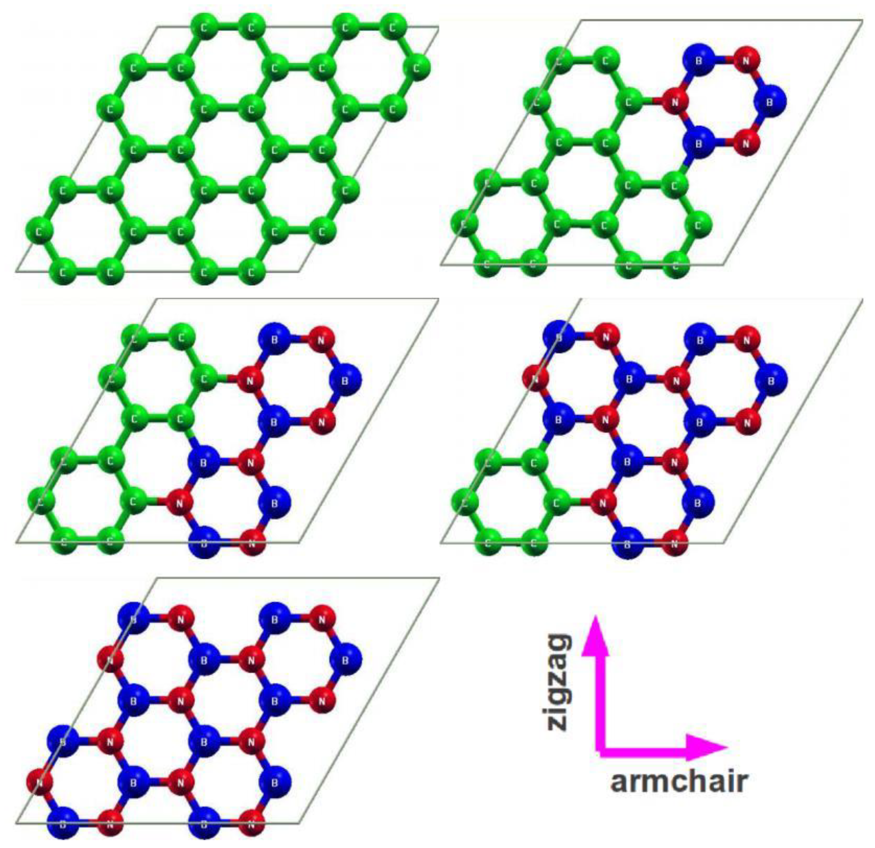
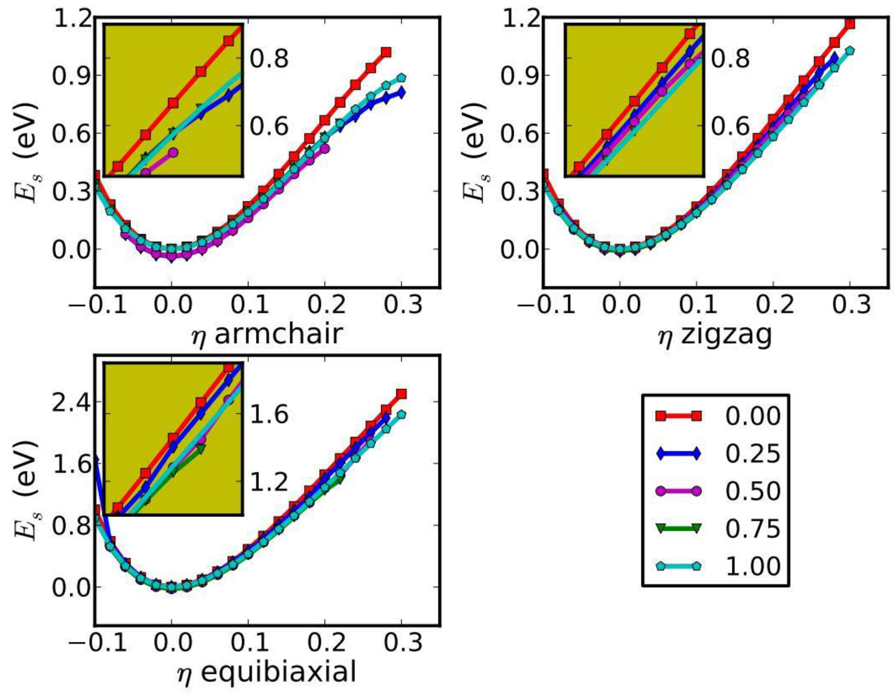
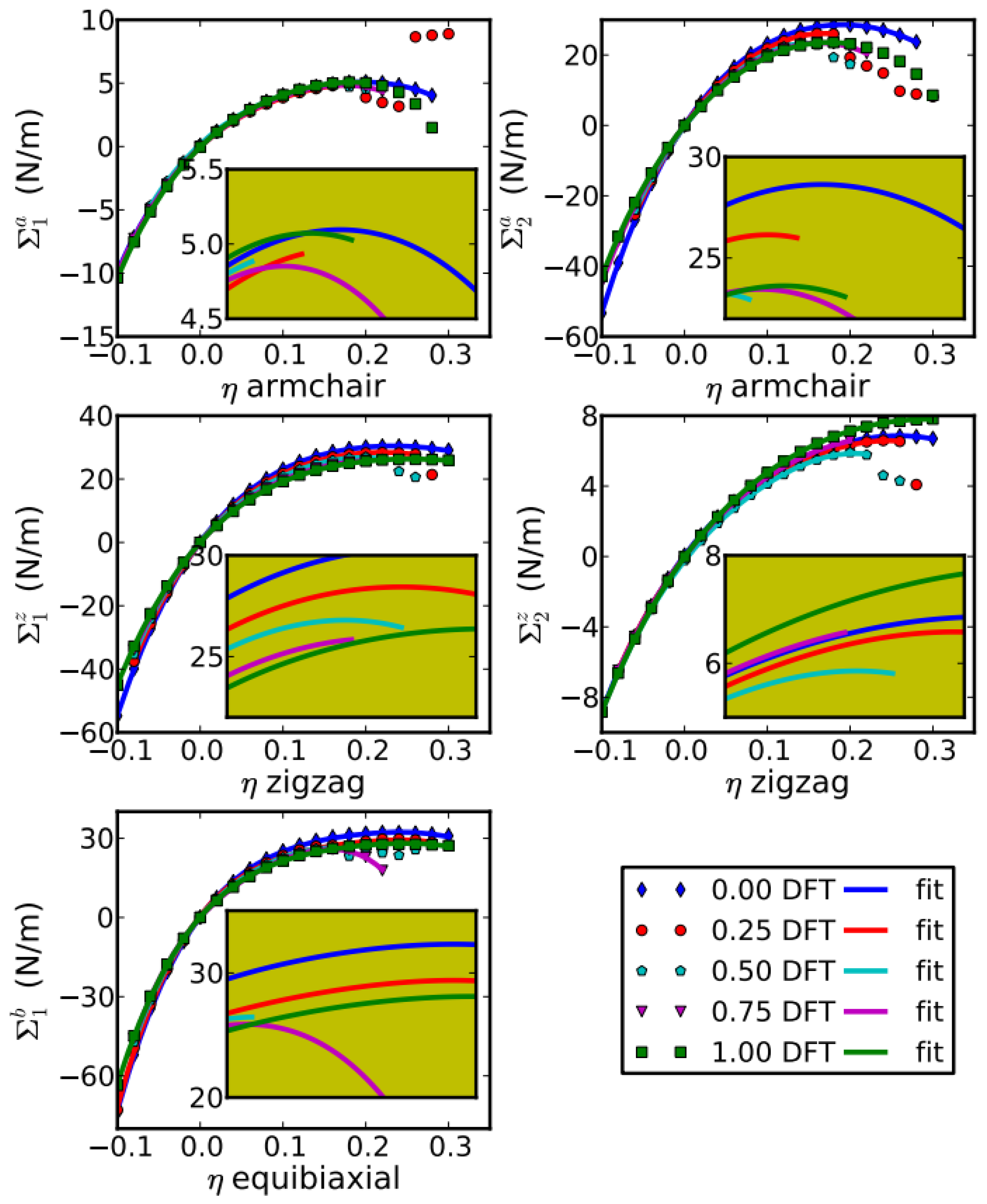
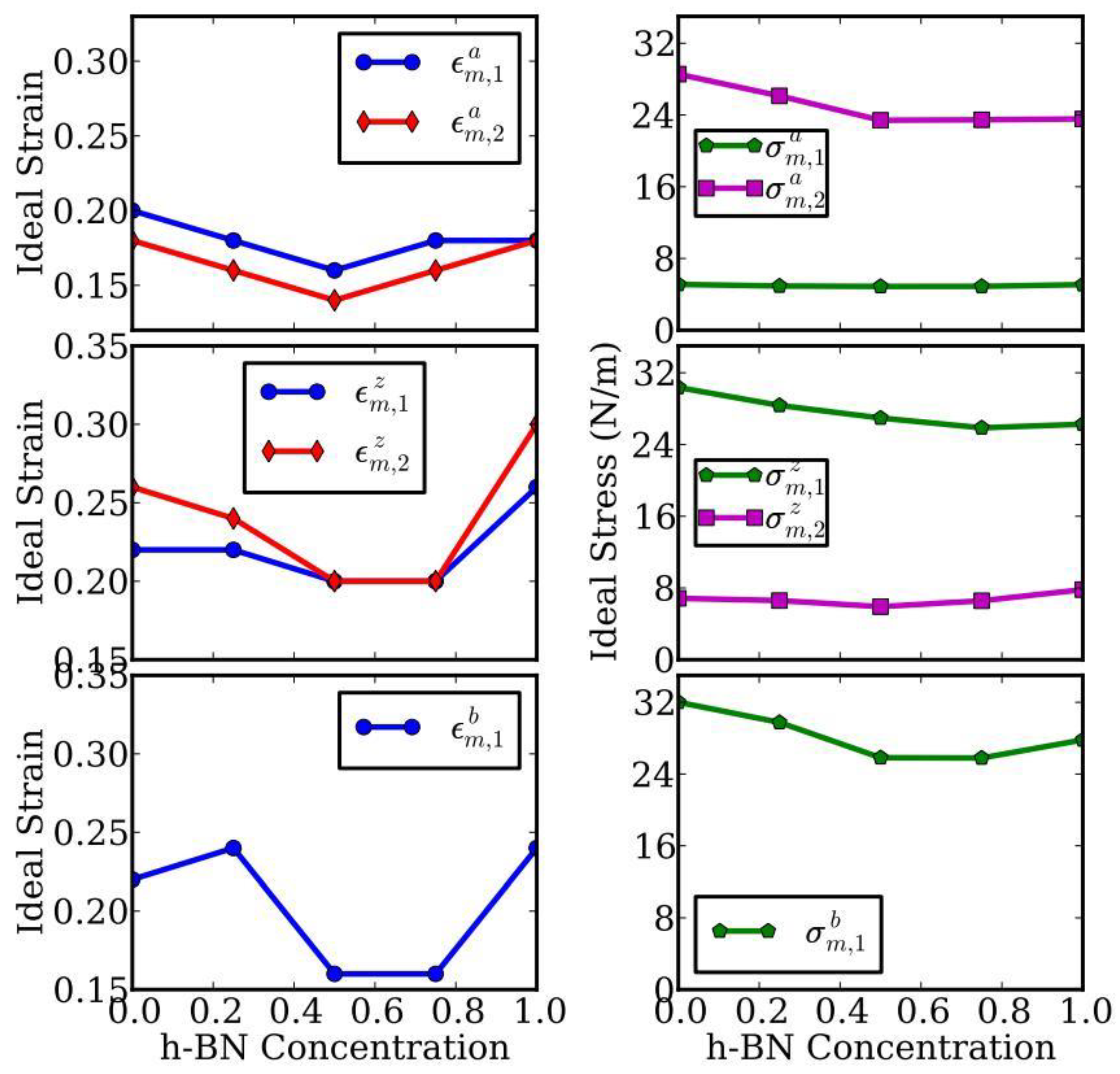
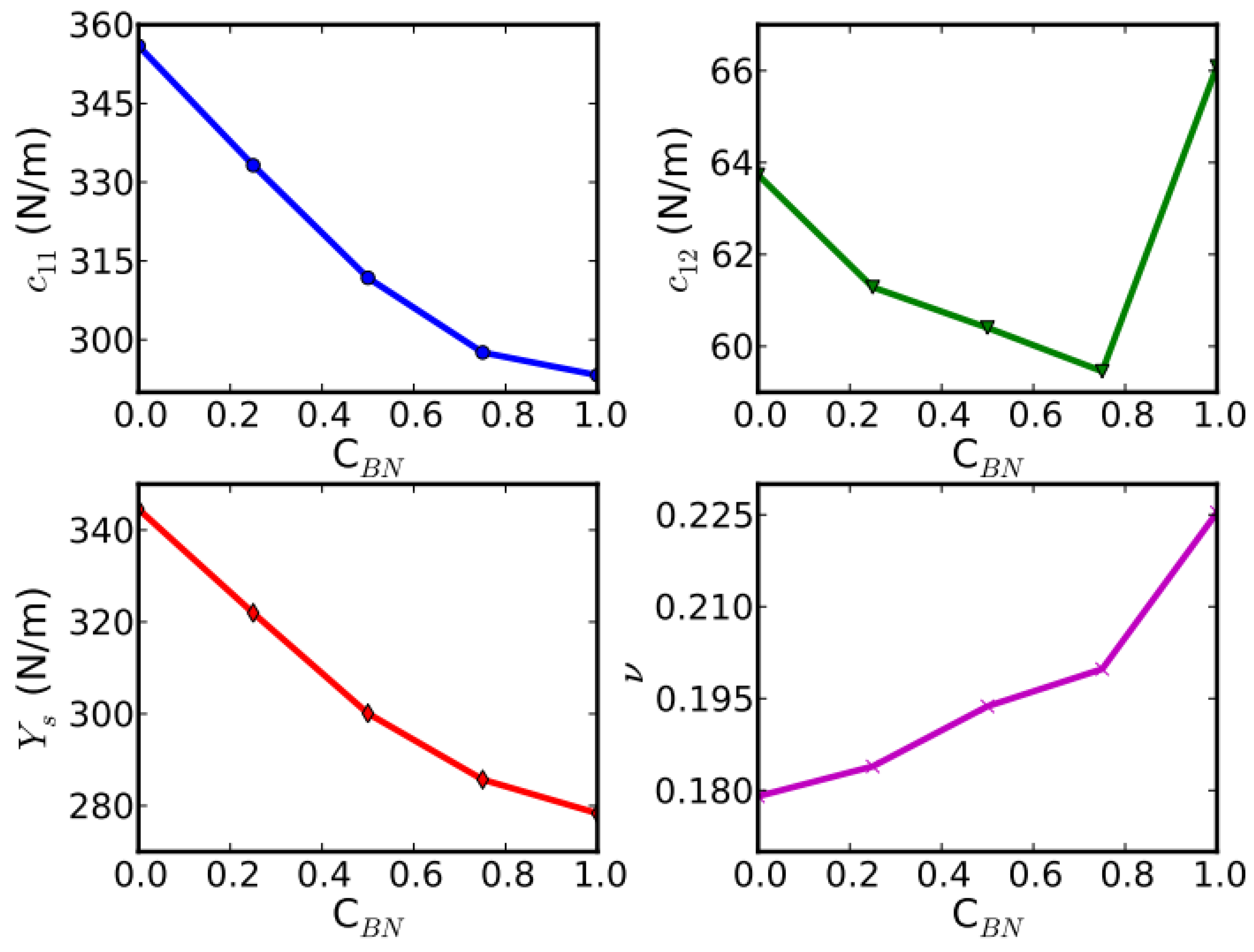
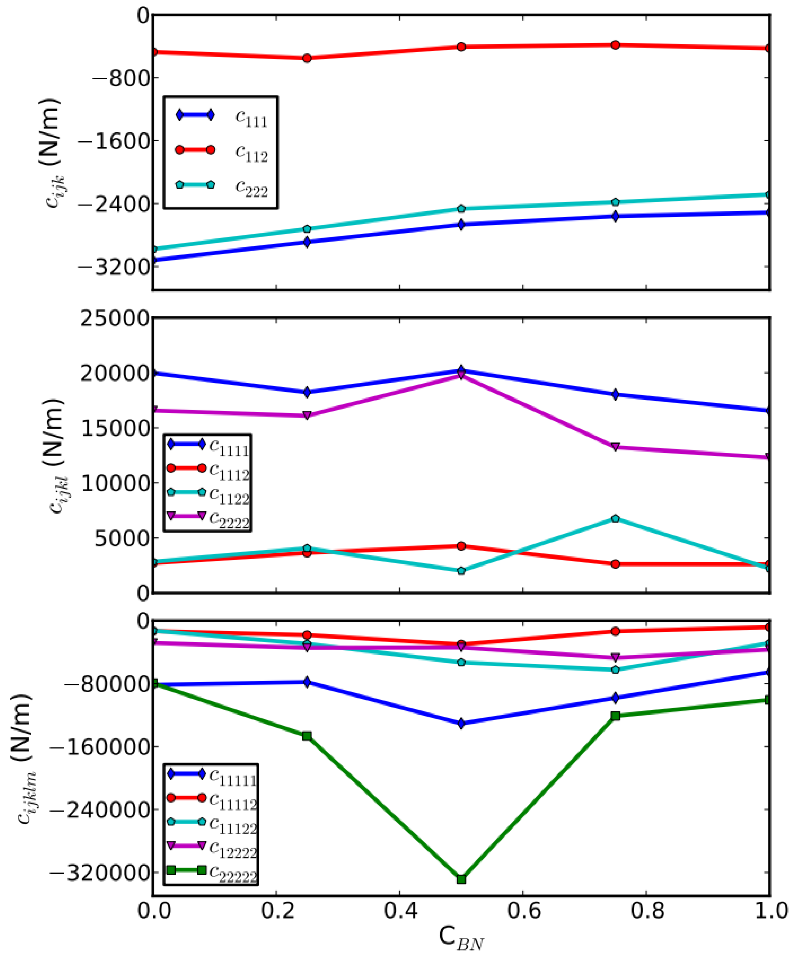
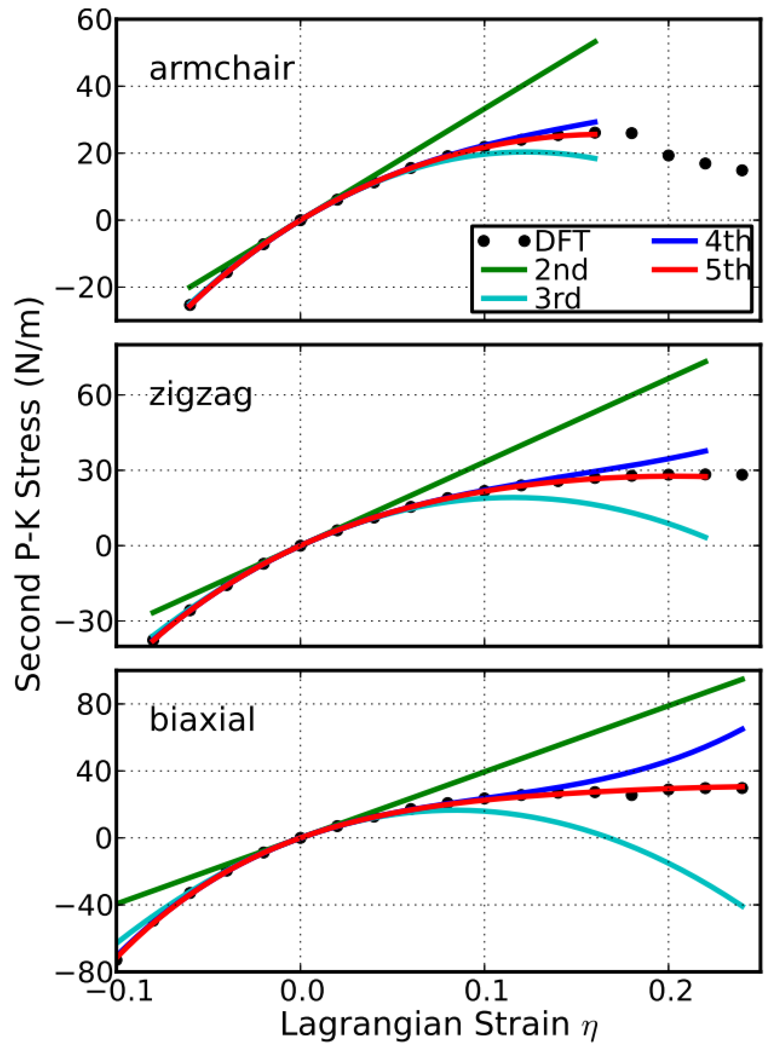
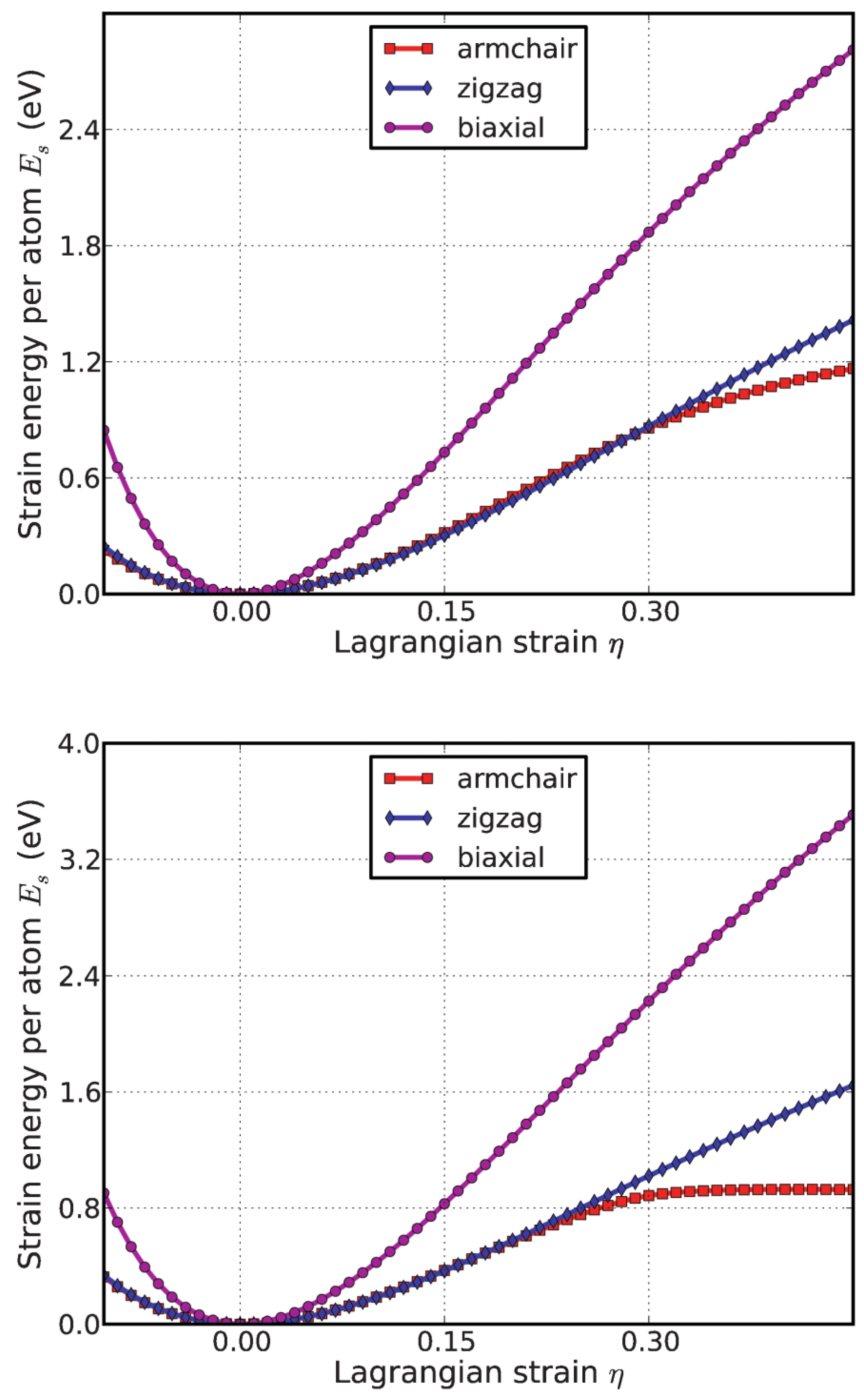
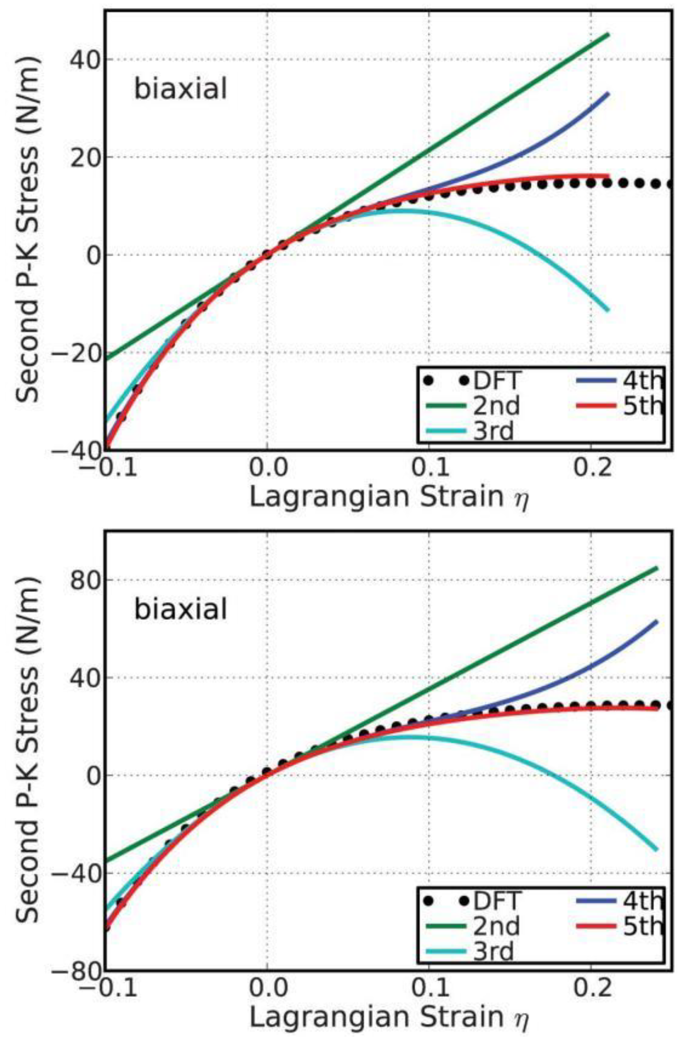
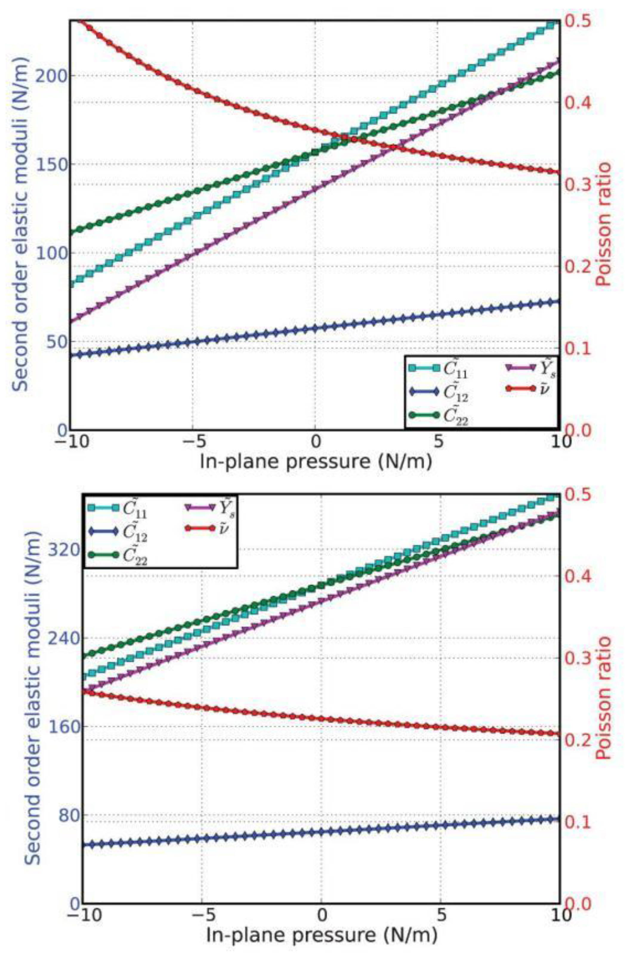
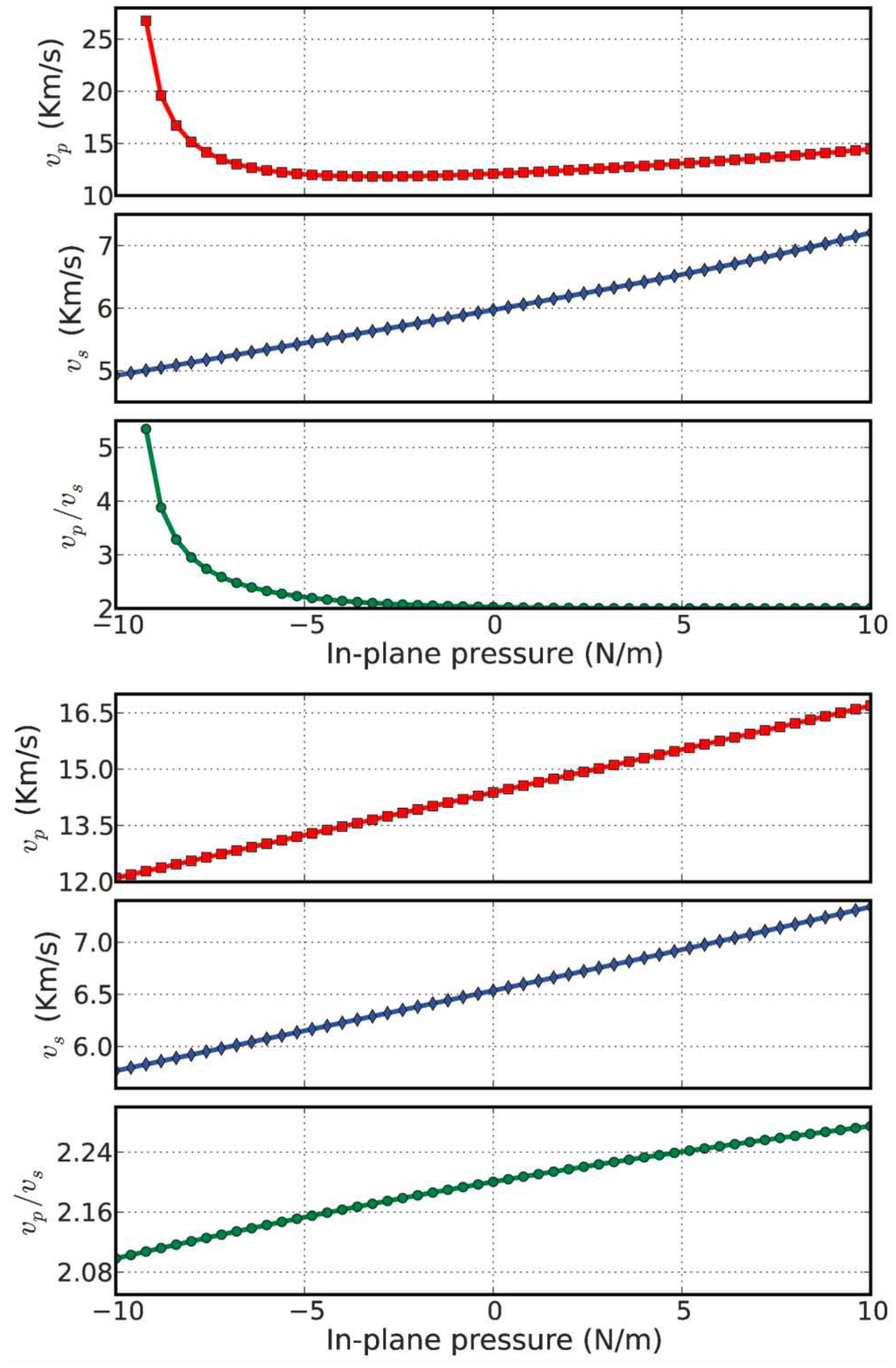
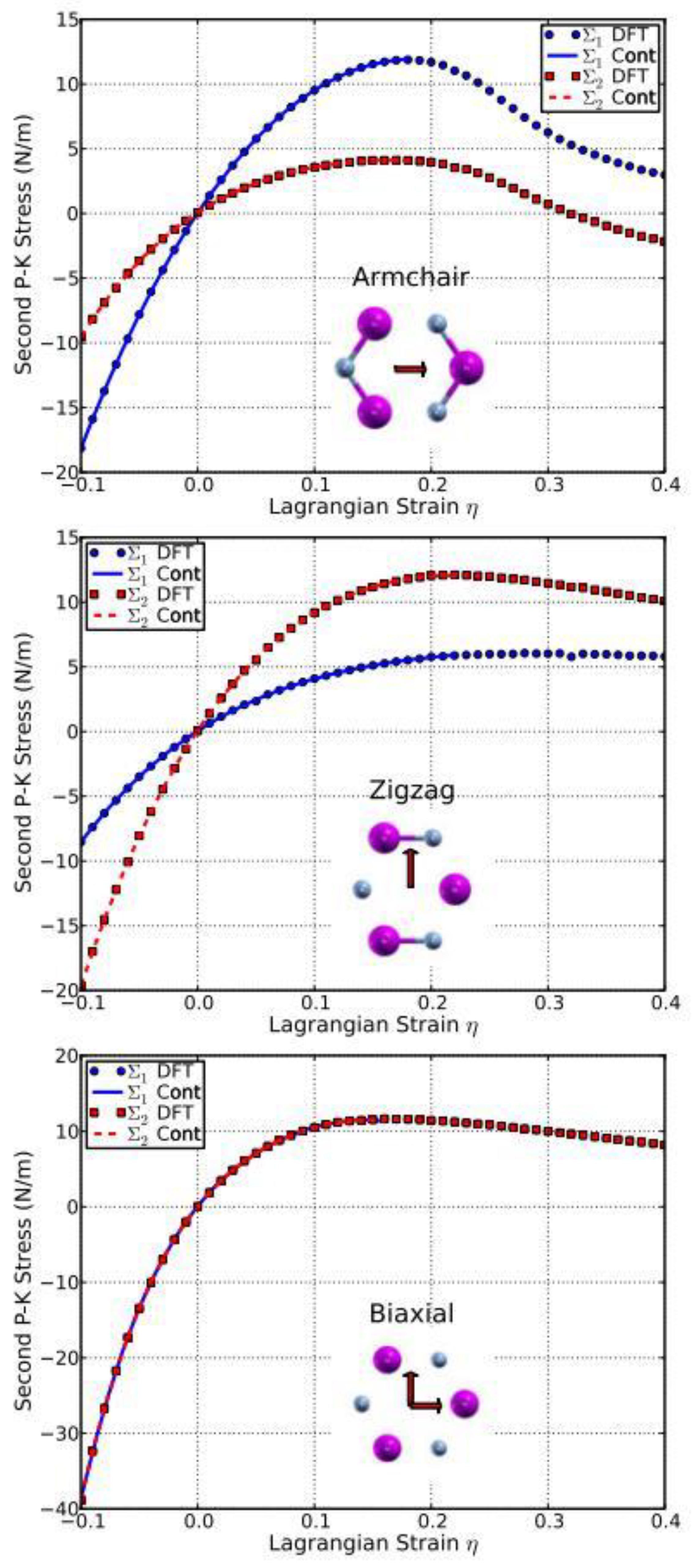
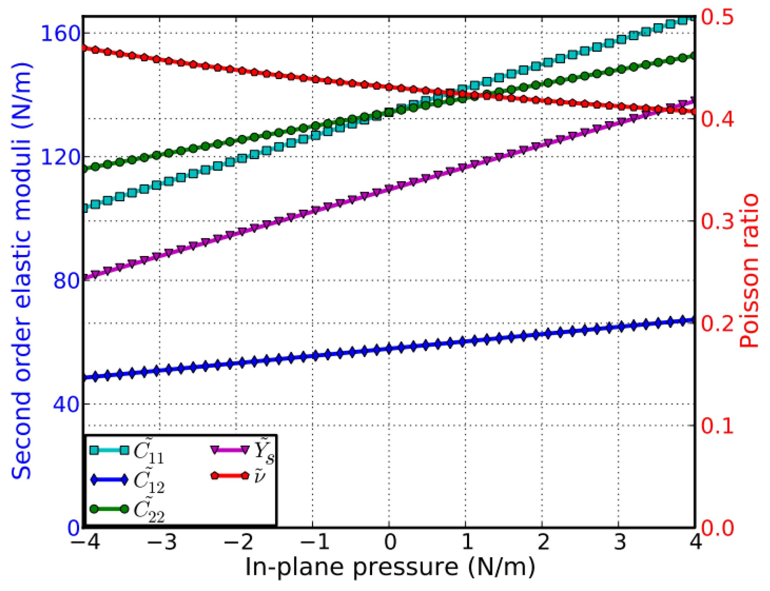
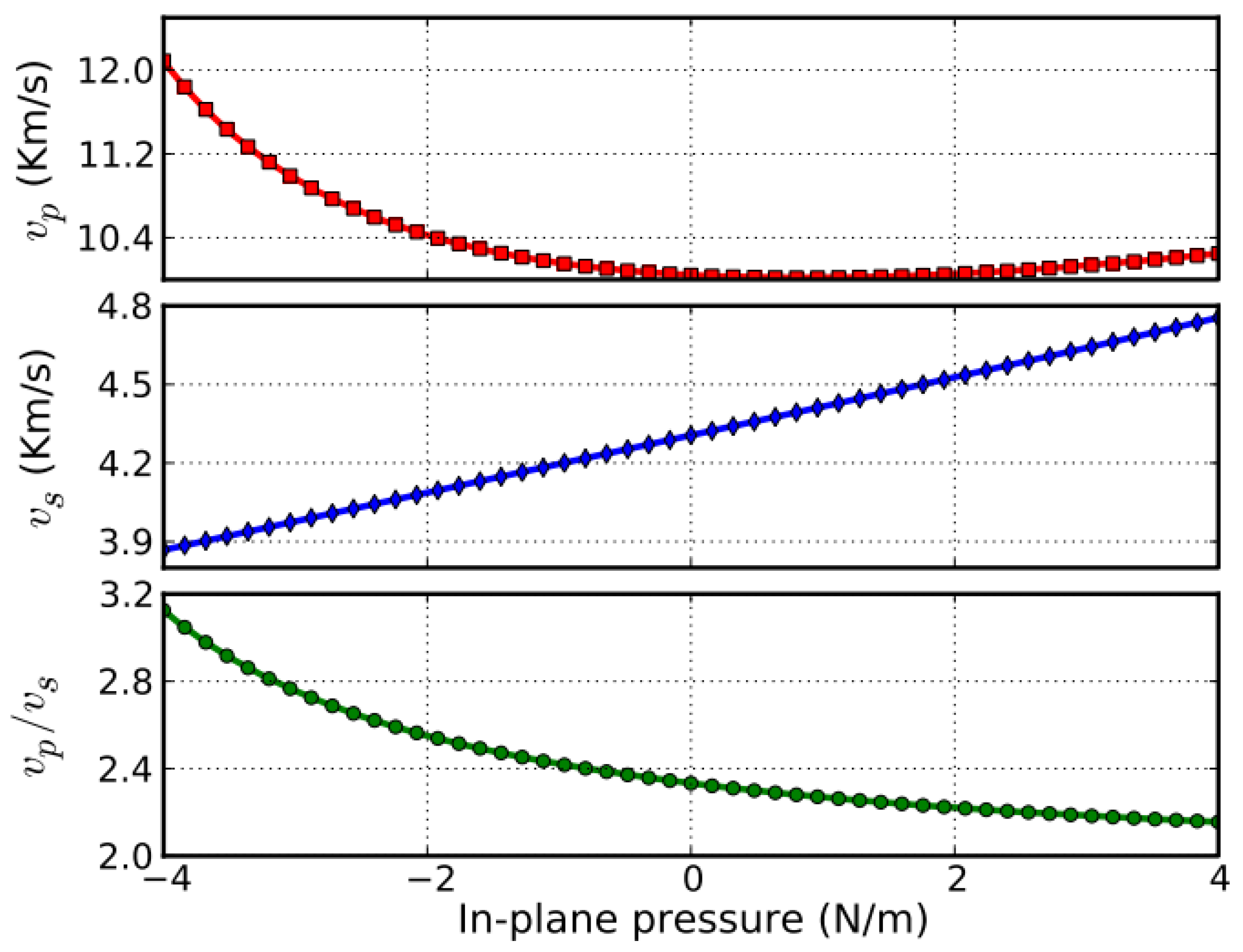
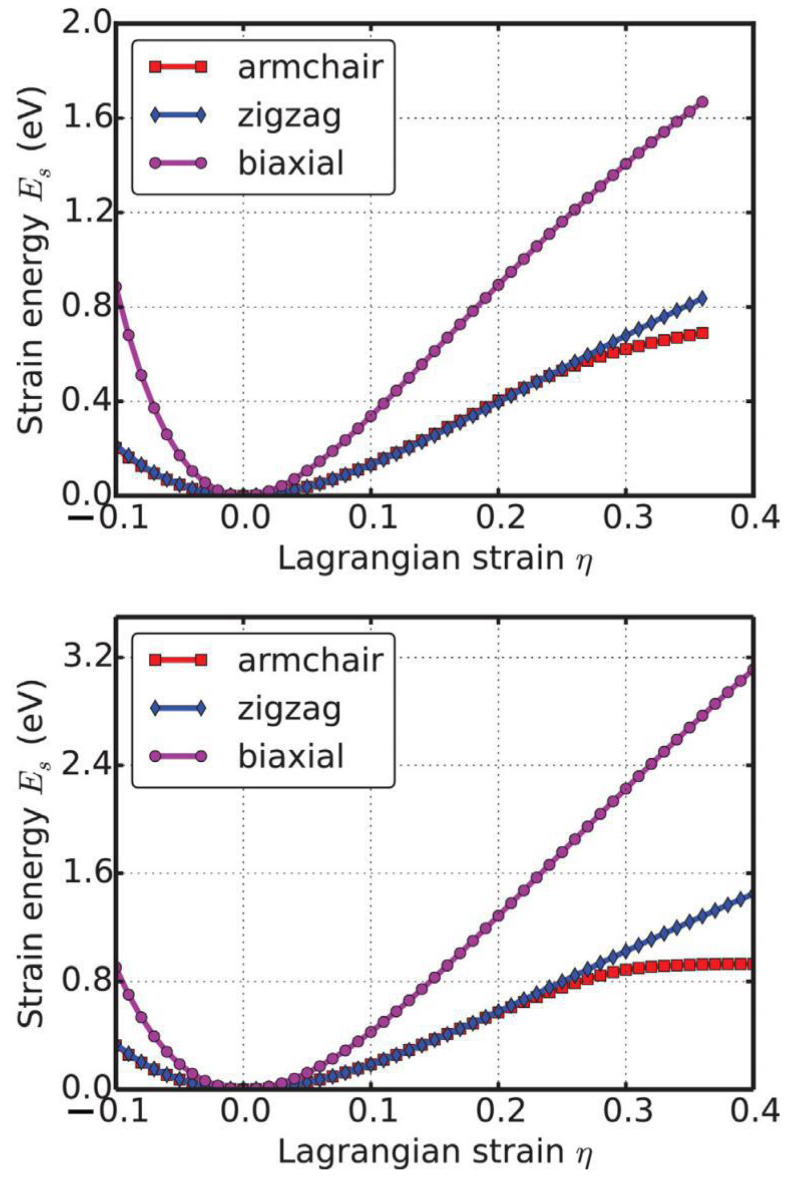
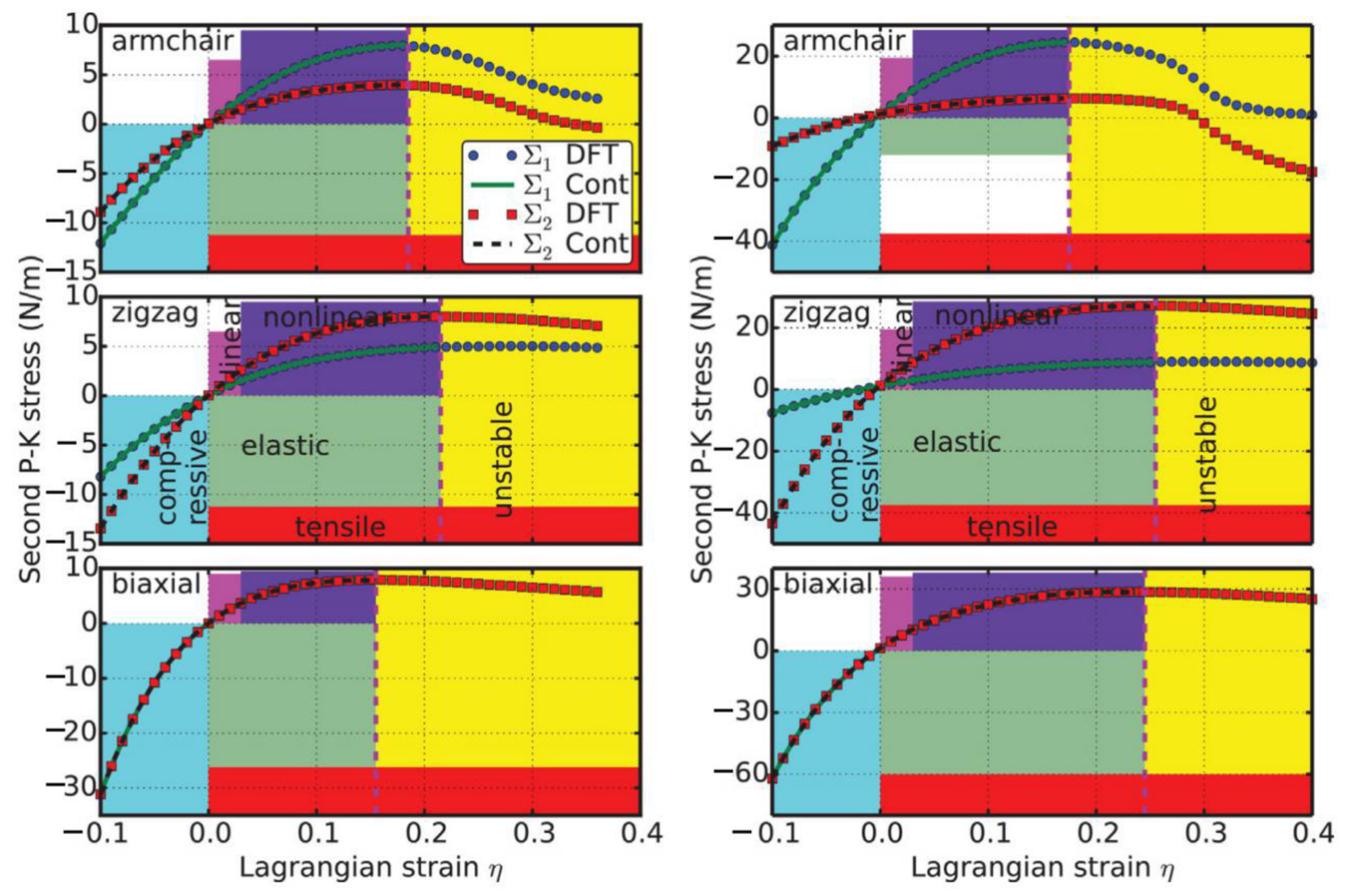
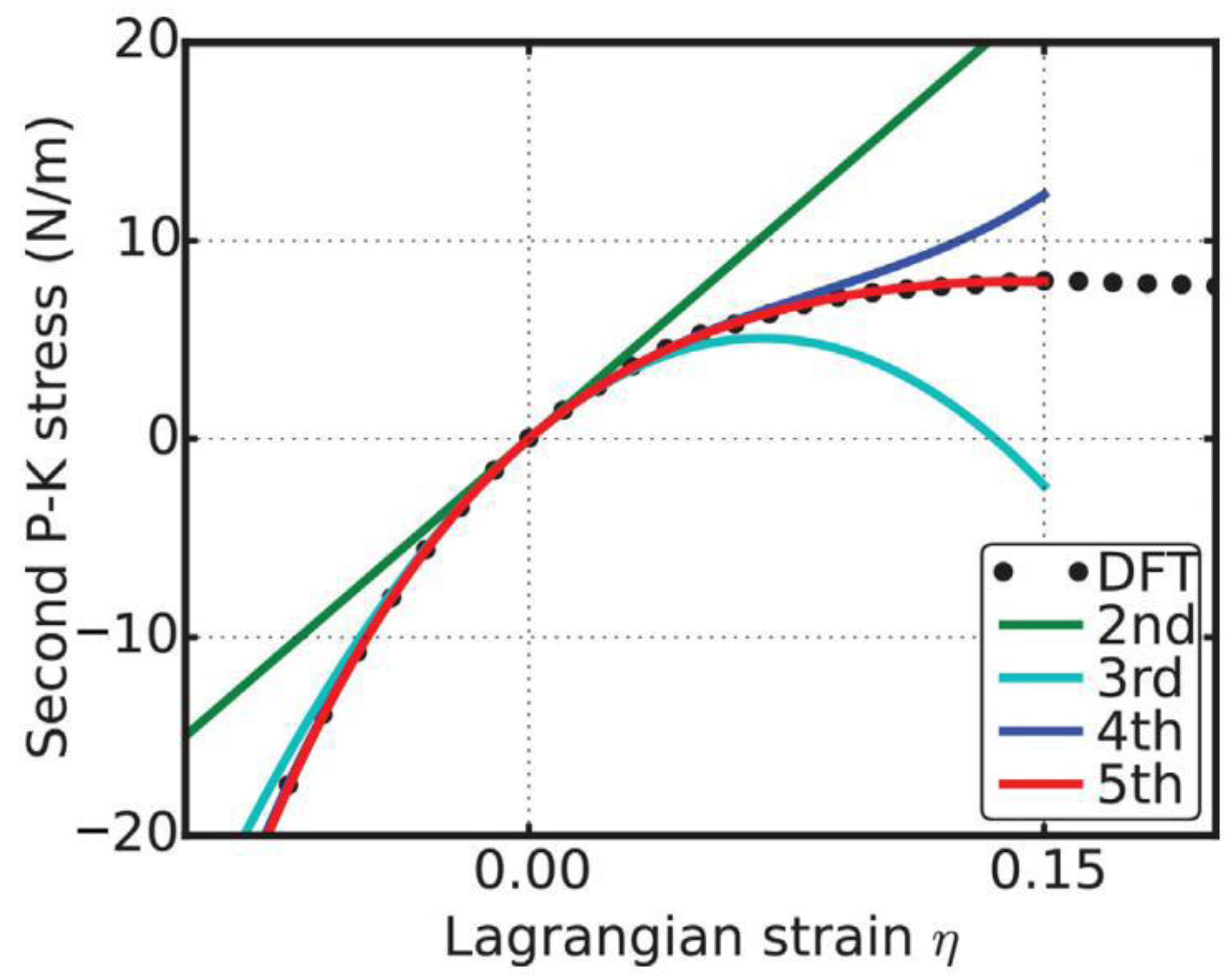
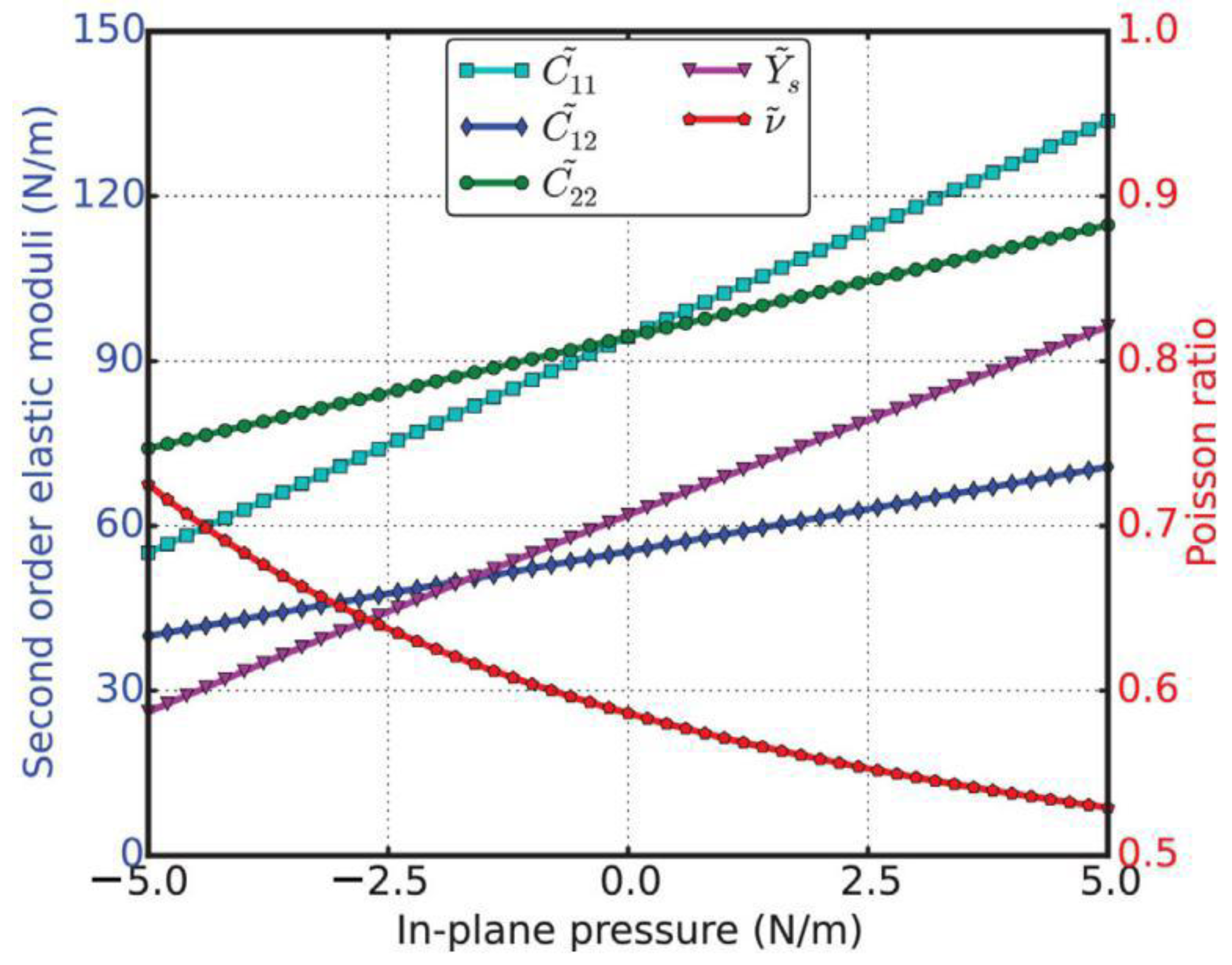
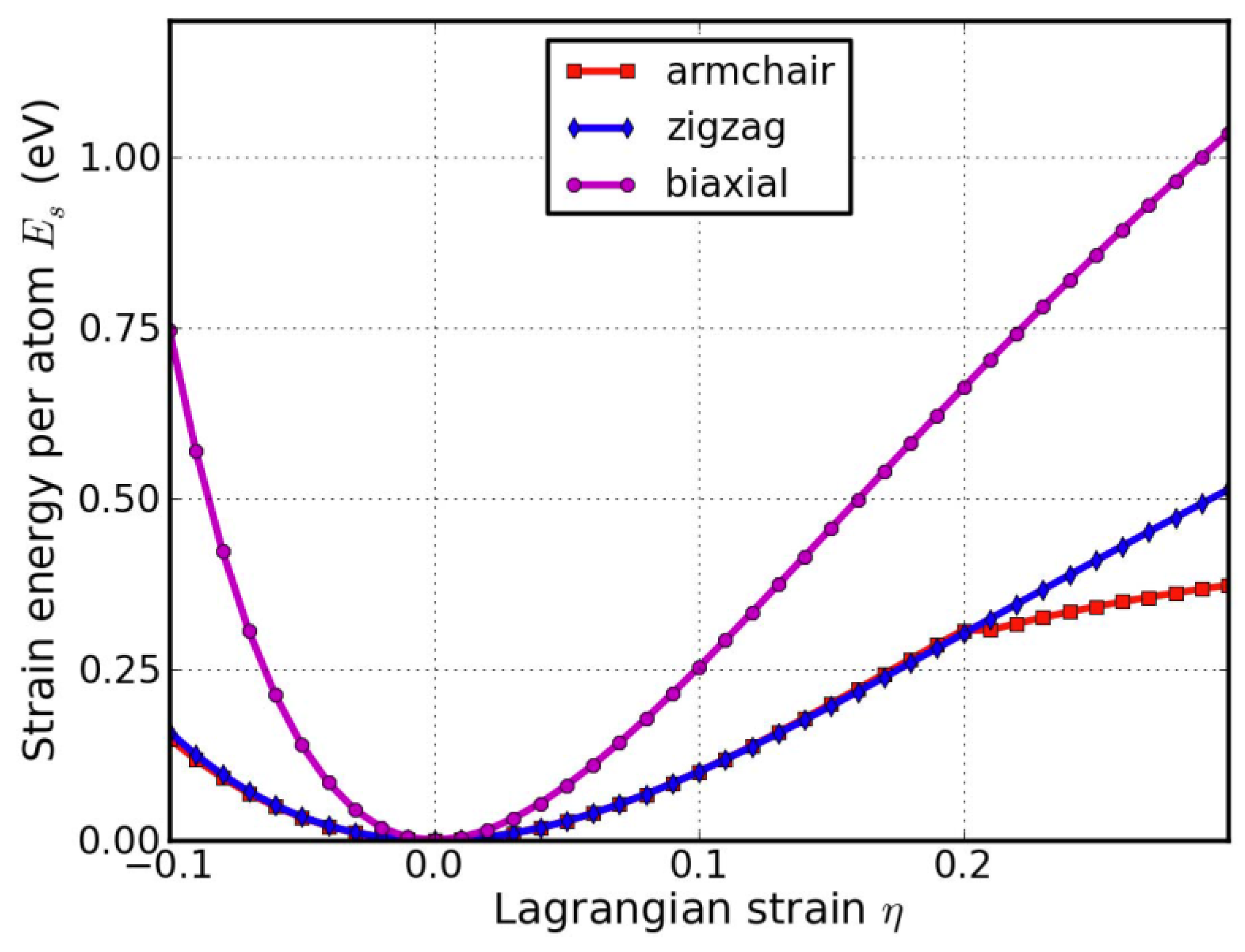
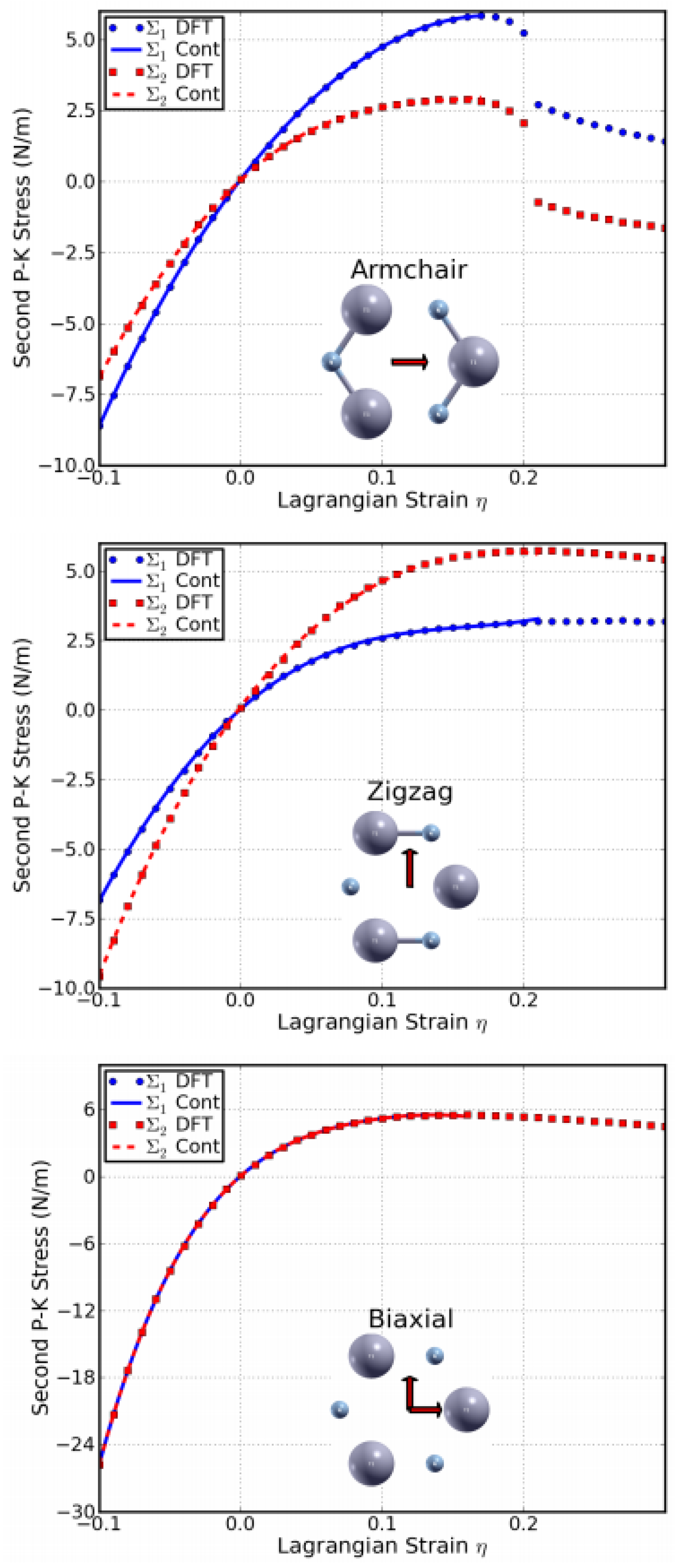
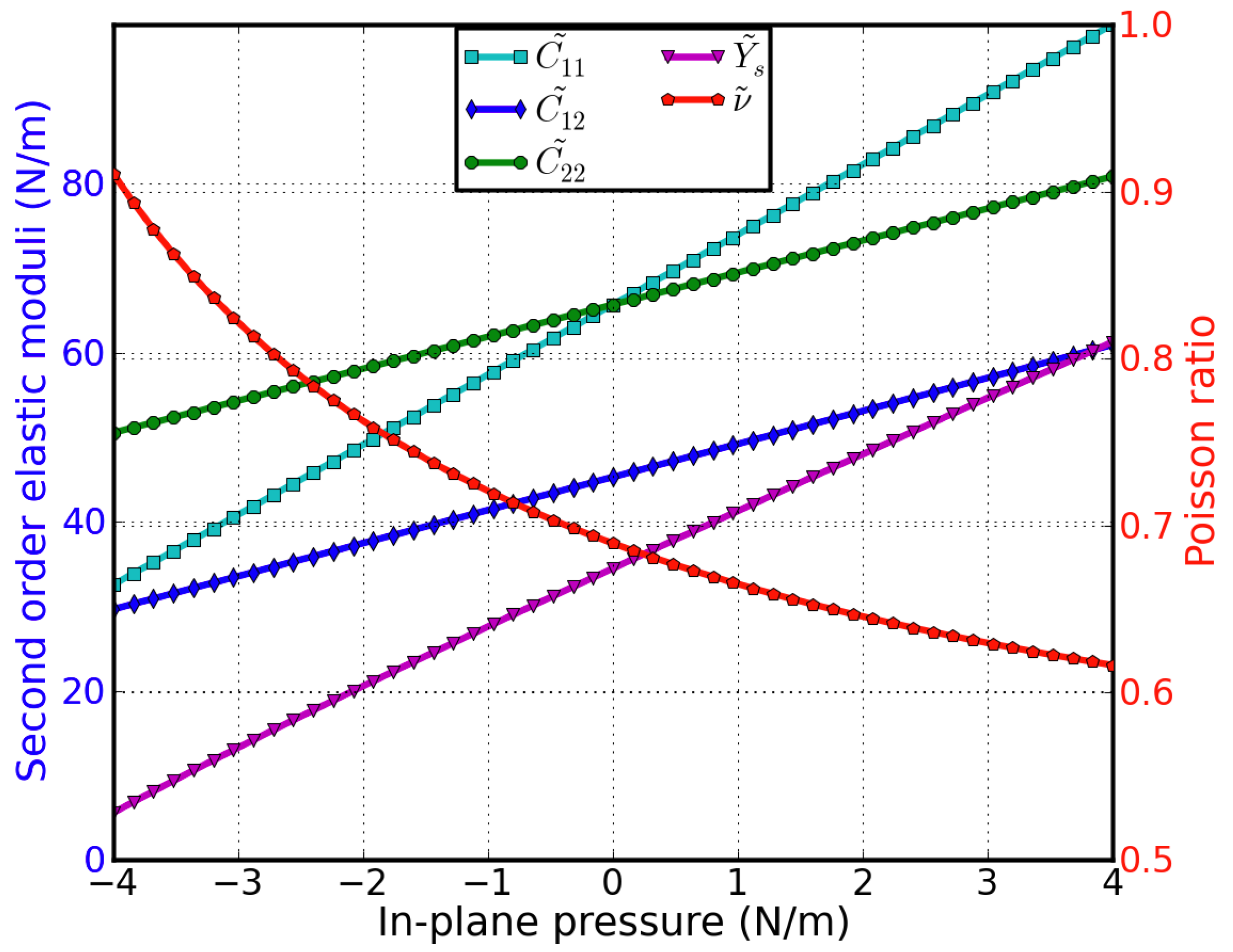
Table 1.
Lattice constants a, in-plane stiffness Ys, Poisson’s ratio ν, and high-order elastic constants of g-BNC from DFT calculations, compared to previous calculations of graphene.
Table 1.
Lattice constants a, in-plane stiffness Ys, Poisson’s ratio ν, and high-order elastic constants of g-BNC from DFT calculations, compared to previous calculations of graphene.
| 0.00 | 0.25 | 0.50 | 0.75 | 1.00 | Graphene a | |
|---|---|---|---|---|---|---|
| a | 2.468 | 2.484 | 2.496 | 2.506 | 2.512 | 2.446 |
| Ys | 344.6 | 321.9 | 300.0 | 285.7 | 278.3 | 348 |
| V | 0.1790 | 0.1839 | 0.1937 | 0.1998 | 0.2254 | 0.169 |
| Qi | 356.0 | 333.2 | 311.8 | 297.6 | 293.2 | 358.1 |
| C12 | 63.7 | 61.3 | 60.4 | 59.4 | 66.1 | 60.4 |
| Cm | −3121 | −2888 | −2666 | −2560 | −2514 | −2817 |
| C112 | −472 | −551 | −407 | −383 | −425 | −337 |
| C222 | −2978 | −2722 | −2466 | −2381 | −2284 | −2693 |
| Gm | 19,980 | 18,220 | 20,195 | 18,030 | 16,547 | 13,416 |
| C1112 | 2706 | 3643 | 4267 | 2628 | 2609 | 759 |
| C1122 | 2843 | 4065 | 2012 | 6755 | 2215 | 2582.8 |
| C2222 | 16,568 | 16,085 | 19,746 | 13,234 | 12,288 | 10,358.9 |
| Q11111 | −81,498 | −77,944 | −130,712 | −98,102 | −65,265 | −31,383.8 |
| Q11112 | −13,378 | −18,430 | −30,317 | −13,725 | −8454 | −88.4 |
| G11122 | −12,852 | −29,572 | −52,986 | −62,434 | −28,556 | −12,960.5 |
| G12222 | −28,504 | −34,777 | −34,287 | −47,317 | −36,955 | −13,046.6 |
| C22222 | −79,311 | −146,507 | −328,759 | −121,135 | −100,469 | −33,446.7 |
a Graphene in a 2-atom unit cell [46].
Table 2.
Ultimate strengths (Σma, Σmz, Σmb) in units of N m−1 and ultimate strains (ηma, ηmz, ηmb) under uniaxial strain (armchair and zigzag) and biaxial strain from DFT calculations, compared with g-BN, graphene, and graphyne.
Table 2.
Ultimate strengths (Σma, Σmz, Σmb) in units of N m−1 and ultimate strains (ηma, ηmz, ηmb) under uniaxial strain (armchair and zigzag) and biaxial strain from DFT calculations, compared with g-BN, graphene, and graphyne.
| g-BN | g-AlN | g-GaN | g-InN | g-TIN | |
|---|---|---|---|---|---|
| Σma | 23.6 | 16.2 | 11.9 | 8.0 | 5.8 |
| ηma | 0.18 | 0.22 | 0.18 | 0.18 | 0.17 |
| Σmz | 26.3 | 15.9 | 12.1 | 8.0 | 5.7 |
| ηmz | 0.26 | 0.27 | 0.22 | 0.21 | 0.21 |
| Σmb | 27.8 | 14.8 | 11.7 | 8.0 | 5.5 |
| ηmb | 0.24 | 0.21 | 0.16 | 0.15 | 0.16 |
Table 3.
Non-zero independent components for the SOEC, TOEC, FOEC, and FFOEC tensor components, Poisson’s ratio n, and in-plane stiffness Ys of g-AlN from DFT calculations, compared with g-BN, graphene, and graphyne.
Table 3.
Non-zero independent components for the SOEC, TOEC, FOEC, and FFOEC tensor components, Poisson’s ratio n, and in-plane stiffness Ys of g-AlN from DFT calculations, compared with g-BN, graphene, and graphyne.
| g-BN | g-AlN | g-GaN | g-InN | g-TlN | |
|---|---|---|---|---|---|
| A | 2.512 | 3.127 | 3.207 | 3.585 | 3.73 |
| Ys | 278.3 | 135.7 | 109.4 | 62.0 | 34.5 |
| Ν | 0.225 | 0.366 | 0.431 | 0.586 | 0.689 |
| C11 | 293.2 | 156.7 | 134.4 | 94.4 | 65.7 |
| C12 | 66.1 | 57.4 | 57.9 | 55.4 | 45.3 |
| C111 | −2513.6 | −1265.7 | −1038.6 | −716.7 | −485.2 |
| C112 | −425 | −328.3 | −452.2 | −461.0 | −434 |
| C222 | −2284.2 | −968.9 | −880.6 | −609.1 | −420.6 |
| C1111 | 16,547 | 8753 | 5478 | 2978 | 1977 |
| C1112 | 2609 | 699 | 2710 | 3307 | 623 |
| C1122 | 2215 | 4604 | 4964 | 2514 | 7317 |
| C2222 | 12,288 | 2447 | 2165 | −1745 | 1362 |
| C11111 | −65,265 | −46,941 | −22,786 | 3382 | −13,969 |
| C11112 | −8454 | −2801 | 12,073 | −591 | 16,509 |
| C11122 | −28,556 | −13,643 | −29,688 | −17,843 | −23,086 |
| C12222 | −36,955 | −18,237 | 26,909 | −9615 | 32,898 |
| C22222 | −100,469 | −3855 | −9539 | 40,801 | −11,812 |
Disclaimer/Publisher’s Note: The statements, opinions and data contained in all publications are solely those of the individual author(s) and contributor(s) and not of MDPI and/or the editor(s). MDPI and/or the editor(s) disclaim responsibility for any injury to people or property resulting from any ideas, methods, instructions or products referred to in the content. |
© 2022 by the authors. Licensee MDPI, Basel, Switzerland. This article is an open access article distributed under the terms and conditions of the Creative Commons Attribution (CC BY) license (https://creativecommons.org/licenses/by/4.0/).
Share and Cite
MDPI and ACS Style
Ye, C.; Peng, Q. Mechanical Stabilities and Properties of Graphene-like 2D III-Nitrides: A Review. Crystals 2023, 13, 12. https://doi.org/10.3390/cryst13010012
AMA Style
Ye C, Peng Q. Mechanical Stabilities and Properties of Graphene-like 2D III-Nitrides: A Review. Crystals. 2023; 13(1):12. https://doi.org/10.3390/cryst13010012
Chicago/Turabian StyleYe, Chao, and Qing Peng. 2023. "Mechanical Stabilities and Properties of Graphene-like 2D III-Nitrides: A Review" Crystals 13, no. 1: 12. https://doi.org/10.3390/cryst13010012
Note that from the first issue of 2016, this journal uses article numbers instead of page numbers. See further details here.