1. Introduction
A single quantum impurity is the simplest quantum many-body problem for which interaction plays a crucial role [
1,
2]. It was designed as a model to describe diluted magnetic impurities in a non-magnetic metallic host. In the 1960s, it was showed that the perturbation series in coupling strength diverges even with an infinitesimal anti-ferromagnetic coupling value [
1]. This early unexpected result motivated the development of innovative approaches to model the strongly correlated systems [
1,
2,
3].
While the physics of a single impurity problem has been rather well studied, interest in the quantum impurity problem was revived during the 1990s. This was partly due to the interest in mapping lattice models onto impurity models [
4,
5,
6,
7,
8], since at infinite dimensions, the lattice models are equivalent to single impurity models in a mean-field represented by the density of states of the host. This approximated mapping is known as the dynamical mean-field theory. It has been further generalized to cluster impurity models which include some of the effects present in finite dimensional systems [
9,
10,
11].
These mappings provide a systematic tractable approximation for the lattice models and have become a major approach in the field of strongly correlated systems [
11]. Combined with density functional theory, they provide one of the best available methods for the study of the properties of materials in which strong interactions are important [
12].
The mean-field where the single impurity is embedded, i.e., the density of the bath, can be rather complicated. Therefore, there is in general no analytic method for an accurate solution. Many different methods for solving the effective impurity problem have been proposed. They can be broadly divided in two categories: semi-analytic and numeric.
Between the semi-analytic methods, the most widely used one is the iterative perturbation theory. It interpolates the self-energy at both the weak and strong coupling limits and incorporates some exact constraints, such as the Luttinger theorem [
13]. Another widely used semi-analytic method is the local moment approximation. It considers the perturbation on top of the strong coupling limit represented by the unrestricted Hatree Fock solution [
14].
Numerical methods can also be divided into two main classes, diagonalization-based and Monte-Carlo-based. Diagonalization methods usually require discretizing the host by a finite number of so-called bath sites. The Hamiltonian which includes the bath sites and the impurity site are diagonalized exactly [
15]. Another digonalization-based method is the numerical renormalization group in which the bath sites are mapped onto a one-dimensional chain of sites. The hopping amplitude decreases rapidly down the chain. The model is then diagonalized iteratively as more sites are included [
16]. Density matrix renormalization group and coupled cluster theory have also been used as impurity solvers [
17,
18,
19,
20].
Hirsh and Fye were the first to propose the quantum Monte Carlo method for solving impurity problems [
21]. The time axis of the simulations is divided up using the Trotter–Suzuki approximation. The interaction in each time segment is handled by the Hubbard–Stratonovich approximation [
22]. The Monte Carlo method is then used to sample the Hubbard–Stratonovich fields. Continuous time quantum Monte Carlo methods have seen a lot of development over the last decade. They directly sample the partition function without using the Trotter–Suzuki approximation [
23], similar to the Stochastic Series Expansion in the simulation of quantum spin models. Notably, the continuous time quantum Monte Carlo using the expansion with respect to the strong coupling limit has been proposed and complicated coupling functions beyond simple Hubbard local density-density coupling terms can now be studied [
24].
On the other hand, the past few years have seen tremendous development of machine learning (ML), both algorithms and their implementation [
25,
26,
27]. Many of the ML approaches in physics are designed to detect phase transitions or accelerate Monte Carlo simulations. It is a tantalizing proposal to utilize ML approaches to build a solver for quantum systems.
To build a quantum solver based on the ML approach, we need to identify the feature vector (input data) and the label (output data) for the problem. Then a large pool of data must be generated to train the model, specifically a neural network model. The Anderson impurity problem is a good test bed for the validity of such a solver. We note that similar ideas have been explored using machine learning approaches [
28]. This paper is focused on using the kernel polynomial expansion and supervised ML, specifically a neural network, as the building blocks for a quantum impurity solver.
While it is relatively inexpensive to solve a single impurity problem using the above methods in modern computing facilities, current interest in the effects of disorder warrants the new requirement of solving a large set of single or few impurities problems in order to calculate the random disorder average [
29,
30,
31,
32,
33,
34,
35]. Our hope is that a fast neural-network-based numerical solver in real frequency can expand the range of applicability of the recently developed typical medium theory to interacting strongly correlated systems, such as the Anderson–Hubbard model [
36,
37,
38,
39].
This paper is organized as follows. In the next section, we map the continuous Green function into a finite cluster as has been performed in many dynamical mean field theory calculations. In
Section 3, we discuss the expansion of the spectral function in terms of Chebyshev polynomials. In
Section 4, we discuss how to use the results from
Section 2 and
Section 3 as the feature vectors and labels of the neural network. In
Section 5, we present the spectral function calculated by the neural network approach. We conclude and discuss future work in the last section.
2. Representing the Host by a Finite Number of Bath Sites
We first identify the input and the output data of a single impurity Anderson model. The input data includes the bare density of states, the chemical potential and the Hubbard interaction on the impurity site. For a system in the thermodynamic limit, the density of states is represented by a continuous function. Since inputting a continuous function to the neural network presents a problem, we describe the continuous bath by a finite number of poles as it is performed within the exact diagonalization approach [
15,
40,
41,
42,
43]. We approximate the host Green function by a cluster of bath sites,
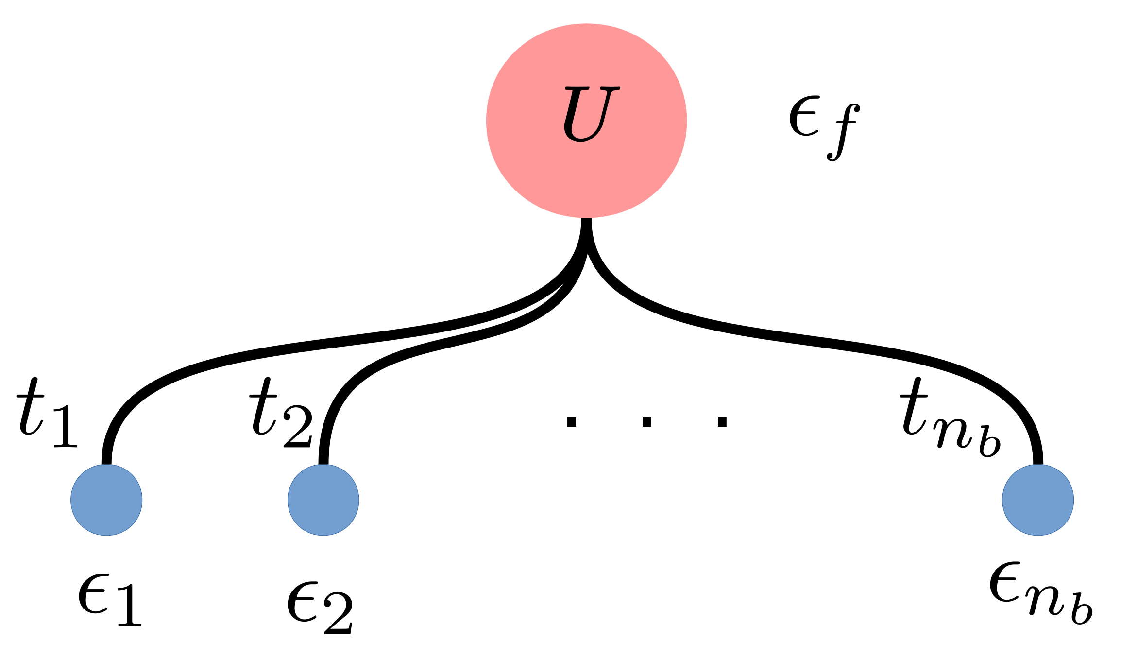
In the exact diagonalization method, the continuum bath is discretized and represented by a finite number of so-called bath sites, see
Figure 1. Assuming that there are
bath sites, each bath site is characterized by a local energy (
) and a hopping (
) term to the impurity site. Two additional variables, one the local Hubbard interaction (
U) and the other the chemical potential (
), are required to describe the impurity site. Therefore, there is a total of
variables representing the impurity problem.
The full Hamiltonian in the discretized form (
Figure 1) is given as
and are the creation and annihilation operators for site i with spin , respectively. The impurity site is denoted as the 0-th site. The sum of the bath sites goes from 1 to , and the spin .
The host Green function represented in such a finite cluster can be written exactly as,
Many different prescriptions for the parameterization of the host Green function have been investigated in detail for exact diagonalization solvers [
44]. Conceptually, practical applications of the numerical renormalization group method also require the approximated mapping of the problem onto a finite cluster chain. Unlike the exact diagonalization method, the cluster chain can be rather large; therefore much higher accuracy can be attained in general.
These approaches do not mimic the continuum in the time dimension as it is done by continuous time Quantum Monte Carlo methods, and the mapping onto the finite cluster may represent a nuisance. Nonetheless, this is a necessity for any diagonalization-based method. In our case, the mapping presents an opportunity to naturally adapt the method to a machine learning approach in which a finite discretized set of variables is required.
Under the above approximation, the finite set of variables,
, can be treated as the input feature vector for the machine learning algorithm. The next question is what is the desired output or label. We will focus on the spectral function in this study. For this purpose, the next step is to represent the spectral function with a finite number of variables instead of a continuous function. The kernel polynomial method fulfills this goal [
45].
3. Expanding the Impurity Green Function by Chebyshev Polynomials
In this section, we briefly discuss the kernel polynomial method for the calculation of the spectral function of a quantum interacting model. Once the host parameters, the impurity interaction and chemical potential are fixed, the ground state of the cluster is obtained using a diagonalization method for sparse matrices. We use the Lanczos approach in the present study [
46,
47]. Once the ground state is found, the spectral function can be calculated by applying the resolvent operator,
, to the ground state. A popular method is the continuous fraction expansion [
47]. The challenge is that the continuous fraction tends to be under-damped and produce spurious peaks [
46,
47]. A more recent method is to use an orthogonal polynomial expansion. We will argue that for the application of the ML method, the polynomial expansion method tends to produce better results as we will explain later [
45].
The zero temperature single particle retarded Green function corresponding to a generic many-body Hamiltonian is defined as
where
is the ground state of
H, and
and
c are the creation and annihilation operators, respectively [
45,
48]. The spectral function is given as
.
Consider the Chebyshev polynomials of the first kind defined as
. Two important properties of the Chebyshev polynomial are their orthogonality and their recurrence relation. The product of two Chebyshev polynomials integrated over
and weighted by the function
is given as
The recurrence relation is given as
The Chebyshev polynomials expansion method is based on the fact that the set of Chebyshev polynomials form an orthonormal basis as defined in Equation (
5). Thus a function,
, defined within the range of
can be expanded as
and the expansion coefficient can be obtained by the inner product of the function
and the Chebyshev polynomials as follow
Practical calculations involve truncation at a finite order. The truncation is found to be problematic when the function to expand is not smooth. In our problem, the function is the spectral function of a finite size cluster, which is a linear combination of a set of delta functions. For this reason, a direct application of the above formula will not provide a smooth function. This is analogue to the Gibbs oscillations in the Fourier expansion. The remedy is to introduce a damping factor (kernel) in each coefficient of the expansion [
45,
49,
50,
51,
52]. Here we use the Jackson kernel given as
We refer the choice of the damping factor to the review by Weiße et al. [
45].
We list the steps for calculating the coefficients as follows.
The input bare Green function is approximated by the bare Green function of a finite size cluster. The set of parameters
are obtained by minimizing the difference between the left-hand side and the right-hand side of Equation (
1) according to some prescriptions [
15,
40,
41,
42,
43].
The ground state and the corresponding energy are obtained by the Lanczos algorithm.
The spectrum of the Hamiltonian is scaled within the range [−1,1] as required by the Chebyshev expansion. , where a is a real positive constant. The units of energy are also scaled in terms of a.
The expansion coefficients are given by the inner product between the spectral function and the Chebyshev polynomials.
where
and
. With the
and the
ready, all the higher order coefficients can be obtained via the recurrence relation
The spectral function is obtained by feeding the coefficients into Equation (
7).
All the coefficients can be obtained by repeated use of Equation (
12) which involves matrix vector multiplication. The matrix for an interacting system is usually very sparse, and the computational complexity of the matrix vector multiplication is linear with respect to the vector length, which grows as
assuming no reduction by symmetry is applied.
Since practical calculations are limited to a finite order,
N, the impurity Green function can be represented by
N coefficients of the Chebyshev polynomials expansion. It is worthwhile to mention that the expansion of the Green function in terms of orthogonal polynomials is independent of the method for obtaining the coefficients of the polynomials. Instead of employing exact diagonalization, a recent study shows that one can obtain the expansion coefficients by representing the quantum states by matrix products [
48].
4. Feature Vectors and the Labels for the Machine Learning Algorithm
Our strategy is to train a neural network with a large set of variables for the host, i.e., the bath sites, the impurity interaction and the impurity chemical potential. The impurity solver calculates the impurity Green function for a given bath Green function, local impurity interaction and chemical potential that is a total of variables for the input.
The output is the impurity Green function which can be represented by N coefficients of the Chebyshev polynomials expansion. Using the above method, the spectral function is effectively represented in terms of N coefficients. It allows us to naturally employ the supervised learning method by identifying the variables as the input feature vectors and the N variables as the output labels.
While the kernel polynomial method grows exponentially with the number of sites, the end result is represented by a finite number of coefficients which presumably does not scale exponentially with the number of sites. Once the neural network is properly trained, we can use it to predict the impurity Green function without involving a calculation which scales exponentially.
5. Results
We generated 5000 samples for training the neural networks with randomly chosen parameters which are drawn uniformly from the range listed as follows:
We assume that the electron bath has a symmetric density of states. That is, and for to and even. This further reduces the number of variables in the feature vector to .
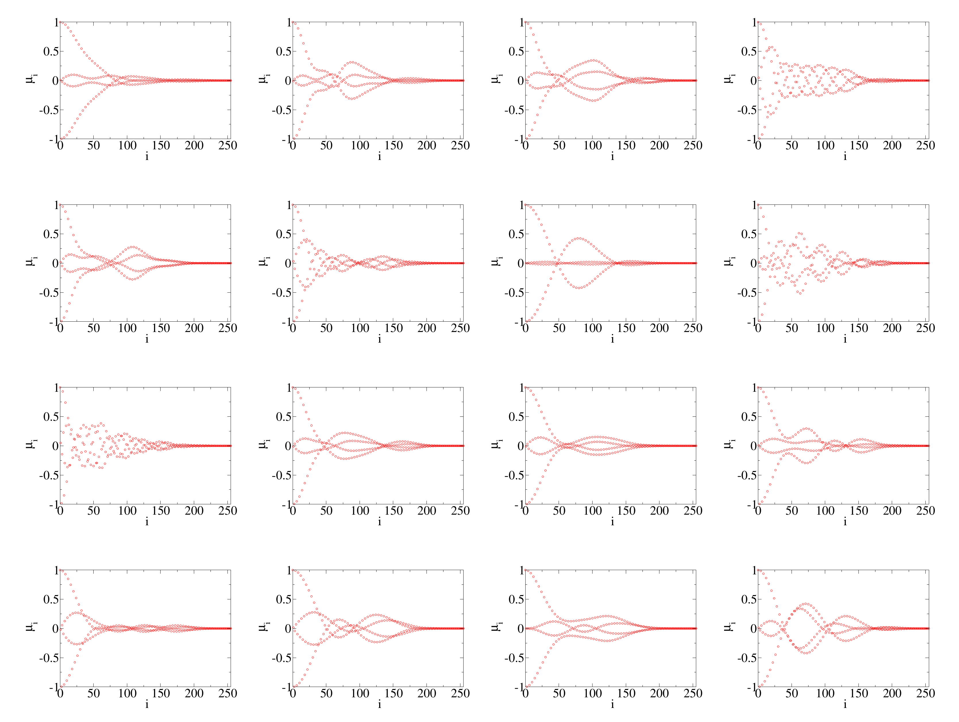
Before embarking on training the neural network, we would like to have some understanding of the range of Chebyshev coefficients. For this purpose, we randomly pick 32 samples and plot the coefficients in
Figure 2. There are two prominent features of the coefficients: 1. There are clear oscillations and the coefficients do not decrease monotonically. 2. For all cases shown here, the coefficients essentially vanish for orders around 200 and higher. Due to these two reasons, we decide to train the neural network for the coefficients between 0 and 255.
With the above approximations, the task of solving the Anderson impurity model boils down to mapping a vector containing variables to a vector containing N coefficients. For the particular case, we study we choose and . Machine learning algorithms can thus be naturally applied to this mapping.
We set up an independent dense neural network for each coefficient. The neural network has 14 layers. The input layer contains units, and the output layer contains the expansion coefficient for one specific order. The 12 hidden layers have the following number of units: .
As we consider a total of 256 orders, we train 256 independent neural networks. Considering the coefficients at different orders separately may lose some information contained in the correlations between them. While it is possible to predict a few coefficients by only one neural network, we do not obtain a good prediction using a single neural network for all 256 coefficients without an elaborated fine tuning. Therefore, here instead of searching for a optimal number of coefficients to be predicted for one neural network, we consider each coefficient independently.
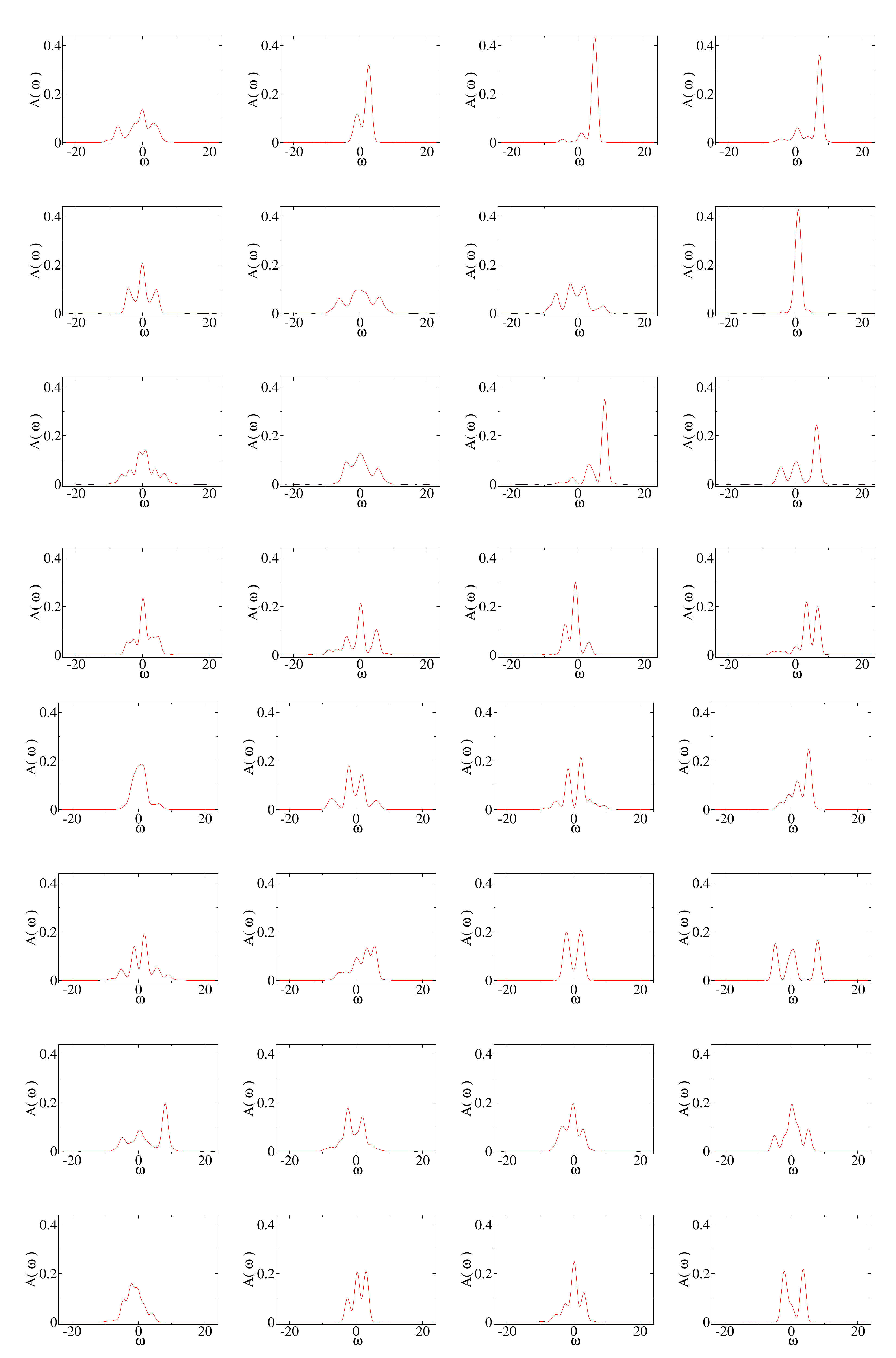
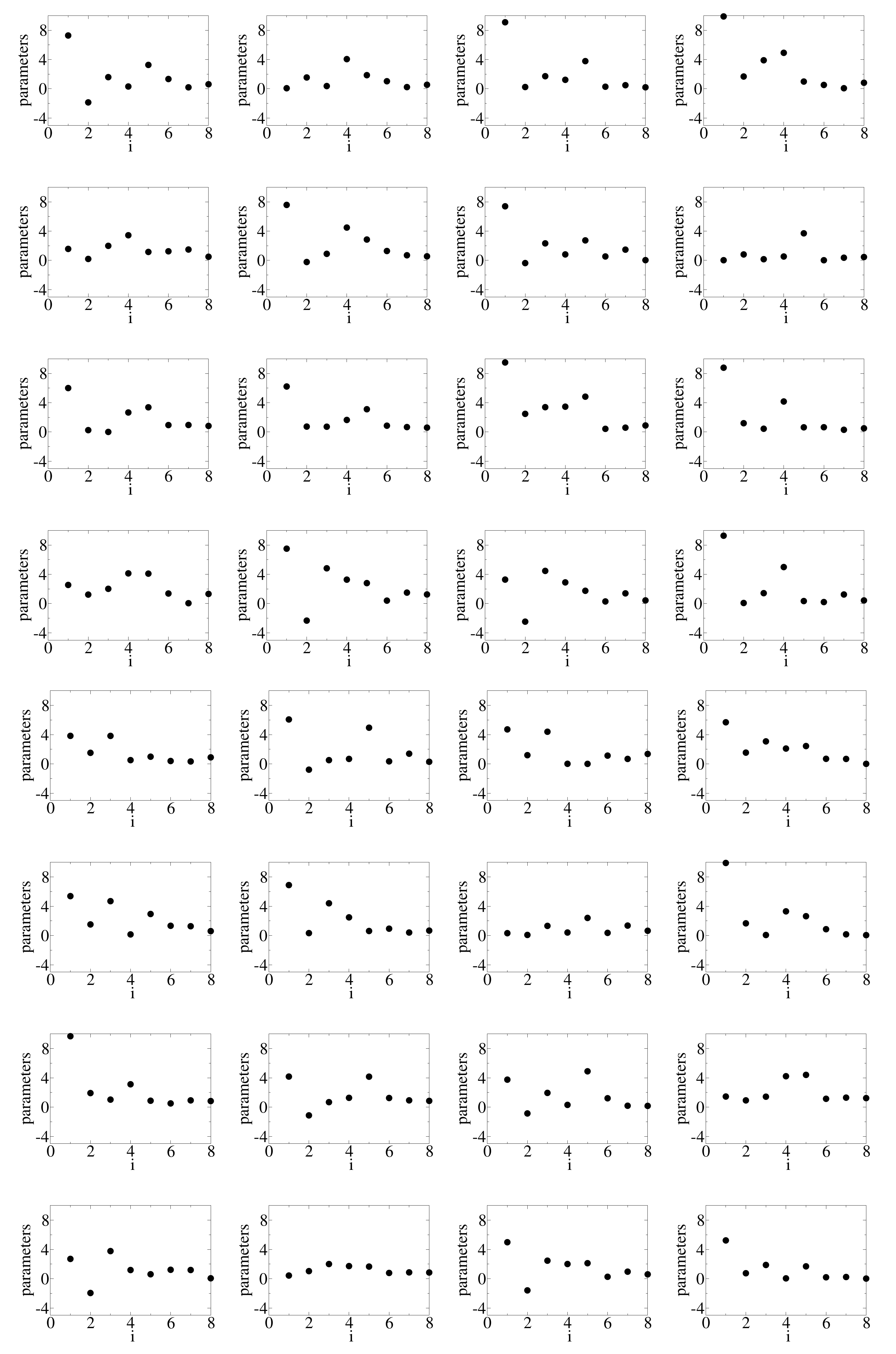
In
Figure 3, we show the spectral functions corresponding to the same 32 samples used in
Figure 2. Both the results from the direct numerical calculation based on the Lanczos method and recurrence relations and those predicted by the neural network are plotted. They basically overlap each other. There is a slight difference for the range of energies where the spectral function is nearly zero. This is perhaps due to the incomplete cancellation among the expansion terms at different orders. An improvement may be attainable if we consider the correlations of the coefficients for different orders. The input parameters of each of the 32 samples are plotted in
Figure 4.
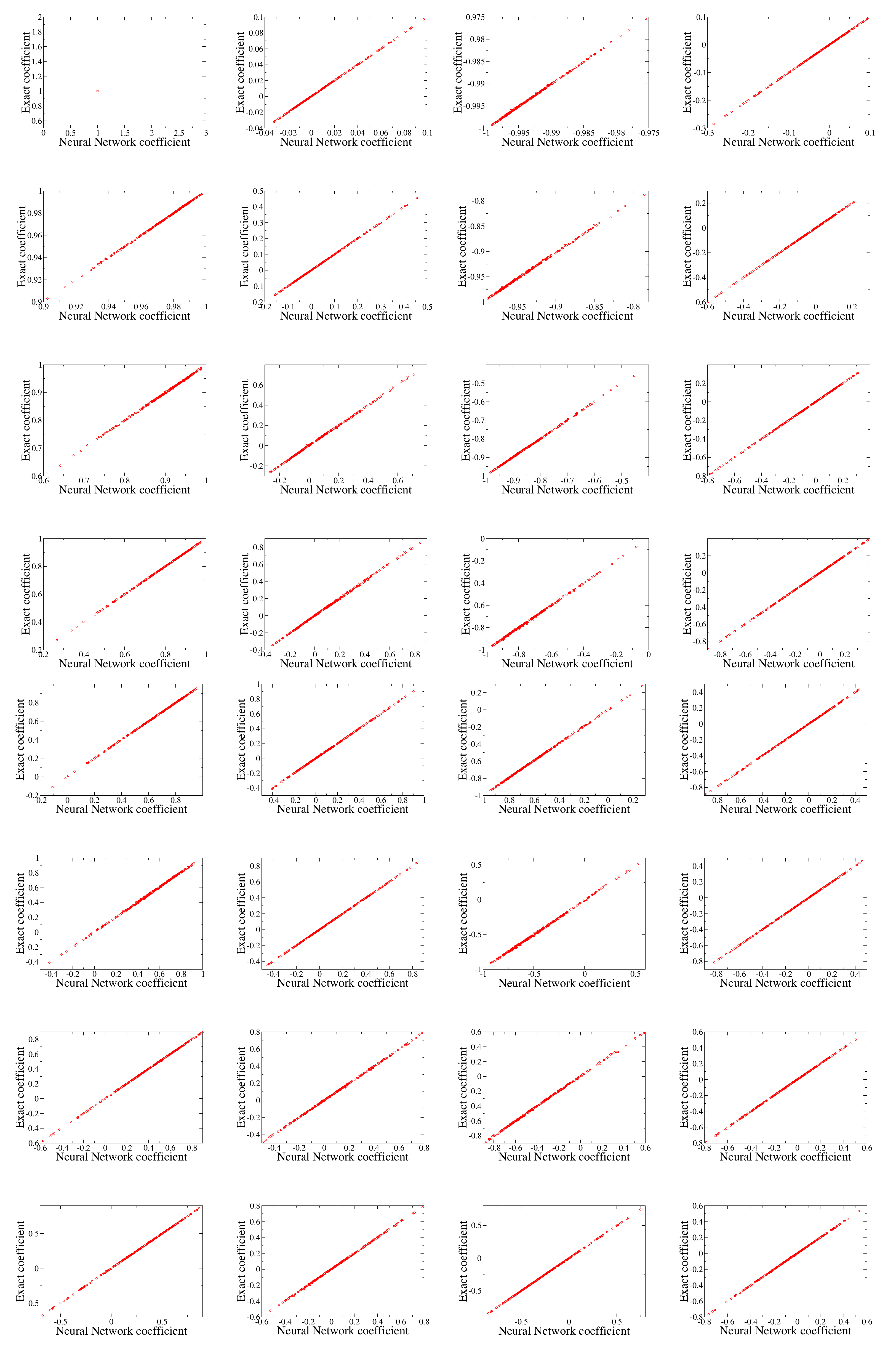
Evidence of the capability of the neural network approach can be seen in
Figure 5 where we plot the comparison of the first 32 expansion coefficients obtained by the direct numerical calculation and the neural network prediction. We find that two methods give very close results for the 1000 testing samples we consider. Please be reminded that 5000 samples are used for training. All the 1000 testing samples exhibit a linear trend. This clearly shows that a neural network is capable of providing a good prediction. There were no exceptional outliers among the 1000 testing samples we tested.
6. Conclusions
We demonstrate that the supervised machine learning approach, specifically the neural network method, can be utilized as a solver for small quantum interacting clusters. This could be potentially useful for the statistical DMFT or the typical medium theory for which a large number of impurity problems have to be solved to perform the disorder averaging [
29,
30,
31,
32,
33,
36]. The main strategy is to devise a finite number of variables as the feature vector and the label for the supervised machine learning method. In line with the exact diagonalization method for the single impurity Anderson model, the feature vector is represented by the hoppings and the energies of the lattice model. The output we consider, the spectral function, is represented in terms of Chebyshev polynomials with a damping kernel. The labels are then the coefficients of the expansion. By comparing the coefficients directly calculated by the Lanczos method and the recurrence relation with the ones by the neural network, we find the agreement between these two methods is very good. Notably, among the 1000 samples we tested, there is no exceptional outlier. They all have a good agreement with the results of the numerical method.
For a simple impurity problem, the present method may not have an obvious benefit, as a rather large pool of samples have to be generated for training purposes. The situation is completely different for the study of disorder models, such as those being studied by the typical medium theory, where the present method has a clear advantage. Once the neural network is trained, the calculations are computationally inexpensive. For systems in which disorder averaging is required, this method can beat most if not all other numerical methods in term of efficiency. Moreover, the present approach is rather easy to be generalized for more complicated models, such as the few impurities models required in the dynamical cluster approximation. In addition, this method can be easily adapted to the matrix product basis proposed for the kernel polynomial expansion [
48,
53].
The range of parameters we choose in the present study covers the metal insulator transition of the Hubbard model within the single impurity dynamical mean field theory. An interesting question is the validity of the trained neural networks for the parameters well outside the range of the training data. We expect that the results could deteriorate without additional training data.
The size of the bath we choose in the present study is . This choice is somewhat arbitrary, for more accurate results for the single impurity problem a larger number of bath sites is preferred. The computational time required to generate the training set scales exponentially with the number of bath sites; however the computational time required to train the neural networks only scales as the third power with the number of bath sites. A larger number of bath sites should pose no problem for the present approach.
The ideas presented in this paper are rather generic. They can be generalized to the solutions by different solvers. For example, this approach can be adapted to Quantum Monte Carlo results as long as they can be represented in some kind of series expansion [
54,
55]. Our approach can also be adapted to predict the the coefficients of the coupled cluster theory [
19,
20].
Author Contributions
Conceptualization, K.-M.T.; Data curation, K.-M.T.; Formal analysis, J.M.; Funding acquisition, K.-M.T. and J.M.; Investigation, K.-M.T.; Methodology, K.-M.T., N.W., S.K. and Y.Z.; Project administration, J.M.; Supervision, J.M.; Writing—original draft, K.-M.T.; Writing—review & editing, J.M., N.W., S.K. and Y.Z. All authors have read and agreed to the published version of the manuscript.
Funding
This work is funded by the NSF Materials Theory grant DMR-1728457. Additional support was provided by NSF-EP- SCoR award OIA-1541079 (N.W. and K.-M.T.) and by the U.S. Department of Energy, Office of Science, Office of Basic Energy Sciences under Award No. DE-SC0017861 (Y.Z., J.M.).
Institutional Review Board Statement
Not applicable.
Informed Consent Statement
Not applicable.
Data Availability Statement
Correspondence and requests for data should be addressed to K.-M.T.
Acknowledgments
This work used the high performance computational resources provided by the Louisiana Optical Network Initiative (
http://www.loni.org) and HPC@LSU computing, accessed from 1 January 2019 to 1 January 2022.
Conflicts of Interest
The authors declare no conflict of interest.
References
- Kondo, J. Resistance Minimum in Dilute Magnetic Alloys. Prog. Theor. Phys. 1964, 32, 37–49. [Google Scholar] [CrossRef]
- Anderson, P.W. A poor man’s derivation of scaling laws for the Kondo problem. J. Phys. C Solid State Phys. 1970, 3, 2436–2441. [Google Scholar] [CrossRef]
- Wilson, K.G. The renormalization group: Critical phenomena and the Kondo problem. Rev. Mod. Phys. 1975, 47, 773–840. [Google Scholar] [CrossRef]
- Müller-Hartmann, E. The Hubbard model at high dimensions: Some exact results and weak coupling theory. Z. Phys. B 1989, 76, 211–217. [Google Scholar] [CrossRef]
- Müller-Hartmann, E. Correlated fermions on a lattice in high dimensions. Z. Phys. B 1989, 74, 507–512. [Google Scholar] [CrossRef]
- Metzner, W.; Vollhardt, D. Correlated Lattice Fermions in d=∞ Dimensions. Phys. Rev. Lett. 1989, 62, 324–327. [Google Scholar] [CrossRef] [PubMed]
- Bray, A.J.; Moore, M.A. Replica theory of quantum spin glasses. J. Phys. C Solid State Phys. 1980, 13, L655–L660. [Google Scholar] [CrossRef]
- Georges, A.; Kotliar, G.; Krauth, W.; Rozenberg, M.J. Dynamical mean-field theory of strongly correlated fermion systems and the limit of infinite dimensions. Rev. Mod. Phys. 1996, 68, 13–125. [Google Scholar] [CrossRef]
- Hettler, M.H.; Mukherjee, M.; Jarrell, M.; Krishnamurthy, H.R. Dynamical cluster approximation: Nonlocal dynamics of correlated electron systems. Phys. Rev. B 2000, 61, 12739–12756. [Google Scholar] [CrossRef]
- Biroli, G.; Kotliar, G. Cluster methods for strongly correlated electron systems. Phys. Rev. B 2002, 65, 155112. [Google Scholar] [CrossRef] [Green Version]
- Maier, T.; Jarrell, M.; Pruschke, T.; Hettler, M.H. Quantum cluster theories. Rev. Mod. Phys. 2005, 77, 1027–1080. [Google Scholar] [CrossRef]
- Kotliar, G.; Savrasov, S.Y.; Haule, K.; Oudovenko, V.S.; Parcollet, O.; Marianetti, C.A. Electronic structure calculations with dynamical mean-field theory. Rev. Mod. Phys. 2006, 78, 865–951. [Google Scholar] [CrossRef]
- Kajueter, H.; Kotliar, G. New Iterative Perturbation Scheme for Lattice Models with Arbitrary Filling. Phys. Rev. Lett. 1996, 77, 131–134. [Google Scholar] [CrossRef]
- Logan, D.E.; Glossop, M.T. A local moment approach to magnetic impurities in gapless Fermi systems. J. Phys. Condens. Matter 2000, 12, 985–1028. [Google Scholar] [CrossRef]
- Caffarel, M.; Krauth, W. Exact diagonalization approach to correlated fermions in infinite dimensions: Mott transition and superconductivity. Phys. Rev. Lett. 1994, 72, 1545–1548. [Google Scholar] [CrossRef] [PubMed]
- Krishna-Murthy, H.R.; Wilkins, J.W.; Wilson, K.G. Renormalization-group approach to the Anderson model of dilute magnetic alloys. I. Static properties for the symmetric case. Phys. Rev. B 1980, 21, 1003–1043. [Google Scholar] [CrossRef]
- Núñez Fernández, Y.; Hallberg, K. Solving the Multi-site and Multi-orbital Dynamical Mean Field Theory Using Density Matrix Renormalization. Front. Phys. 2018, 6, 13. [Google Scholar] [CrossRef]
- Ganahl, M.; Aichhorn, M.; Evertz, H.G.; Thunström, P.; Held, K.; Verstraete, F. Efficient DMFT impurity solver using real-time dynamics with matrix product states. Phys. Rev. B 2015, 92, 155132. [Google Scholar] [CrossRef]
- Zhu, T.; Jiménez-Hoyos, C.A.; McClain, J.; Berkelbach, T.C.; Chan, G.K.L. Coupled-cluster impurity solvers for dynamical mean-field theory. Phys. Rev. B 2019, 100, 115154. [Google Scholar] [CrossRef]
- Shee, A.; Zgid, D. Coupled Cluster as an impurity solver for Green’s function embedding methods. arXiv 2019, arXiv:1906.04079. [Google Scholar] [CrossRef] [Green Version]
- Hirsch, J.E.; Fye, R.M. Monte Carlo Method for Magnetic Impurities in Metals. Phys. Rev. Lett. 1986, 56, 2521–2524. [Google Scholar] [CrossRef] [PubMed]
- Hirsch, J.E. Discrete Hubbard-Stratonovich transformation for fermion lattice models. Phys. Rev. B 1983, 28, 4059–4061. [Google Scholar] [CrossRef]
- Rubtsov, A.N.; Savkin, V.V.; Lichtenstein, A.I. Continuous-time quantum Monte Carlo method for fermions. Phys. Rev. B 2005, 72, 35122. [Google Scholar] [CrossRef]
- Werner, P.; Millis, A.J. Hybridization expansion impurity solver: General formulation and application to Kondo lattice and two-orbital models. Phys. Rev. B 2006, 74, 155107. [Google Scholar] [CrossRef]
- Carrasquilla, J.; Melko, R.G. Machine learning phases of matter. Nat. Phys. 2017, 13, 431–434. [Google Scholar] [CrossRef]
- Huang, L.; Wang, L. Accelerated Monte Carlo simulations with restricted Boltzmann machines. Phys. Rev. B 2017, 95, 35105. [Google Scholar] [CrossRef]
- Wang, L. Discovering phase transitions with unsupervised learning. Phys. Rev. B 2016, 94, 195105. [Google Scholar] [CrossRef]
- Arsenault, L.F.; Lopez-Bezanilla, A.; von Lilienfeld, O.A.; Millis, A.J. Machine learning for many-body physics: The case of the Anderson impurity model. Phys. Rev. B 2014, 90, 155136. [Google Scholar] [CrossRef]
- Dobrosavljević, V.; Pastor, A.A.; Nikolić, B.K. Typical medium theory of Anderson localization: A local order parameter approach to strong-disorder effects. EPL 2003, 62, 76–82. [Google Scholar] [CrossRef]
- Ekuma, C.E.; Terletska, H.; Tam, K.M.; Meng, Z.Y.; Moreno, J.; Jarrell, M. Typical medium dynamical cluster approximation for the study of Anderson localization in three dimensions. Phys. Rev. B 2014, 89, 81107. [Google Scholar] [CrossRef] [Green Version]
- Terletska, H.; Zhang, Y.; Chioncel, L.; Vollhardt, D.; Jarrell, M. Typical-medium multiple-scattering theory for disordered systems with Anderson localization. Phys. Rev. B 2017, 95, 134204. [Google Scholar] [CrossRef]
- Zhang, Y.; Terletska, H.; Moore, C.; Ekuma, C.; Tam, K.M.; Berlijn, T.; Ku, W.; Moreno, J.; Jarrell, M. Study of multiband disordered systems using the typical medium dynamical cluster approximation. Phys. Rev. B 2015, 92, 205111. [Google Scholar] [CrossRef]
- Dobrosavljević, V.; Kotliar, G. Dynamical mean–field studies of metal–insulator transitions. Philos. Trans. R. Soc. London. Ser. A Math. Phys. Eng. Sci. 1998, 356, 57–74. [Google Scholar] [CrossRef]
- Terletska, H.; Zhang, Y.; Tam, K.M.; Berlijn, T.; Chioncel, L.; Vidhyadhiraja, N.; Jarrell, M. Systematic quantum cluster typical medium method for the study of localization in strongly disordered electronic systems. Appl. Sci. 2018, 8, 2401. [Google Scholar] [CrossRef]
- Zhang, Y.; Nelson, R.; Siddiqui, E.; Tam, K.M.; Yu, U.; Berlijn, T.; Ku, W.; Vidhyadhiraja, N.S.; Moreno, J.; Jarrell, M. Generalized multiband typical medium dynamical cluster approximation: Application to (Ga, Mn)N. Phys. Rev. B 2016, 94, 224208. [Google Scholar] [CrossRef]
- Ekuma, C.E.; Yang, S.X.; Terletska, H.; Tam, K.M.; Vidhyadhiraja, N.S.; Moreno, J.; Jarrell, M. Metal-insulator transition in a weakly interacting disordered electron system. Phys. Rev. B 2015, 92, 201114. [Google Scholar] [CrossRef]
- Ulmke, M.; Janiš, V.; Vollhardt, D. Anderson-Hubbard model in infinite dimensions. Phys. Rev. B 1995, 51, 10411–10426. [Google Scholar] [CrossRef]
- Semmler, D.; Byczuk, K.; Hofstetter, W. Anderson-Hubbard model with box disorder: Statistical dynamical mean-field theory investigation. Phys. Rev. B 2011, 84, 115113. [Google Scholar] [CrossRef]
- Byczuk, K.; Hofstetter, W.; Vollhardt, D. Mott-Hubbard Transition versus Anderson Localization in Correlated Electron Systems with Disorder. Phys. Rev. Lett. 2005, 94, 056404. [Google Scholar] [CrossRef]
- de Vega, I.; Schollwöck, U.; Wolf, F.A. How to discretize a quantum bath for real-time evolution. Phys. Rev. B 2015, 92, 155126. [Google Scholar] [CrossRef] [Green Version]
- Liebsch, A.; Ishida, H. Temperature and bath size in exact diagonalization dynamical mean field theory. J. Phys. Soc. Jpn. 2011, 24, 53201. [Google Scholar] [CrossRef] [PubMed]
- Medvedeva, D.; Iskakov, S.; Krien, F.; Mazurenko, V.V.; Lichtenstein, A.I. Exact diagonalization solver for extended dynamical mean-field theory. Phys. Rev. B 2017, 96, 235149. [Google Scholar] [CrossRef]
- Nagai, Y.; Shinaoka, H. Smooth Self-energy in the Exact-diagonalization-based Dynamical Mean-field Theory: Intermediate-representation Filtering Approach. J. Phys. Soc. Jpn. 2019, 88, 064004. [Google Scholar] [CrossRef]
- Sénéchal, D. Bath optimization in the cellular dynamical mean-field theory. Phys. Rev. B 2010, 81, 235125. [Google Scholar] [CrossRef]
- Weiße, A.; Wellein, G.; Alvermann, A.; Fehske, H. The kernel polynomial method. Rev. Mod. Phys. 2006, 78, 275–306. [Google Scholar] [CrossRef]
- Lin, H.Q. Exact diagonalization of quantum-spin models. Phys. Rev. B 1990, 42, 6561–6567. [Google Scholar] [CrossRef]
- Lin, H.; Gubernatis, J. Exact Diagonalization Methods for Quantum Systems. Comput. Phys. 1993, 7, 400–407. [Google Scholar] [CrossRef]
- Wolf, F.A.; McCulloch, I.P.; Parcollet, O.; Schollwöck, U. Chebyshev matrix product state impurity solver for dynamical mean-field theory. Phys. Rev. B 2014, 90, 115124. [Google Scholar] [CrossRef]
- Silver, R.; Röder, H. Densities of states of mega-dimensional Hamiltonian matrices. Int. Mod. Phys. C 1994, 5, 735–753. [Google Scholar] [CrossRef]
- Silver, R.; Röder, H.; Voter, A.; Kress, J. Kernel Polynomial Approximations for Densities of States and Spectral Functions. J. Comput. Phys. 1996, 124, 115–130. [Google Scholar] [CrossRef]
- Silver, R.N.; Röder, H. Calculation of densities of states and spectral functions by Chebyshev recursion and maximum entropy. Phys. Rev. E 1997, 56, 4822–4829. [Google Scholar] [CrossRef]
- Alvermann, A.; Fehske, H. Chebyshev approach to quantum systems coupled to a bath. Phys. Rev. B 2008, 77, 45125. [Google Scholar] [CrossRef]
- Wolf, F.A.; Justiniano, J.A.; McCulloch, I.P.; Schollwöck, U. Spectral functions and time evolution from the Chebyshev recursion. Phys. Rev. B 2015, 91, 115144. [Google Scholar] [CrossRef]
- Huang, L. Kernel polynomial representation for imaginary-time Green’s functions in continuous-time quantum Monte Carlo impurity solver. Chin. Phys. B 2016, 25, 117101. [Google Scholar] [CrossRef]
- Boehnke, L.; Hafermann, H.; Ferrero, M.; Lechermann, F.; Parcollet, O. Orthogonal polynomial representation of imaginary-time Green’s functions. Phys. Rev. B 2011, 84, 75145. [Google Scholar] [CrossRef] [Green Version]
| Publisher’s Note: MDPI stays neutral with regard to jurisdictional claims in published maps and institutional affiliations. |
© 2022 by the authors. Licensee MDPI, Basel, Switzerland. This article is an open access article distributed under the terms and conditions of the Creative Commons Attribution (CC BY) license (https://creativecommons.org/licenses/by/4.0/).


