We perform several numerical experiments to evaluate the flow stability in the down-flow and up-flow reactor. By using simplified gas compositions in the run lines, we propose a novel approach for the analysis of the gas flow stability in vertical HVPE reactors. Starting from the laminar N
flow, we add for the growth reasonable amounts of NH
or GaCl/H
in the ORL or IRL, respectively, and investigate its effect on the stability of the gas flow. We base our investigations on the stability in different fluid regimes on the molar Grashof
, the thermal Grashof
and the Reynolds numbers
. The definition of the respective reference values are given in
Table 1. Therefore, it should be mentioned at this point that the thermal Grashof number
is constant in all simulations because the thermal boundary conditions are not changed, i.e.,
.
The reference velocity
is defined as the area-averaged mean velocity at the inlets, i.e.,
where
denotes the surface of the inlet
. In order to define the inlet velocities,
, we consider reference inlet velocities relative to the inlet velocity
m/s, where
denotes the up-flow reactor and
denotes the down-flow reactor. Then, in order to vary the Reynolds number, we define the inlet velocities by scaling the reference values by a constant factor. According to (
16), we allow negative and positive Reynolds numbers in (
12) to refer to the down-flow and up-flow reactor, respectively.
Furthermore, we define
in terms of the possible four different molar masses at the inlets. Due to the axial symmetric reactor geometry, we obtain three different possible values, i.e.,
We use each of the above definitions in the respective simulations. Lastly, we propose a definition of unstable flow behavior. We aim for a criterion that reflects the occurrence of vortices and recirculizations in the reactor.
In other words, the function defined in (
19) identifies regions where the flow velocity vector deviates more then
from its intended direction, which in the up-flow case is against the vector of gravity and in the down-flow case along the vector of gravity. Accordingly, the function
defined in (
18) is able to identify if instabilities occur over a defined time interval in the specified domain
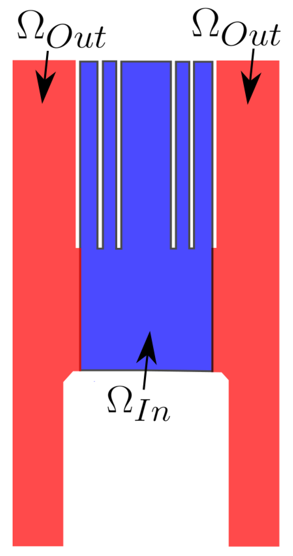
. In order to distinguish different flow phenomena, we split the reactor
in an outer part and in an inner part, denoted by
and
, respectively, with
. In
Figure 2, we depict the definition of
and
for the down-flow reactor. The definition for the up-flow reactor is analogous following
Figure 1.
4.1. Variation of NH in ORL
First we investigated the variation of
in the ORL for the up-flow and the down-flow reactor. Apart from the ammonia in the ORL, only
was used in all the other gas lines. Following (
17), we used
in (
14) to define the molar Grashof number. Consequently, from the molar masses of
and
, we found that
, and therefore,
in this simulation series.
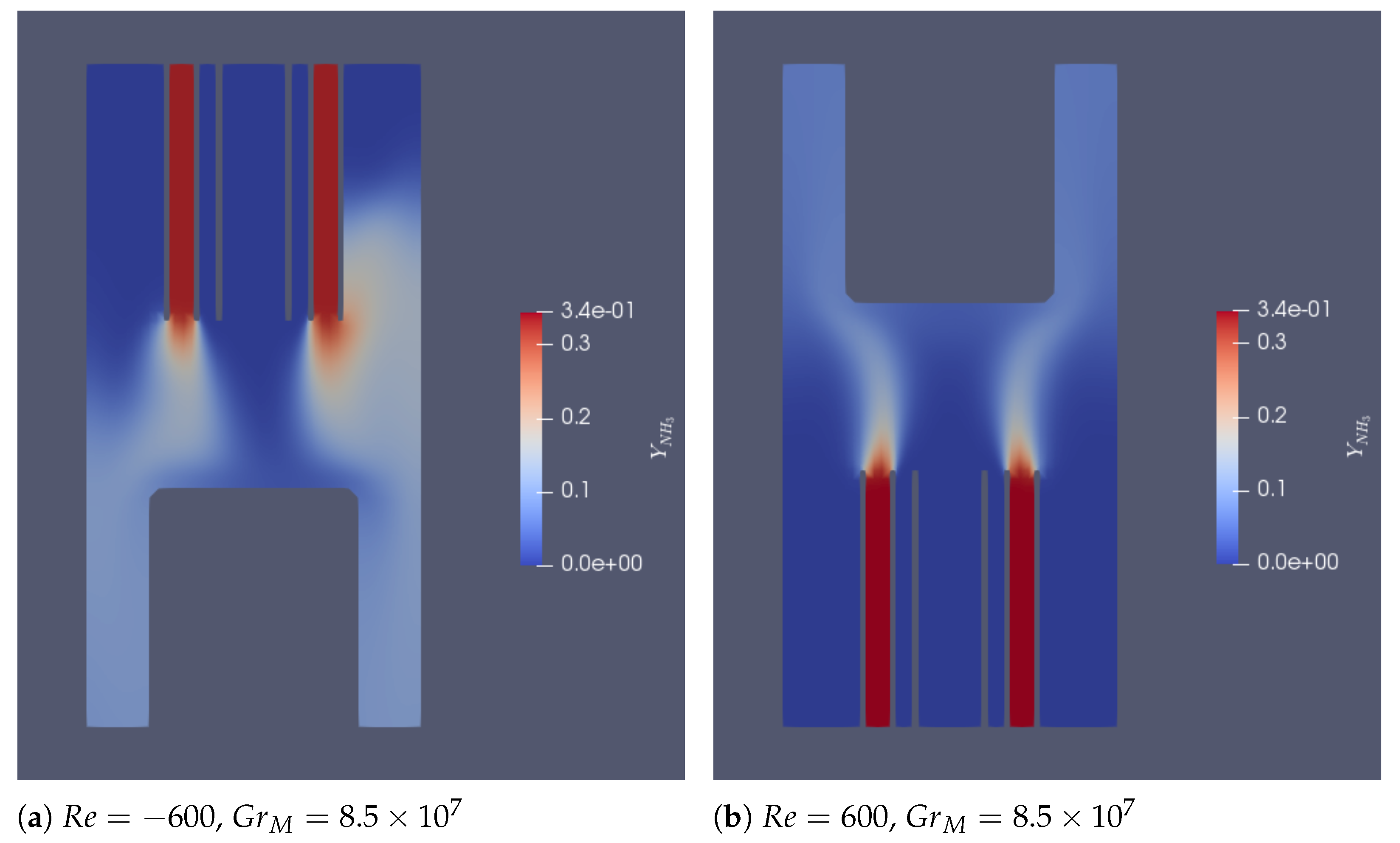
In
Figure 3, snapshots of the distribution of
in a vertical cut of both the up-flow and the down-flow reactor for
and
are shown. It is obvious that the gas flow behaves differently for the two setups. In the up-flow configuration, the distribution of
is symmetric and follows the general direction of the flow, while in the down-flow configuration, the ammonia also flows into the outer and upper part of the reactor.
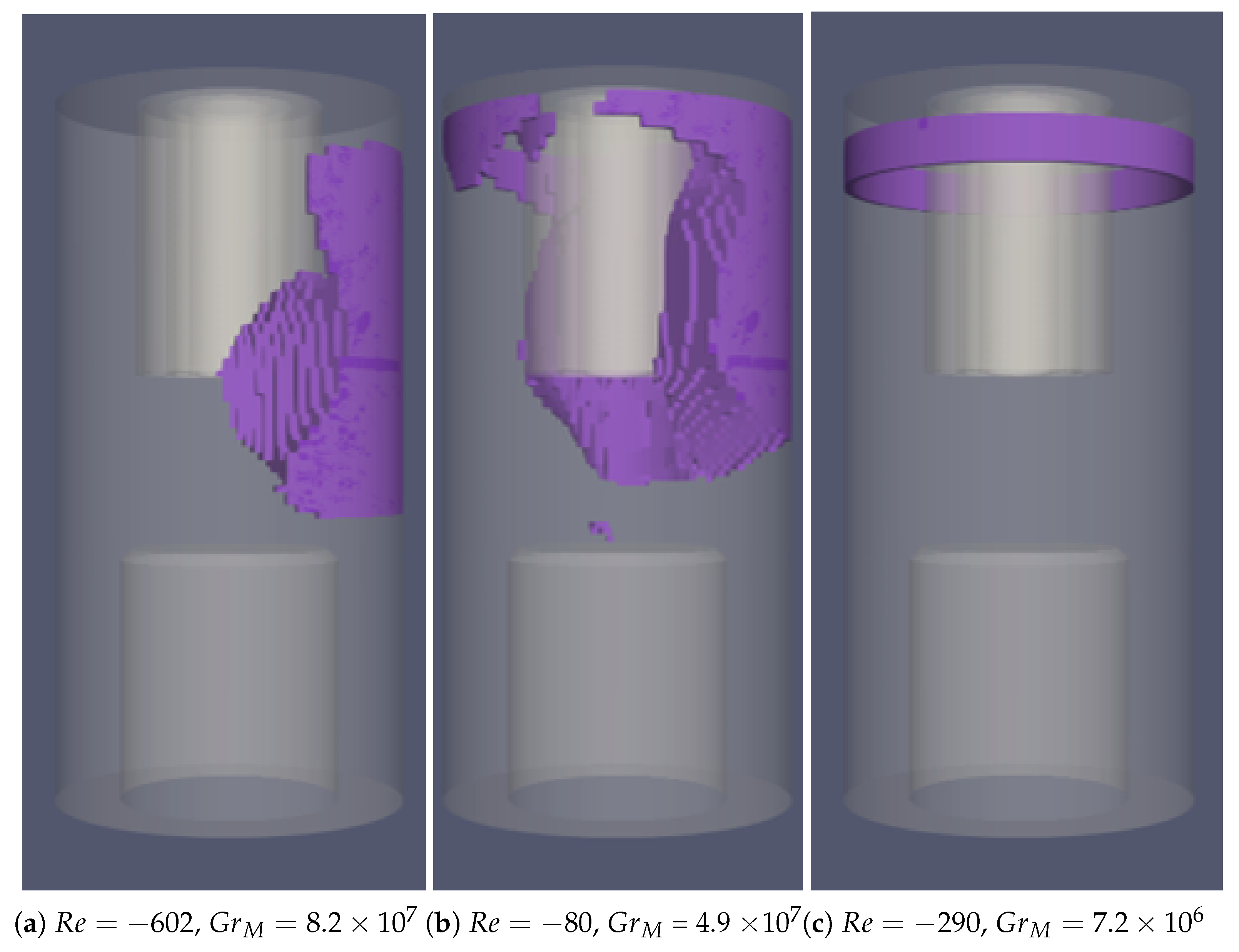
We performed multiple simulations at different Reynolds and Grashof numbers and checked for the occurrence of instabilities.
Figure 4 shows exemplarily typical regions where the instabilities in the down-flow and up-flow configuration occur for different Re and Gr numbers.
In
Figure 4a, the instabilities are present mainly in the outer part of the growth zone below and above the position of the gas nozzles for the down-flow reactor, while in
Figure 4c, the instabilities are located exclusively in the upper part between the SWP gas line and the reactor wall. The most critical disturbance for crystal growth of GaN in the down-flow configuration is shown in
Figure 4b as the instabilities occur directly in the vicinity of the growing crystal in the inner part of the growth zone as well as in the outer part.
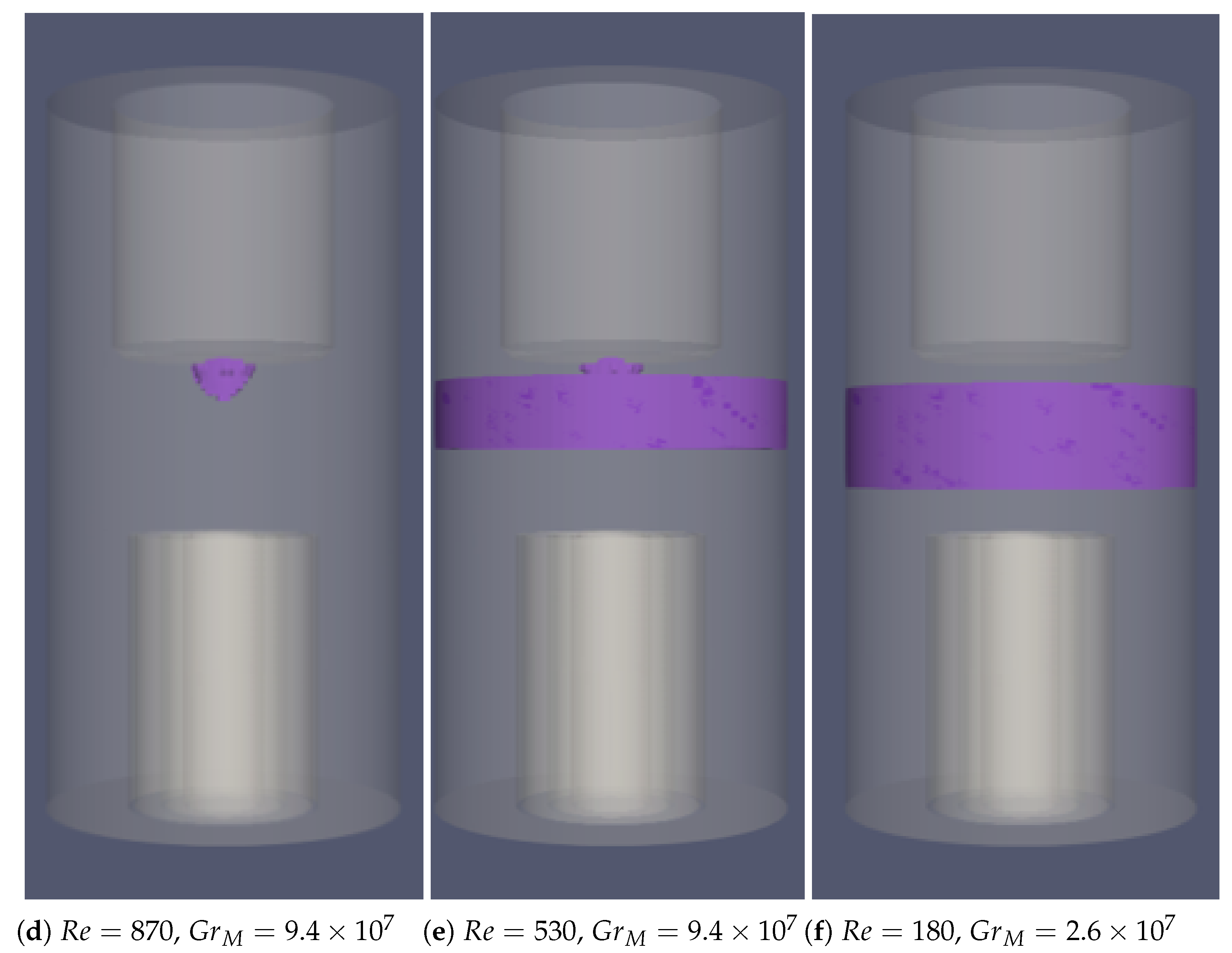
Typical locations of the instabilities in the up-flow configuration are shown in
Figure 4d–f. Again, we can distinguish less harmful cases, where the instabilities occur only in the outer part (see
Figure 4f) and more severe cases, where the instabilities are located close to the growing crystal in the inner part (see
Figure 4d) or even in the inner and outer part (see
Figure 4e).
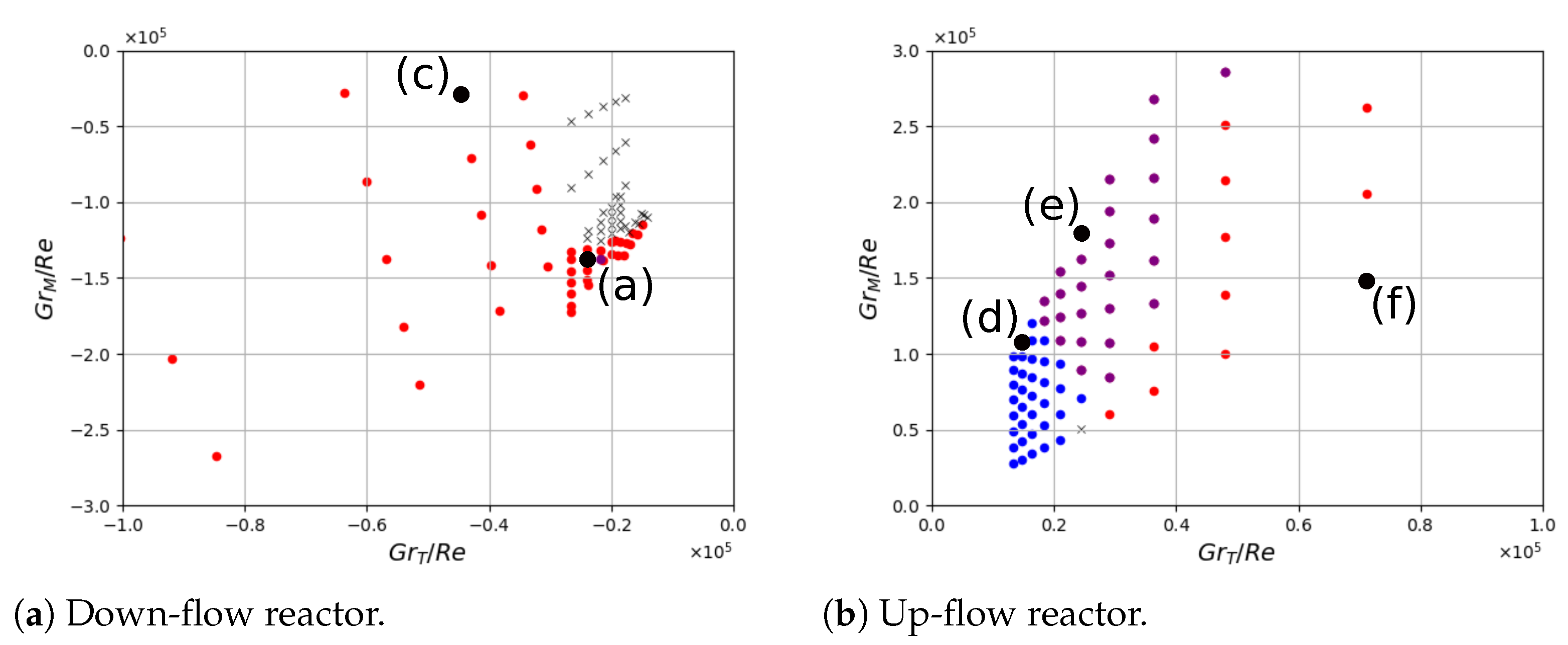
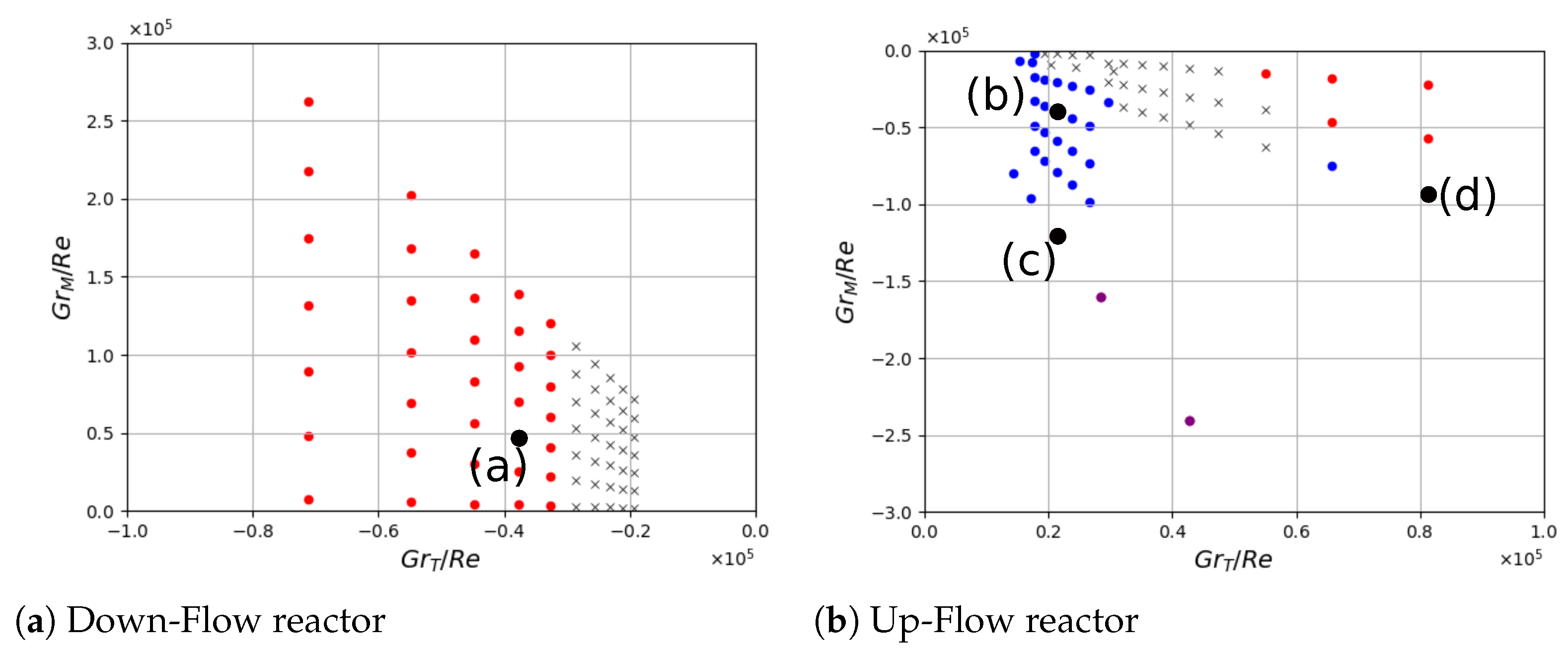
Figure 5 summarizes the results of the variation of NH
in the ORL for the down-flow (see
Figure 5a) and up-flow (see
Figure 5b) configurations in the form of a stability diagram in the
/
over
/
parameter space. For the down-flow reactor, it is obvious that for
and independent of the
ratio, the flow is always unstable and the instabilities occur mainly in the outer parts; see, for example
Figure 4c. For
and
, the flow is stable without any disturbance, while the flow becomes unstable again for
and
with disturbances in the outer part of the growth zone; see
Figure 4a.
Figure 4b refers to a fluid regime outside any of the previous described stability boundaries for
and
. Moreover, we find that for a given
, the stability region can be extended by increasing the Re number.
The stability regions for the up-flow reactor behave differently from the down-flow configuration, as shown in
Figure 5b. Instabilities in the outer part of the reactor are found only typically for
; compare
Figure 4f. This is slightly higher than in the down-flow configuration, where the transition took place at
. Opposite to the down-flow reactor, no stability region exists in the up-flow configuration, and the flow is always unstable for
, where instabilities occur mostly in the inner part of the reactor; see
Figure 4d. Thereby, it is obvious that there exists a transition region between
. Within this region, instabilities occur in the inner and outer part; see
Figure 4e.
In the next section, we present the results regarding the stability of the flow with respect to a variation of the gas mixture in the IRL.
4.2. Variation of H in IRL
In the second case study, we considered the variation of
in the IRL, where a mixture of GaCl,
and
was used. In all the other lines, only
was applied. We varied the amount of
while keeping
constant until a maximum such that the molar mass of the IRL equaled that of pure
. Following (
17), we use
in (
14) to define the molar Grashof number. Consequently, there was
, and therefore,
in this simulation series.
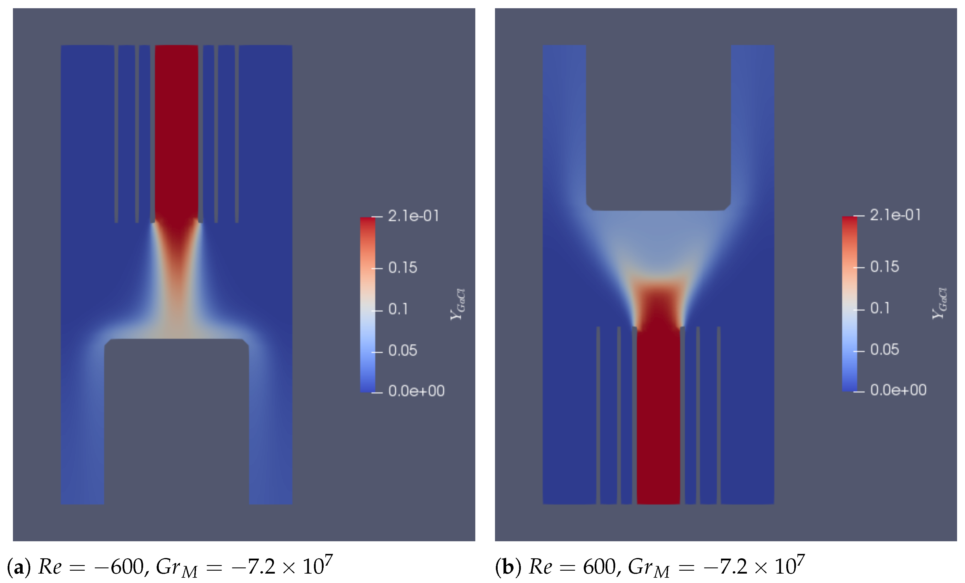
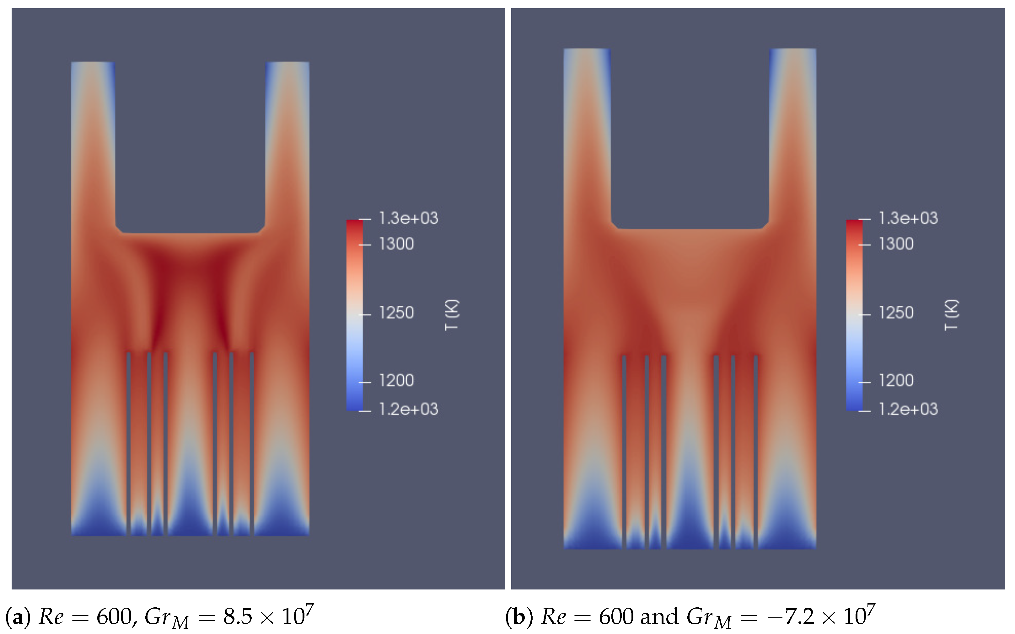
In
Figure 6, snapshots of the distribution of
in a vertical cut of both the up-flow and the down-flow reactors for
and
are shown. Again, the gas flow behaves differently for the two setups. While in the down-flow reactor, the GaCl flows laminarly from the nozzle to the growing crystal, in the up-flow reactor, the GaCl spreads significantly towards the outer part of the reactor after leaving the nozzle.
Again we performed a case study for different Reynolds and Grashof numbers by varying the inlet velocities, and we progressively substituted
by
in the IRL until there was no molar mass gradient.
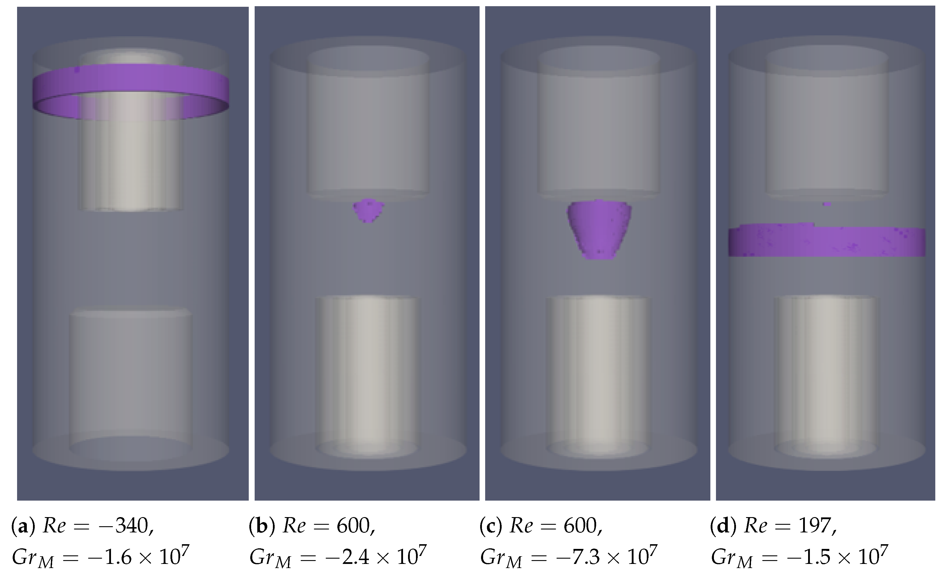
Figure 7 shows exemplary typical regions where the instabilities in the down-flow and up-flow configuration occur for different Re and Gr numbers. In the down-flow reactor, the instabilities occur only in the outer part of the reactor, while for the up-flow configuration, the flow is disturbed in the inner and outer part depending on the Re and Gr numbers.
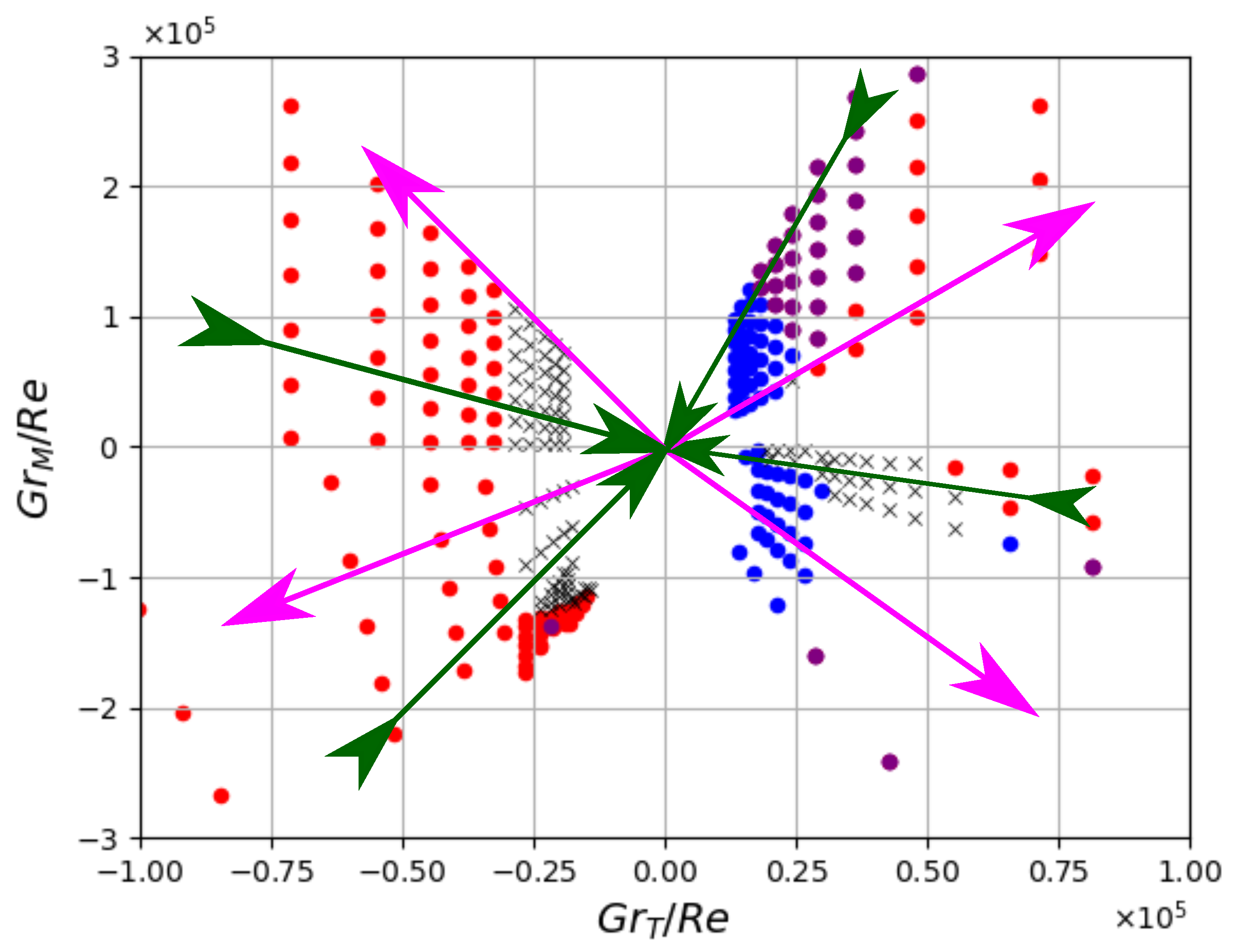
Figure 8 summarizes the results of the variation of H
in the IRL for the down-flow (see
Figure 8a) and up-flow (see
Figure 8b) configurations in the form of a stability diagram in the
over
parameter space. For the down-flow geometry, when the gas mixture in the IRL is varied, there also exists a critical
ratio. For
, the flow is always unstable in the outer part of the growth zone (compare
Figure 7a), while for
, no disturbance of the flow occurs at all in the considered parameter range. Interestingly, the transition takes place almost at the same critical
ratio for a variation of the gas mixture in the IRL as in the case where we varied the gas composition in the ORL. However, in the case of the variation of the gas composition of the ORL, instabilities were also found in the inner part for a high
ratio, which do not exist in the present case.
For the up-flow reactor (see
Figure 8b), there are again three stability regions. For
, instabilities are present mainly in the outer areas (compare
Figure 7d), whereas for
, the flow is disturbed in the inner part close to the growing crystals (compare
Figure 7b). In between, a stable flow regime exists for
.
4.3. Analysis of the Instabilities for the Down-Flow Reactor
In order to find the different causes for the observed flow instabilities, we recall the low Mach number approximation of the vorticity Equation (
15), i.e.,
From Equation (
20), it is obvious that due to the cross-product, not only the magnitude, but also the direction of the molar and thermal gradients with respect to the direction of gravity are important.
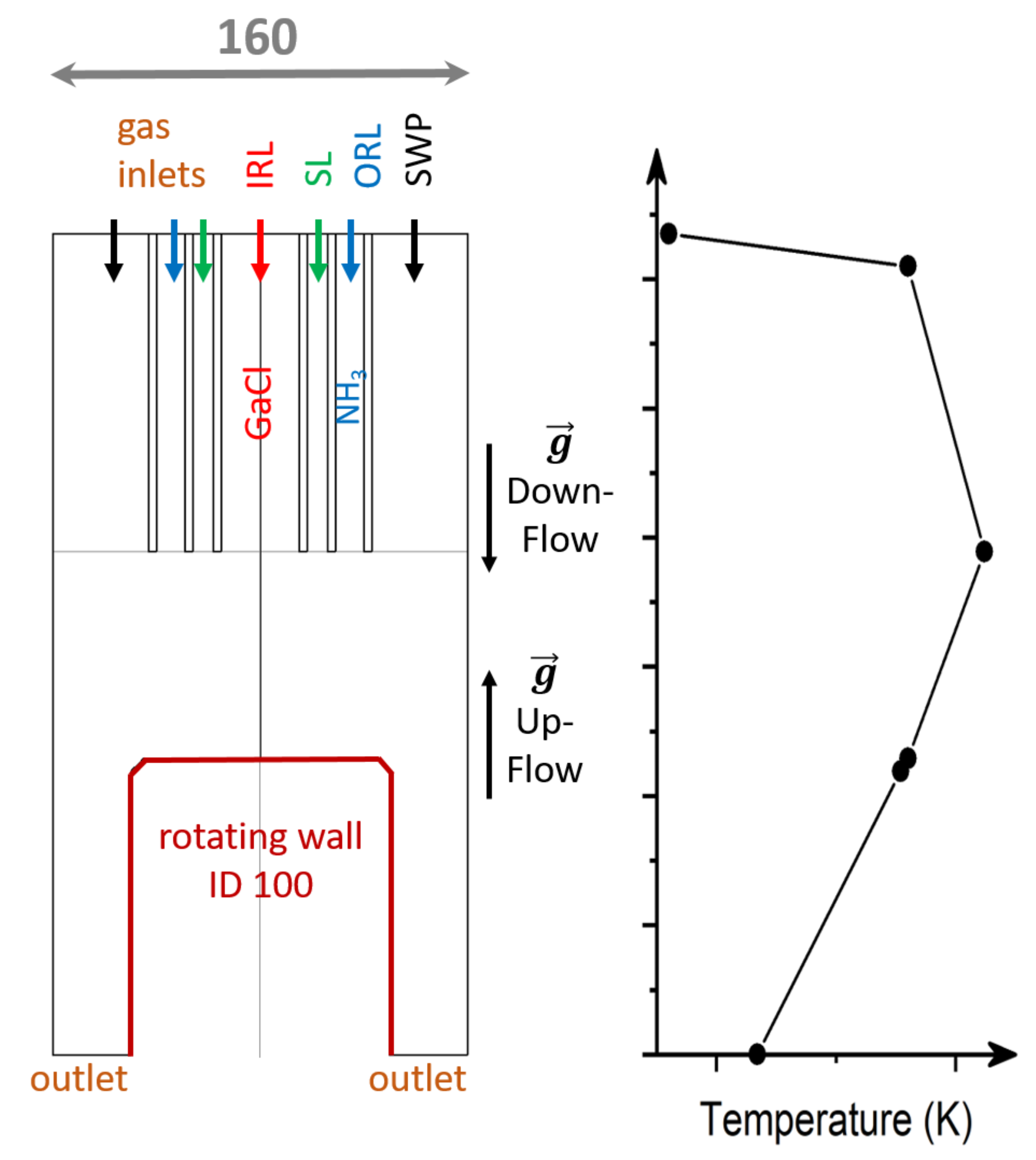
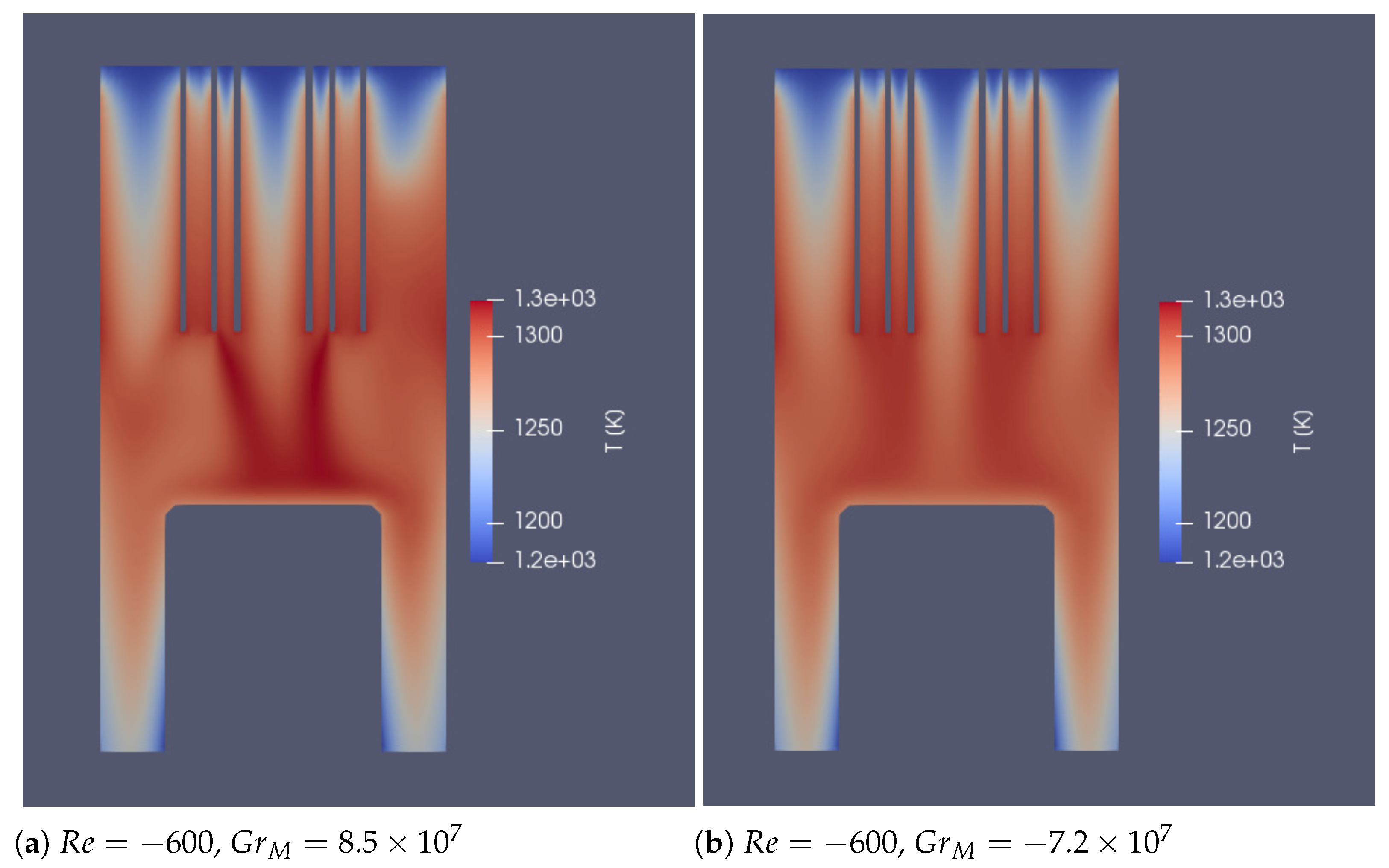
From the thermal boundary conditions shown in
Figure 1, we expect stable thermal conditions for the down-flow configuration above the growing crystal because the gas is hottest at the nozzles and coldest at the crystal, while in the upper reactor part from the gas inlet to the gas outlet at the nozzles, the thermal conditions are considered to be unstable as it is coldest at the inlet and hottest at the outlet. For the up-flow configuration, the thermal conditions are reversed, which means it is unstable under the growing crystal and stable along the gas lines.
In addition, we have to consider that horizontal gradients of the molar mass within the different gas lines exist as well as a horizontal temperature difference within each gas line because cold gas enters the hot reactor, leading to a cold jet in each gas line; see Figures 10 and 12. Since the vector of gravitational acceleration is vertical and for every vector there is , the baroclinic term is expected to depend more on the horizontal variations of the molar mass and the temperature field.
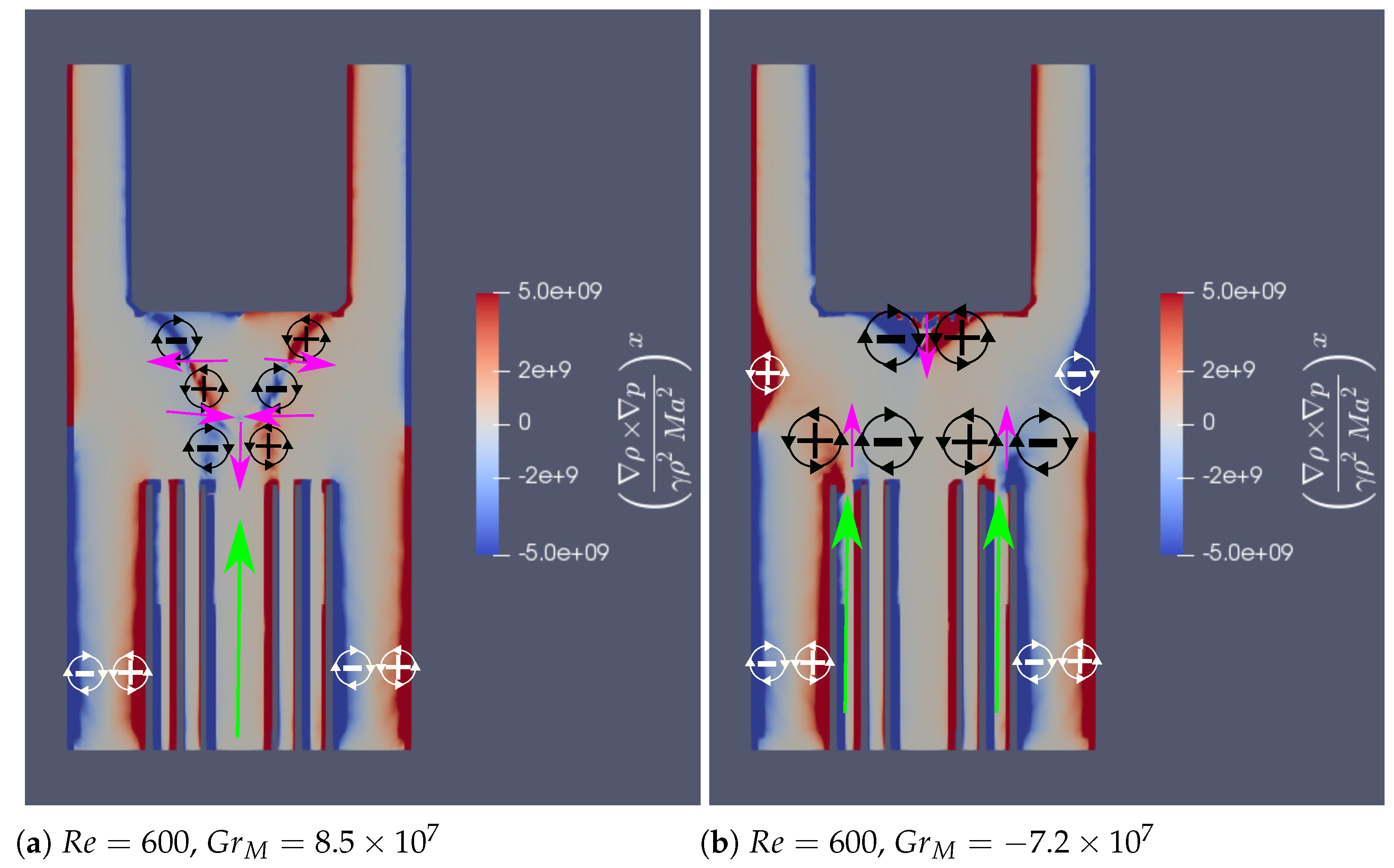
Figure 9 shows the distribution of the x-component of the baroclinic term for the variation of NH
Figure 9a and GaCL/H
Figure 9b in the down-flow reactor. The x-component of the baroclinic term acts as a source for the vorticity component, resembling rotations in the y-z-plane. This is also referred to as baroclinic torque [
28]. The absolute value of the baroclinic torque represents the acceleration of the fluid, while its sign indicates whether the torque is in the positive (counterclockwise) or negative (clockwise) direction.
We start our analysis by identifying regions in the reactor that show a large amount of baroclinicity. For both cases in
Figure 9, we find baroclinic torque to be active at the outer walls of the reactor and beneath the nozzle outlet between the ORL and the SWP, where NH
is varied in the ORL, and between the IRL and the SL, where H
is changed in the IRL.
In the case of the NH
, in the ORL, the baroclinic torque accelerates the gas against its intended flow direction (see
Figure 9a), reducing the vertical fluid velocity beneath the nozzle and transporting NH
towards the outer part of the reactor. Therefore, instabilities in the outer part of the reactor (compare
Figure 4a), and in the inner and outer part (compare
Figure 4b), can be triggered with an increase in
. The approximation of the baroclinic term in (
13) lets us conclude that higher fluid velocities, i.e., higher Re numbers, might suppress the rising of NH
in the outer part of the reactor, as can also be seen in
Figure 5a, since with higher fluid velocities, one moves on rays towards the origin in the plot.
On the other hand, in the case of GaCl in the IRL, the baroclinic torque accelerates the gas along its intended flow direction, leading to a stable flow pattern in terms of the dependence on the molar mass gradients. This is further underlined by the results in the
Figure 7 and
Figure 8a, as no instabilities in the inner part of the reactor above the growing crystal are observed.
Next, we analyze the baroclinicity at the outer reactor walls. The baroclinic torque shown by the white circles in
Figure 9 has the same direction for both cases, variation of NH
in the ORL (see
Figure 9a) and variation of GaCl/H
ratio in IRL (see
Figure 9b). It is expected that the baroclinic torque accelerates the gas towards the reactor side wall, respectively, the quartz cylinder separating the SWP from the ORL, which will promote the occurrence of instabilities. From
Figure 10, it is clear that this baroclinic torque at the outer walls is induced by horizontal thermal gradients. These horizontal gradients originate from the heating of the gas through the reactor wall while flowing downwards towards the mixing zone. This hypothesis is supported by the results from
Figure 4 and
Figure 7, where we find that the instabilities occur in both cases, i.e., variation of NH
in the ORL and variation of GaCl/H
ratio in IRL, at the same critical
ratio, i.e.,
. However, from a practical point of view. it can be stated that usually in real crystal growth experiments, the Reynolds number is relatively high and therefore should be not in a regime where these instabilities driven by horizontal temperature gradients occur.
4.4. Analysis of the Instabilities for the Up-Flow Reactor
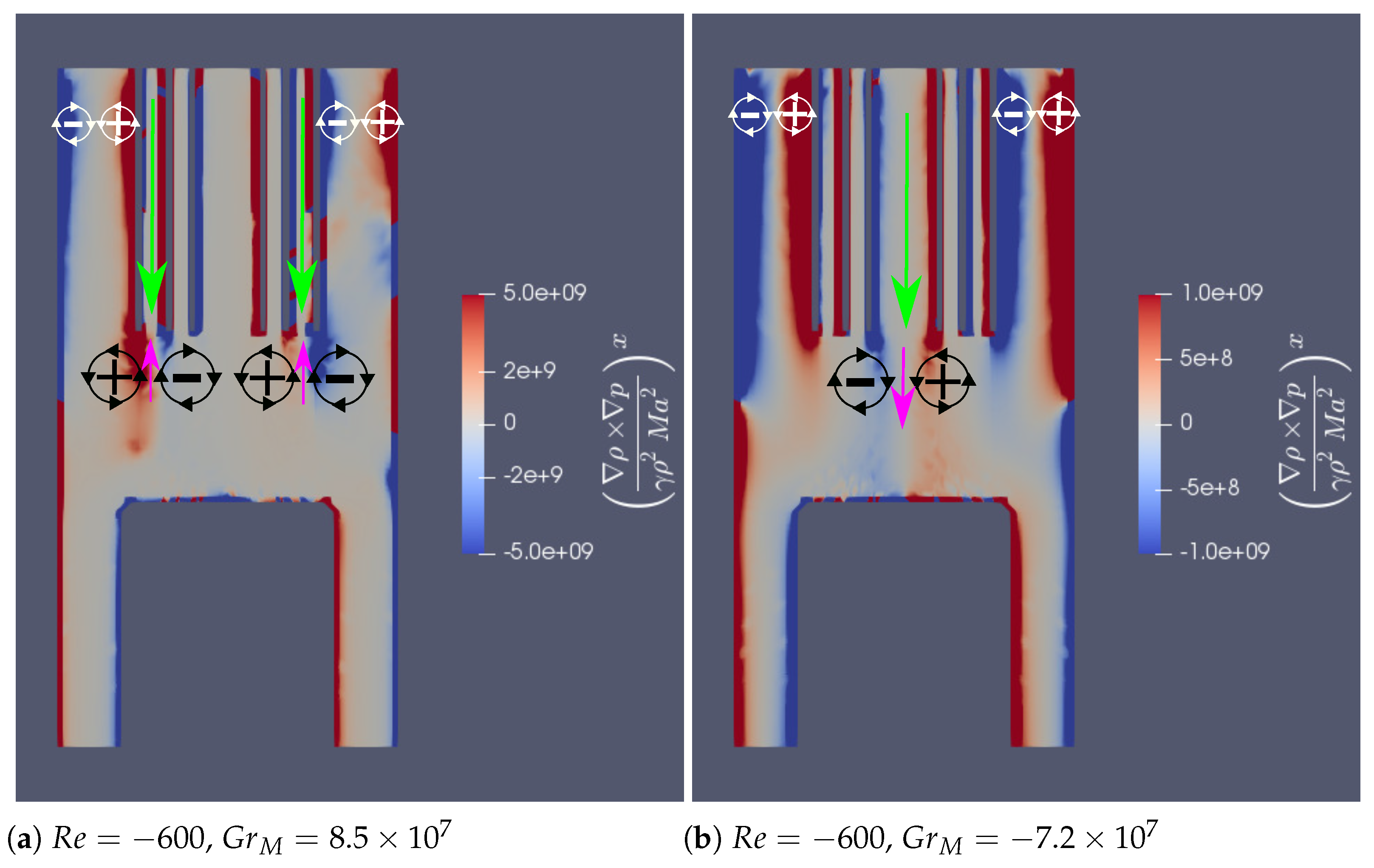
In case of the up-flow reactor, we again turn to the analysis of the effect of the baroclinic torque.
Figure 11 shows the distribution of the x-component of the baroclinicity in the up-flow reactor for the variation of NH
in the ORL (see
Figure 11a) and variation of
ratio in IRL (see
Figure 11b). In an analogy to the down-flow reactor, two regions of high baroclinicity can be identified, namely the outer walls and the area between the nozzle and the growth zone.
From
Figure 4 and
Figure 7 together with
Figure 5 and
Figure 8, we find that the instabilities in the outer part correlate with the
ratio rather than the
ratio and occur especially at high values of
, i.e., at small Re numbers. From
Figure 12, it can be concluded that these instabilities are again triggered by horizontal thermal gradients, as in the case of the down-flow reactor. However, one difference from the down-flow reactor is the small dependence of these instabilities on the
in the case of NH
in the ORL. Looking at the distribution of
in
Figure 3 and the baroclinic torque at the nozzle in
Figure 11, we find that the baroclinic torque becomes stronger with an increasing amount of NH
, pushing the gas flow towards the center. This results in a region with reduced fluid velocity at the outer wall in the mixing zone. This is also in line with the result from
Figure 5 that the region with instabilities extends with increasing
. Increasing the Re number will counteract this effect and suppress the instabilities in this part of the reactor.
Now, we focus on instabilities that occur in the inner part of the up-flow reactor. We investigate the results from the variation of GaCl and H
in the IRL first. From
Figure 11b, it can be seen that the baroclinic torque at the nozzle outlets caused by molar mass gradients is responsible for an acceleration of the fluid against its intended flow direction. This effect is accompanied by a transport of the gas away from the center of the reactor. This is underpinned by the results from
Figure 7 showing that these instabilities can be suppressed by decreasing
; see also
Figure 8b.
Now, we investigate the variation of NH
in the ORL; see
Figure 11a. In fact, the molar mass gradient between SWP and ORL is always positive, i.e.,
. However, the molar mass gradient between ORL and SL is always negative, i.e.,
. This results in a locally negative molar Grashof number, i.e.,
. Therefore, these instabilities follow the same root cause as in the case of the GaCl and H
in the IRL, namely, the acceleration of the fluid due to baroclinic torque induced by molar mass gradients is against its intended flow direction and therefore leads to instabilities. This is again underpinned by the results from
Figure 5b, where one finds that the condition of stability on the Reynolds number relaxes as
decreases.

 ,
, 


