Numerical Simulation of Species Segregation and 2D Distribution in the Floating Zone Silicon Crystals

Abstract

The distribution of dopants and impurities in silicon grown with the floating zone method determines the electrical resistivity and other important properties of the crystals. A crucial process that defines the transport of these species is the segregation at the crystallization interface. To investigate the influence of the melt flow on the effective segregation coefficient as well as on the global species transport and the resulting distribution in the grown crystal, we developed a new coupled numerical model. Our simulation results include the shape of phase boundaries, melt flow velocity and temperature, species distribution in the melt and, finally, the radial and axial distributions in the grown crystal. We concluded that the effective segregation coefficient is not constant during the growth process but rather increases for larger melt diameters due to less intensive melt mixing.

1. Introduction

The floating zone (FZ) method is used to produce silicon (Si) single crystals with high purity. In this method, a feed material is supplied as a polycrystalline rod, which is melted by a high-frequency inductor, and the molten Si flows along the open melting front (see the scheme in Figure 1). This forms a volume of melt, which cools and begins to crystallize at some distance from the inductor, thereby, creating the crystallization interface. The single crystal is then pulled downwards. Currently, needle-eye inductors (with the inner diameter smaller than the feed rod diameter) are used for the FZ process because they allow the use of a larger feed rod and achieve a larger crystal diameter.

To obtain the desired electrical resistivity of silicon crystals grown with the FZ method, it is necessary to precisely control the concentration of dopants—typically boron (B) or phosphorus (P) [1]. The level and distribution of various impurities, e.g., carbon (C), is also important in applications, such as the kilogram definition project [2]. A crucial phenomenon that defines the transport of such species is the segregation at the crystallization interface.

Let us consider a one-dimensional distribution of species concentration $C\left(z\right)$, where z is perpendicular to the crystallization interface, which is located at $z=0$; see Figure 2, left. The equilibrium segregation coefficient $k_0$ is theoretically defined as $\frac{C_s\left(0\right)}{C_m\left(0\right)}$, where $C_s\left(0\right)$ is the species concentration in solid silicon and $C_m\left(0\right)$ is in molten silicon at the interface.

However, crystal growth experiments with the same species (same $k_0$) can lead to different axial concentration distributions if other process parameters differ [3]. The effective segregation coefficient $k_{\mathrm{eff}}\equiv \frac{C_s\left(0\right)}{C_m(z\gg 0)}$ is more practical than $k_0$, because it considers the concentration outside the thin diffusion boundary layer $C_m(z\gg 0)$, which can be measured or evaluated more easily than $C_m\left(0\right)$. Therefore, $k_{\mathrm{eff}}$ also depends on the melt flow. An analytical expression for $k_{\mathrm{eff}}$ has been derived in the classical work by Burton, Prim and Slichter (BPS) [4]:

$$k_{\mathrm{eff}}=\frac{k_0}{k_0+(1-k_0)e^{-\frac{vd}{D}}},d\sim 1.6D^{\frac{1}{3}}{\eta }^{\frac{1}{6}}{\omega }^{-\frac{1}{2}},$$

(1)

where v is the crystallization velocity, d is the thickness of the diffusion layer in the melt, D is the diffusion coefficient of the impurity in the melt, $\eta$ is the kinematic viscosity, and $\omega$ is the crystal rotation rate. The shape of function $k_{\mathrm{eff}}\left(d\right)$ for three different species (carbon, phosphorus and boron) is shown in the right part of Figure 2. According to the BPS model, $k_{\mathrm{eff}}\ge k_0$, and, when the thickness of the diffusion layer increases (for example, due to a decrease in crystal rotation rate), $k_{\mathrm{eff}}$ increases and saturates at $k_{\mathrm{eff}}=1$ for large d. This saturation happens at smaller d for the species with a smaller diffusion coefficient.

Figure 2 shows that $k_{\mathrm{eff}}\left(d\right)$ can vary in a large interval, particularly for carbon. Moreover, the BPS model uses simplified assumptions of melt flow pattern and does not predict $k_{\mathrm{eff}}$ correctly in some cases (e.g., when melt flow is radially converging [5] or when microsegregation is taken into account [6]). Therefore, numerical flow simulations are necessary to obtain a more precise estimation of the effective segregation coefficient for FZ Si crystal growth.

Dopant segregation in the FZ process has been already studied in the literature—an axially symmetrical model of quasi-stationary dopant transport in the melt was described as early as 1997 [7]. Due to the increased availability of computational power, transient 3D simulations became possible around 2010 [8], and these kinds of simulations are still relevant now, e.g., for modelling radial resistivity distribution in 200 mm diameter FZ crystals [9]. However, all the aforementioned publications considered only the radial distribution of dopant concentration, without considering the axial distribution or the effective segregation coefficient.

The literature on $k_{\mathrm{eff}}$ of silicon impurities in crucible-free, inductively heated FZ processes was found to be scarce; therefore, we analyse other Si growth processes. An experiment has been reported that considered boron segregation during the Czochralski (CZ) process [10]. In that study, $k_{\mathrm{eff}}$ was found to be between 0.75 and 0.98, and it decreased when the melt flow became more intensive. This seemed to agree with the simplified BPS model (1): when the crystal rotation rate increased from 1 to 13 rpm, the diffusion layer became thinner, thus, diminishing $k_{\mathrm{eff}}$.

A study where the CZ crystal rotation was 16 rpm [11] reported a slightly smaller $k_{\mathrm{eff}}=0.73$. For crystals grown from a copper crucible using electron beam heating, $k_{\mathrm{eff}}$ was found to be 0.8 [12]. In yet another CZ experiment [13], boron $k_{\mathrm{eff}}$ approached 1 as the axial magnetic field increased. However, there are studies of oxygen transport in CZ Si that, on the contrary, indicate a lower $k_{\mathrm{eff}}$ when magnetic heaters are used [14]. The application of cusp magnetic field also lowered the oxygen content in grown crystals; however, it can be explained not only by the change in $k_{\mathrm{eff}}$—oxygen evaporation at the free surface may have played a large role [15].

In this study, we investigated the influence of the melt flow on $k_{\mathrm{eff}}$ in the Si FZ growth process and obtained the species distribution $C(r,z)$ in the entire grown crystal including the start cone and end cone growth stages, i.e., not only the radial profile $C\left(r\right)$ but also the axial profile $C\left(z\right)$. For the numerical simulations of the phase boundaries, electromagnetic field, melt flow, and species transport in the melt, we used previously developed numerical models.

The $k_{\mathrm{eff}}$ was then evaluated from the species concentration distribution in the melt. We created a new program that calculates the evolution of the average species concentration in the melt over time, which influences the species distribution along the crystal axis. To cover a wide range of $k_0$, we simulated two species: carbon ($k_0=0.07$) and boron ($k_0=0.8$).

2. Numerical Model

The present section describes the system of numerical models used for the modelling of the FZ crystal growth process. For the previously published models, only a brief summary and references are given in the following subsections.

This system of models is used to describe the following aspects of the FZ process: the shape of phase boundaries, electromagnetic (EM) field, melt flow, species transport in the melt and, finally, species distribution in the grown crystal. Section 2.1 presents a graphical and textual overview of the used models and data. The section explains how the simulated phase boundaries and EM field are used for the 3D melt flow simulations.

The melt flow simulations, in turn, are necessary for obtaining the effective segregation coefficient $k_{\mathrm{eff}}$. When $k_{\mathrm{eff}}$ is known, we can simulate the evolution of the average species concentration in the melt, which translates to the axial species distribution in the grown crystal. Section 2.2, Section 2.3 and Section 2.4 then focus on three main parts of the system of models: the phase boundaries, melt flow and species distribution in the crystal.

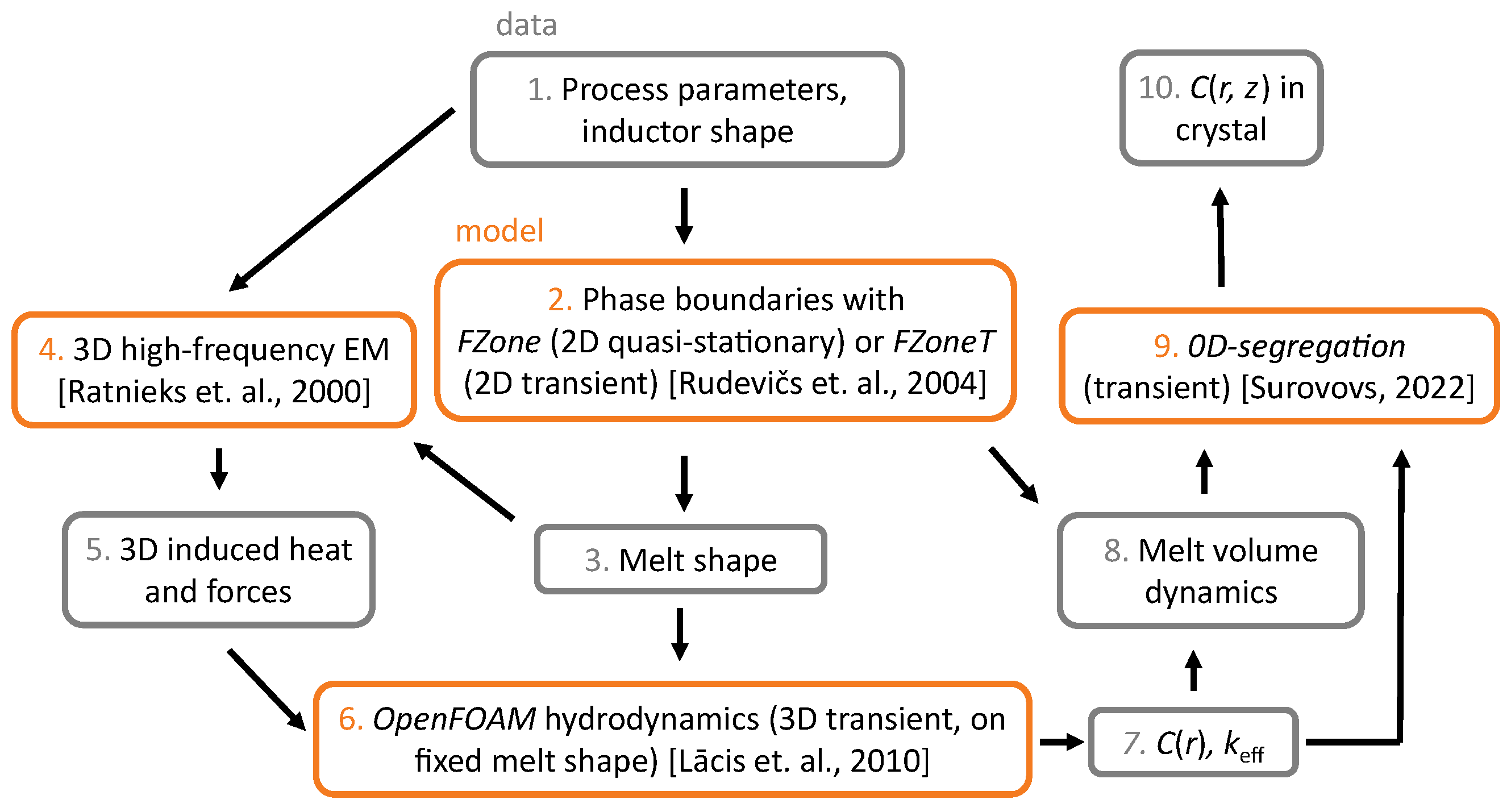
2.1. Overview of Modelling Scheme

The overall scheme of the models and their interactions is shown in Figure 3. The used data (or the obtained results) are shown in grey boxes, while the models are shown in orange boxes. In the beginning, one needs to specify the process parameters (see grey box No. 1): the zone height, inductor frequency, system geometry, etc. For the modelling of phase boundaries (orange box 2), one of two programs can be used: a quasi-stationary program FZone [16], which is suitable only for the cylindrical phase, or a transient program FZoneT [17], which describes the entire process: start cone, cylinder and end cone.

Both programs assume the axially symmetrical (also denoted by 2D) approximation of the shape of silicon parts. FZone and FZoneT programs are used to calculate melt shape (box 3). FZoneT also allows obtaining the melt volume dynamics (box 8): the history of the change in crystal diameter, melt volume, etc. More information about these programs is given in Section 2.2.

Using the obtained melt shape, a 3D finite volume mesh is created for OpenFOAM [18] hydrodynamic simulation (box 6). This includes transient simulation of the melt flow, heat transfer and species transport; see Section 2.3. To obtain boundary conditions for the melt velocity and temperature at the free surface, a 3D inductor shape is used to calculate the induced heat and Lorentz forces [19] (boxes 4 and 5).

OpenFOAM hydrodynamic simulation produces the radial distribution of the species concentration $C\left(r\right)$ in the grown crystal and the effective segregation coefficient $k_{\mathrm{eff}}$. This data, together with the melt volume dynamics, is then used in the transient 0D-segregation program (box 9), which predicts the temporal evolution of the average species concentration in the melt [20]. The complete description of the mathematical model for 0D-segregation is presented in Section 2.4. Finally, the results of 0D-segregation program are interpolated on the point grid that is created in crystal domain (box 10); this process is schematically shown in Figure 4.

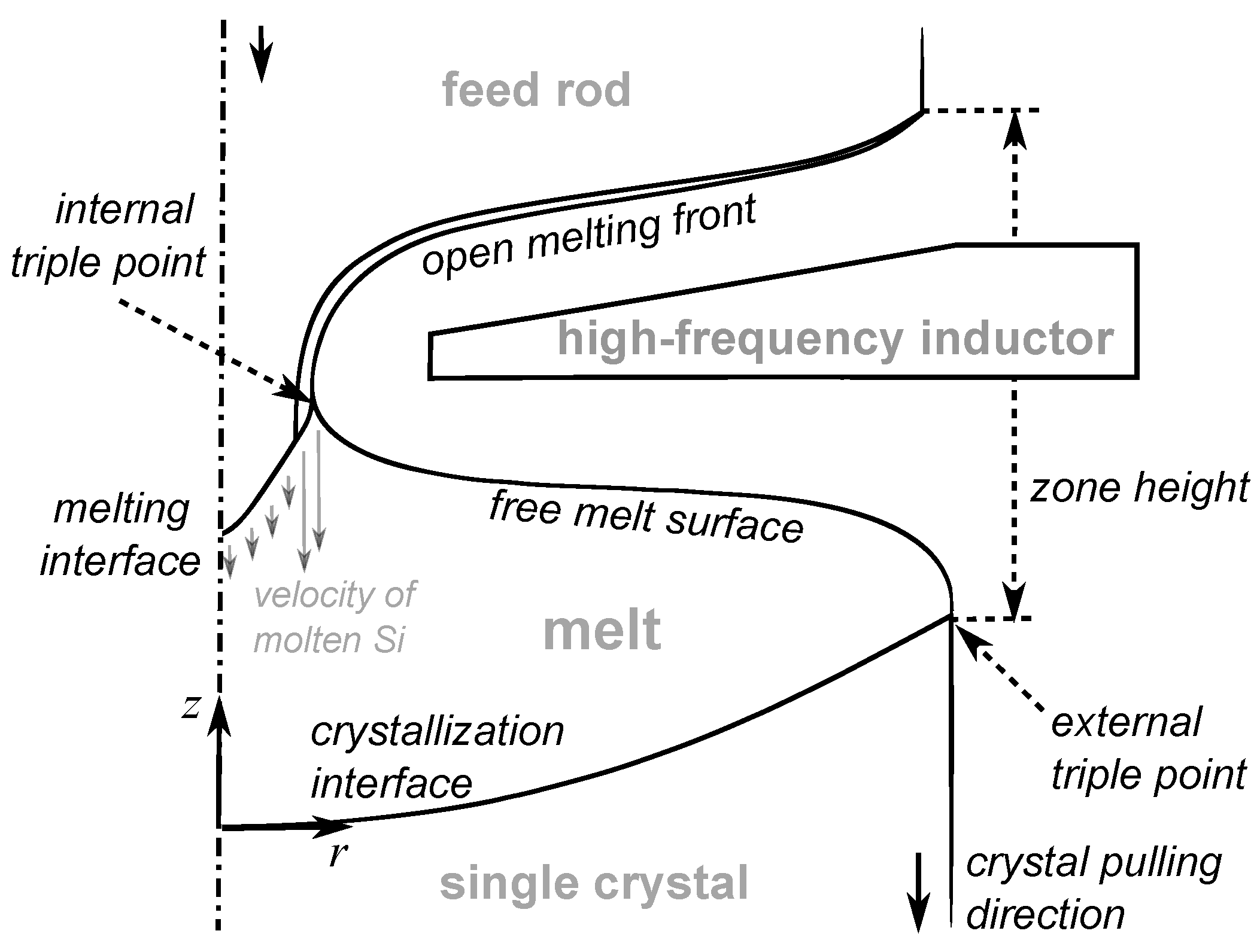
2.2. Phase Boundaries

The description of the program FZone, which has been used for the calculation of phase boundaries, is provided in [16]. The program considers axially symmetrical approximations of phase boundaries. The melting interface, crystallization interface and open melting front are moved according to the heat flux balance; the influence of the melt flow is neglected. The program FZone operates in quasi-stationary approximation: it describes the cylindrical phase of the process, i.e., it calculates the shape of the phase boundaries for a process stage when they do not change in time.

The transient version of this program that simulates growth process dynamics (e.g., a change in the crystal radius during the cone phase) is called FZoneT  [17]. The evolution of the crystal diameter and melt volume is saved in a file, which can be later read by the 0D-segregation program. The species concentration inflow from the melting feed rod (the integral from Equation (3)) is also saved in a file. In the present work, the transient FZoneT program was used to simulate the entire crystal growth (the start cone, cylinder and end cone), and the results from three time instants from the start cone stage were selected for melt flow simulations.

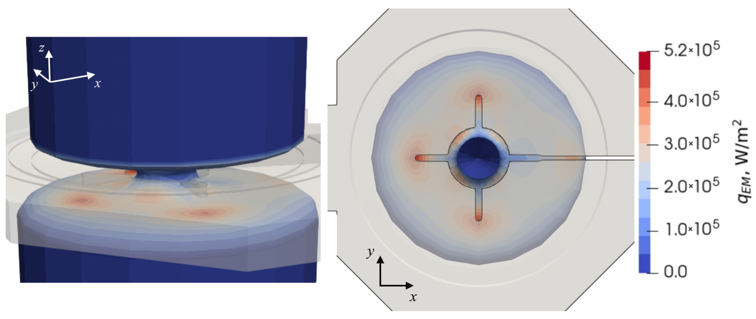
2.2.1. Electromagnetic Field

When quasi-stationary FZone is used, the EM field is calculated in 3D using boundary elements and assuming negligible skin depth [19]. The EM field is iteratively recalculated until the shape of the phase boundaries converges. However, in the transient FZoneT version, only an axially symmetrical (also denoted by 2D) EM field is simulated due to limited computational resources. In the 2D EM simulations, inductor slits are modelled by setting an artificial magnetic field source surface density [16], which allows part of the magnetic field lines to penetrate the inner part of the inductor.

To calculate the 2D EM field distribution, axially symmetrical inductor shape was constructed in a way that ensures the best correspondence to the results obtained with a 3D non-symmetrical shape. Quasi-stationary simulations of the corresponding 3D system were performed to calibrate 2D inductor characteristics so that the differences between the induced power on the silicon surface are the smallest (the results are presented in Section 3.2.2). A similar comparison of different EM field models is described in [21].

The initial simulations were performed using real slit parameters in the 2D model. Then, the width and length of the inductor side slits as well as the width of the main slit were changed to achieve better agreement between 2D and 3D systems.

2.3. Species Transport in Melt

The species transport in melt is simulated with the OpenFOAM hydrodynamic solver described in [22]. This assumes fixed phase boundaries and uses the transient, incompressible, laminar Navier–Stokes equation for melt velocity, with the Boussinesq approximation for the description of thermal convection. Boundary conditions for velocity are as follows:

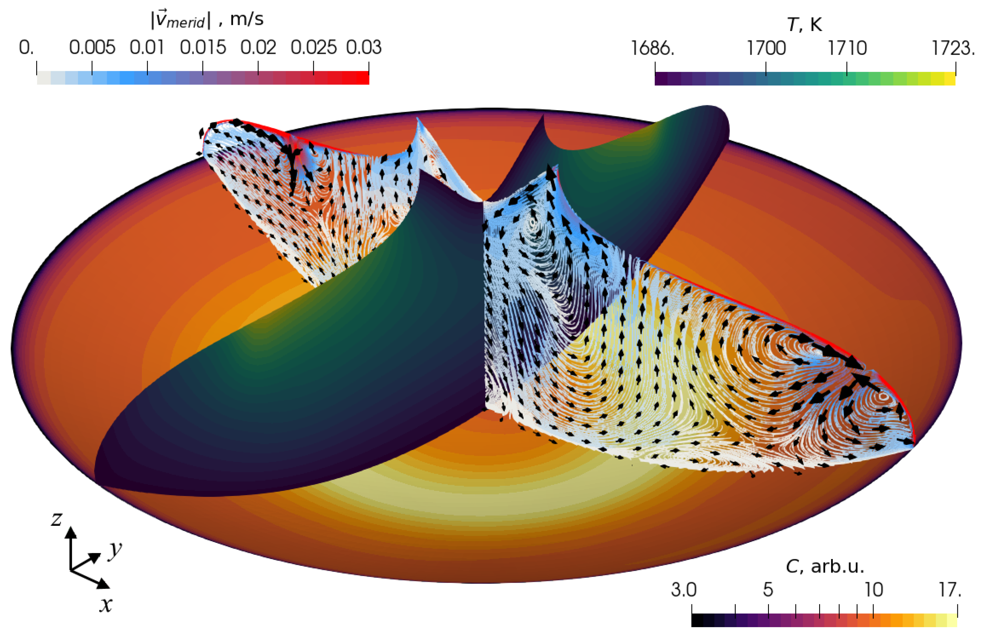
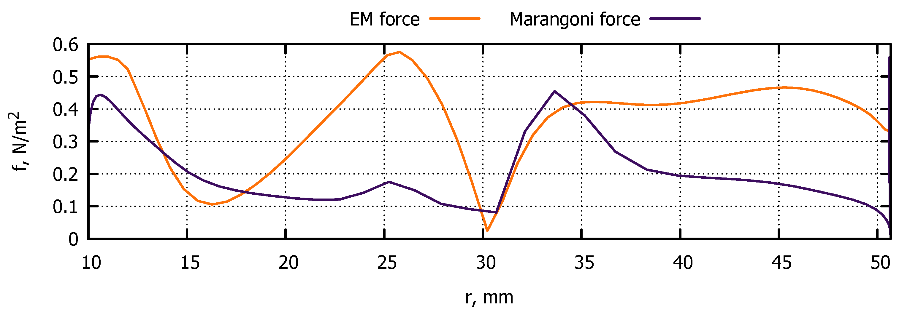
• Marangoni force and the EM force are applied on the free melt surface.
• Fixed velocity (crystal pulling speed and rotation)—on the crystallization interface.
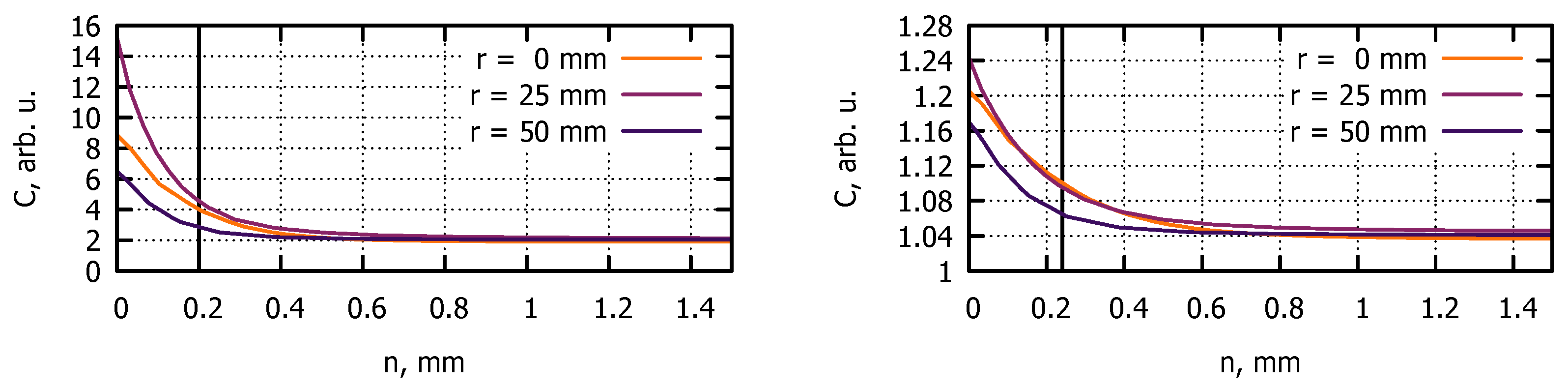
• Fixed velocity (feed rod pushing speed and ring-shaped inflow from the open melting front; see Figure 1)—on the melting interface [18,23].

A standard convection-diffusion equation is used for simulation of the melt temperature with the EM-induced heat and radiation on the free melt surface and fixed temperature on the solid–liquid interfaces. The equation that describes species transport is also of the convection-diffusion type:

$$\frac{\partial C}{\partial t}+(\overrightarrow{v}\nabla )C=D\mathrm{\Delta }C,$$

(2)

where C is the species concentration, t is the time, $\overrightarrow{v}$ is the melt velocity, and D is the species diffusion coefficient. The initial conditions were uniform: $C=1$ arb.u. (arbitrary unit). The boundary conditions for concentration are as follows:

• On the crystallization interface: $D\frac{\partial C}{\partial n}=v_C(1-k_0)Ccos\theta ,$ where n is the normal coordinate, $k_0$ is the segregation coefficient, and $\theta$ is the the angle between the horizontal plane and the interface normal vector.
• On the melt free surface: $\frac{\partial C}{\partial n}=0$ due to the assumption of a pure gas atmosphere and lack of evaporation [24].
• On the melting interface: $C=1$ arb.u., i.e., the species concentration is normalized to the initial concentration in the feed rod, which is assumed to be homogeneous.

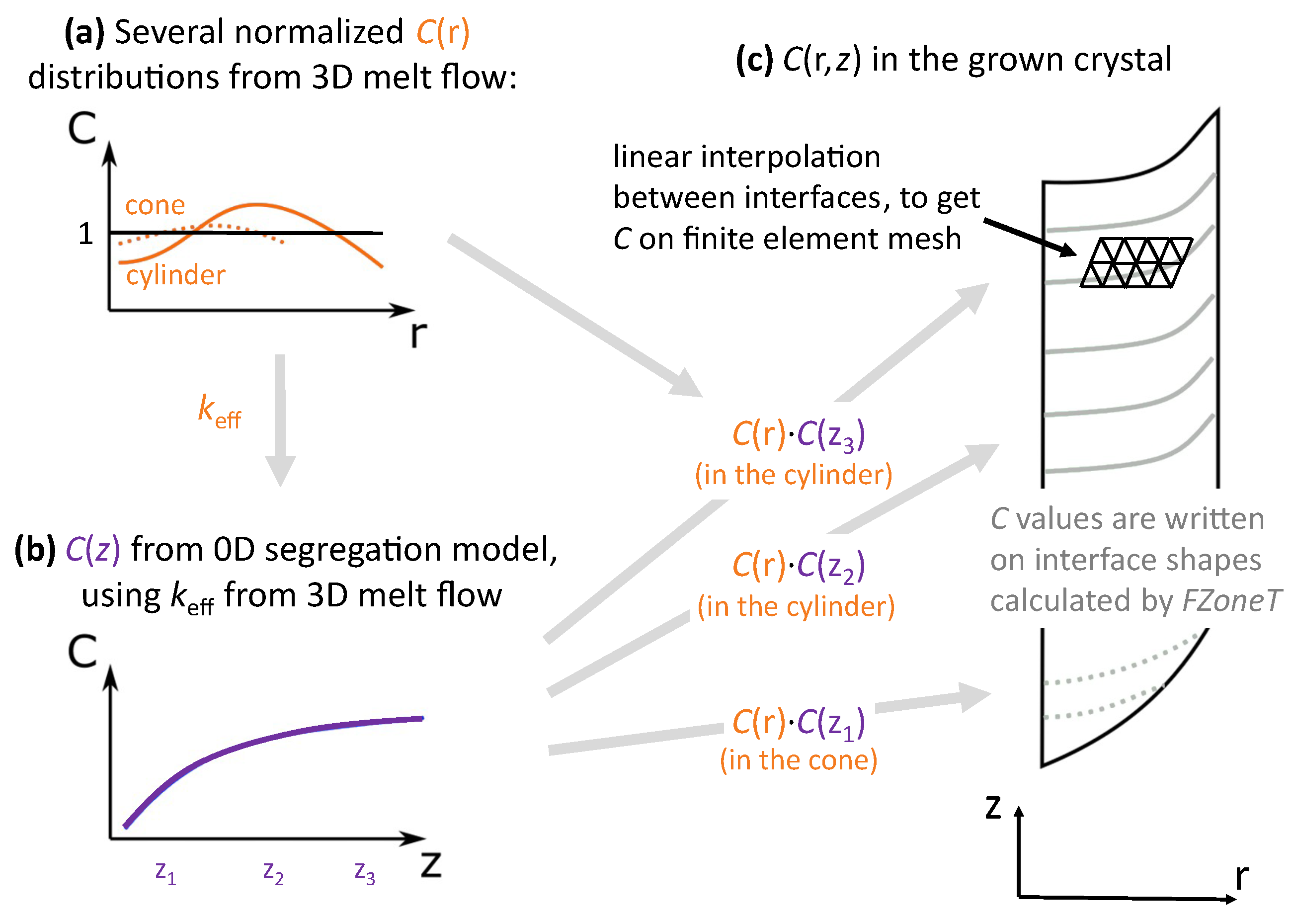
2.4. 2D Species Distribution in Crystal

To simulate the axial distribution of species in the crystal, the time-dependence of the average species concentration in the melt $C_m\left(t\right)$ was considered. It was assumed (and later supported by simulation results; see Section 3.3.1) that the $\overrightarrow{v}$ and $C_m$ in the melt reach a quasi-stationary state sufficiently fast in comparison to the characteristic time of axial changes of concentration in the grown crystal. Therefore, we assumed that the average concentration of species in the crystallizing silicon at any given time t is directly proportional to $C_m\left(t\right)$. Thus, the following equation of species mass conservation was proposed:

$$\mathrm{\Delta }\left(C_m{V}_m\right)=\int C_F{v}_F\mathrm{\Delta }t\mathrm{d}S-k_{\mathrm{eff}}{C}_m\mathrm{\Delta }{V}_{\mathrm{out}},$$

(3)

where $V_m$ is the melt volume, $C_F$ is the species concentration in the feed rod at the melting interface, $v_F$ is the feed rod pushing rate, $\mathrm{\Delta }t$ is the simulation time step, $\mathrm{d}S$ is the surface element of melting interface and open melting front, $k_{\mathrm{eff}}=C_C/C_m$ is the effective segregation coefficient, $\mathrm{\Delta }{V}_{\mathrm{out}}$ is the volume of the crystal that crystallizes during the time step, and $C_C$ is the average species concentration in the layer that crystallizes during the time step. The value of $k_{\mathrm{eff}}$ is obtained from OpenFOAM simulations (see Section 3.3.1) and can depend on the process parameters, e.g., the crystal diameter $D_C$.

Equation (3) can be rearranged to express $\mathrm{\Delta }{C}_m$, which then is used to calculate $C_m$ iteratively with the time step $\mathrm{\Delta }t$:

$$\mathrm{\Delta }{C}_m{V}_m=-C_m\mathrm{\Delta }{V}_m+\int C_F{v}_F\mathrm{\Delta }t\mathrm{d}S-k_{\mathrm{eff}}{C}_m\mathrm{\Delta }{V}_{\mathrm{out}},$$

$$\mathrm{\Delta }{V}_{\mathrm{in}}=\int v_F\mathrm{\Delta }t\mathrm{d}S$$

$$\mathrm{\Delta }{V}_m=\mathrm{\Delta }{V}_{\mathrm{in}}-\mathrm{\Delta }{V}_{\mathrm{out}}$$

$$C_m(t+\mathrm{\Delta }t)=C_m+\mathrm{\Delta }{C}_m=C_m+\frac{C_m(\mathrm{\Delta }{V}_{\mathrm{out}}-\mathrm{\Delta }{V}_{\mathrm{in}})+\int C_F{v}_F\mathrm{\Delta }t\mathrm{d}S-k_{\mathrm{eff}}{C}_m\mathrm{\Delta }{V}_{\mathrm{out}}}{V_m}.$$

(4)

Equation (4) is implemented using Python language. This program is called 0D-segregation, because it describes transient species segregation without spatial dimensions, i.e., disregarding spatial concentration distribution in the melt. The program source code is published in [20]. Two functionalities of the program are available:

• Importing the data about process dynamics (time-dependent $V_m$, $C_F$, $\mathrm{\Delta }{V}_{\mathrm{out}}$ and $\mathrm{\Delta }{V}_{\mathrm{in}}$) from transient phase boundary simulations with FZoneT.
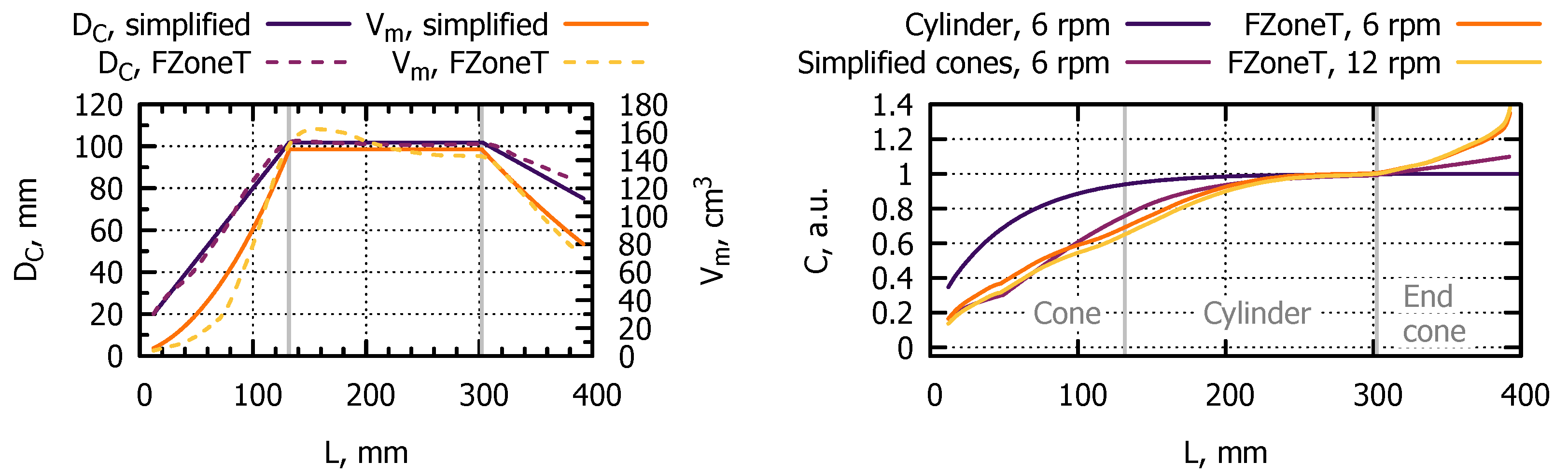
• Creating an approximate description of the cone phase based only on the simplified crystal shape described as $D_C\left(L\right)$, where L is the crystal length:
  • Due to the assumption of constant pulling velocity, $L\propto t$.
  • Cone surfaces are approximated as having constant slope, and thus $D_C\left(t\right)\propto t$.
  • The free surface height above the external triple point is assumed to be constant even during the cone phases because it is impossible to predict its evolution for an arbitrary crystal shape (without experimental data); therefore, $V_m\left(t\right)\propto D_C{\left(t\right)}^2$.
  • The crystallized volume is proportional to the crystal cross-section: $\mathrm{\Delta }{V}_{\mathrm{out}}=v_C{S}_C\mathrm{\Delta }t$, where $v_C$ is the crystal pulling velocity, and $S_C=\frac{\pi }{4}{D}_C{\left(t\right)}^2$ is the crystal cross-section area. Therefore, $\mathrm{\Delta }{V}_{\mathrm{out}}\propto D_C{\left(t\right)}^2$.
  • Due to silicon mass conservation, $\mathrm{\Delta }{V}_{\mathrm{in}}=\mathrm{\Delta }{V}_m+\mathrm{\Delta }{V}_{\mathrm{out}}$.

After $C_m\left(t\right)$ has been calculated, it is combined with $C\left(r\right)$, which was obtained during species transport simulations in melt; see the scheme in Figure 4. The final result is $C(r,z)$ distribution in the grown crystal.

3. Results

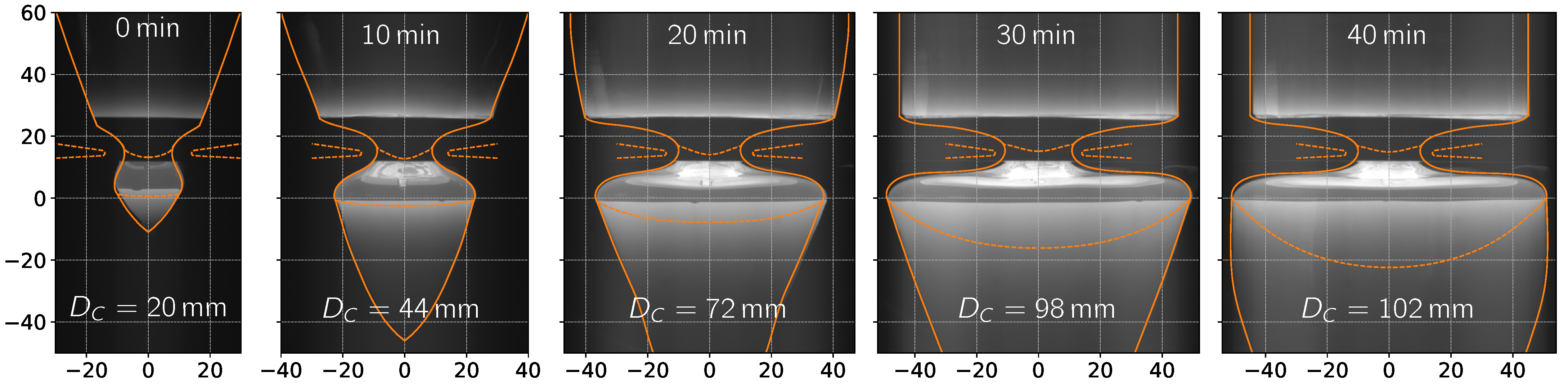
3.1. Description of the Experiment

The present work uses process data from a 4″ FZ crystal growth experiment performed at the IKZ (Leibniz Institute for Crystal Growth, Berlin). The main parameters are listed in

Table 1. Parameters of the experiment.

Parameter	Value
Crystal diameter $D_C$	102 mm (cylinder phase)
Feed rod diameter $D_F$	90 mm
Crystal pulling rate $v_C$	3.5 mm/min
Feed rod push rate $v_F$	4.5 mm/min (cylinder phase)
Crystal rotation rate ${\omega }_C$	6 rpm
Feed rod rotation rate ${\omega }_F$	−0.8 rpm
Zone height $H_Z$	27 mm (cylinder phase)
Inductor frequency f	3 MHz

. A standard one-turn inductor with three side slits is used; see Figure 5 and our earlier work [25,26]. The shape of the grown crystal as well as the height of the molten zone can be seen in Section 3.2.3, where a comparison to transient simulation results is performed. Process photographs with the visible parts of the phase boundaries were used to validate the simulation of the cone phase in particular. Note that characterization of the grown crystals is not discussed in the present study and will be addressed in further publications.

3.2. Phase Boundaries

3.2.1. Quasi-Stationary Simulations

First, quasi-stationary simulations are performed with FZone program to obtain the shape of phase boundaries for the system described in Section 3.1, which are later used in hydrodynamics simulations in Section 3.3. 3D EM simulations are performed to precisely describe the EM field created by the high-frequency inductor. An example of the results of 3D EM simulations (induced heat on silicon free surface) is shown in Figure 5.

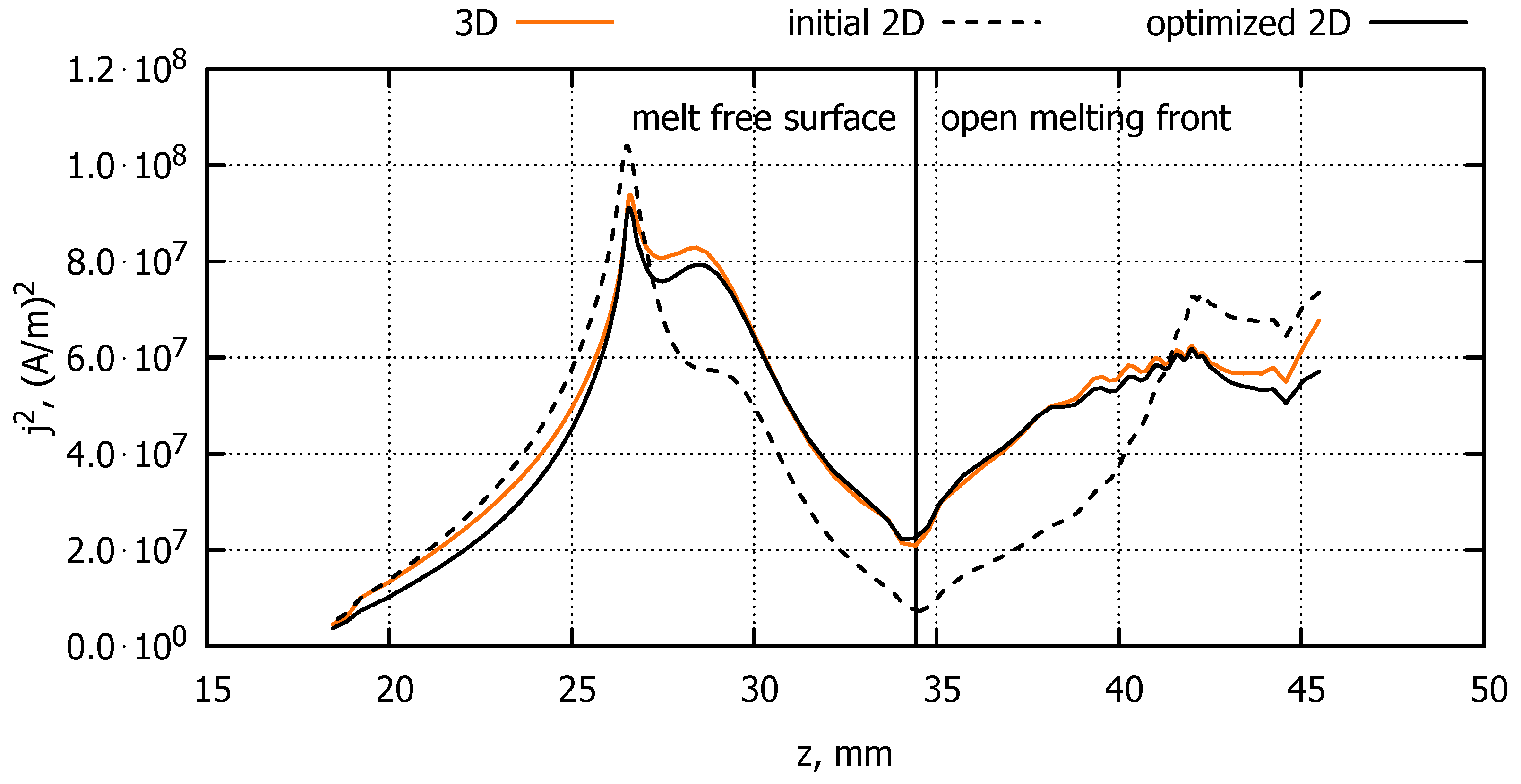
3.2.2. Influence of Three-Dimensionality of the EM Field

Three-dimensional melt flow simulations require 3D distributions of induced heat and Lorentz force, which can only be achieved using a 3D model of the high-frequency inductor shape. On the other hand, transient simulations can be performed only with a 2D EM field model, which approximates the 3D features of the asymmetrical EM field (see Section 2.2.1).

Induced current on the open melting front and the free melt surface of silicon are compared between different EM models in Figure 6. For the 3D model, the azimuthally averaged radial distribution is shown. In the case of the 2D model, the effect of inductor slits can be considered only approximately, which results in a significantly different distribution. Various parameter studies were conducted to obtain the optimal inductor parameters (modified slit width and length).

The resulting induced electrical current distribution from the optimized 2D model is similar to the 3D model results with the same defined inductor current. The main differences can be observed on the free melt surface and in the outer part of the open melting front. This results in slightly different shapes of the phase boundaries, which are shown in Figure 7. The internal triple point radius is slightly smaller, which results in a different melting interface and free melt surface shape. However, the 2D model is sufficiently precise to describe the melt volume dynamics, because the differences are large only in the central part of the melt.

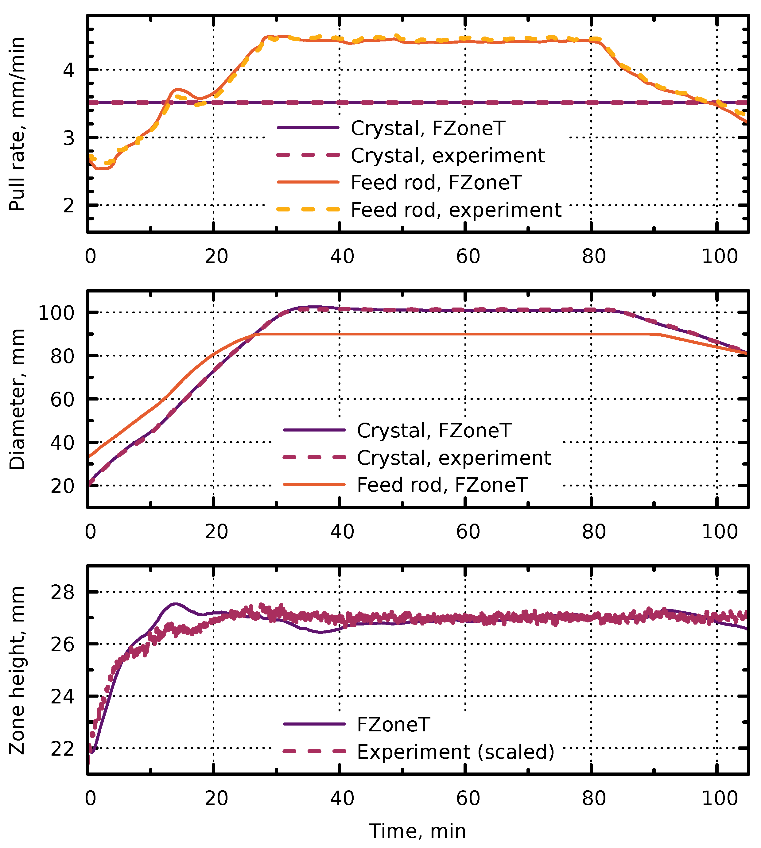
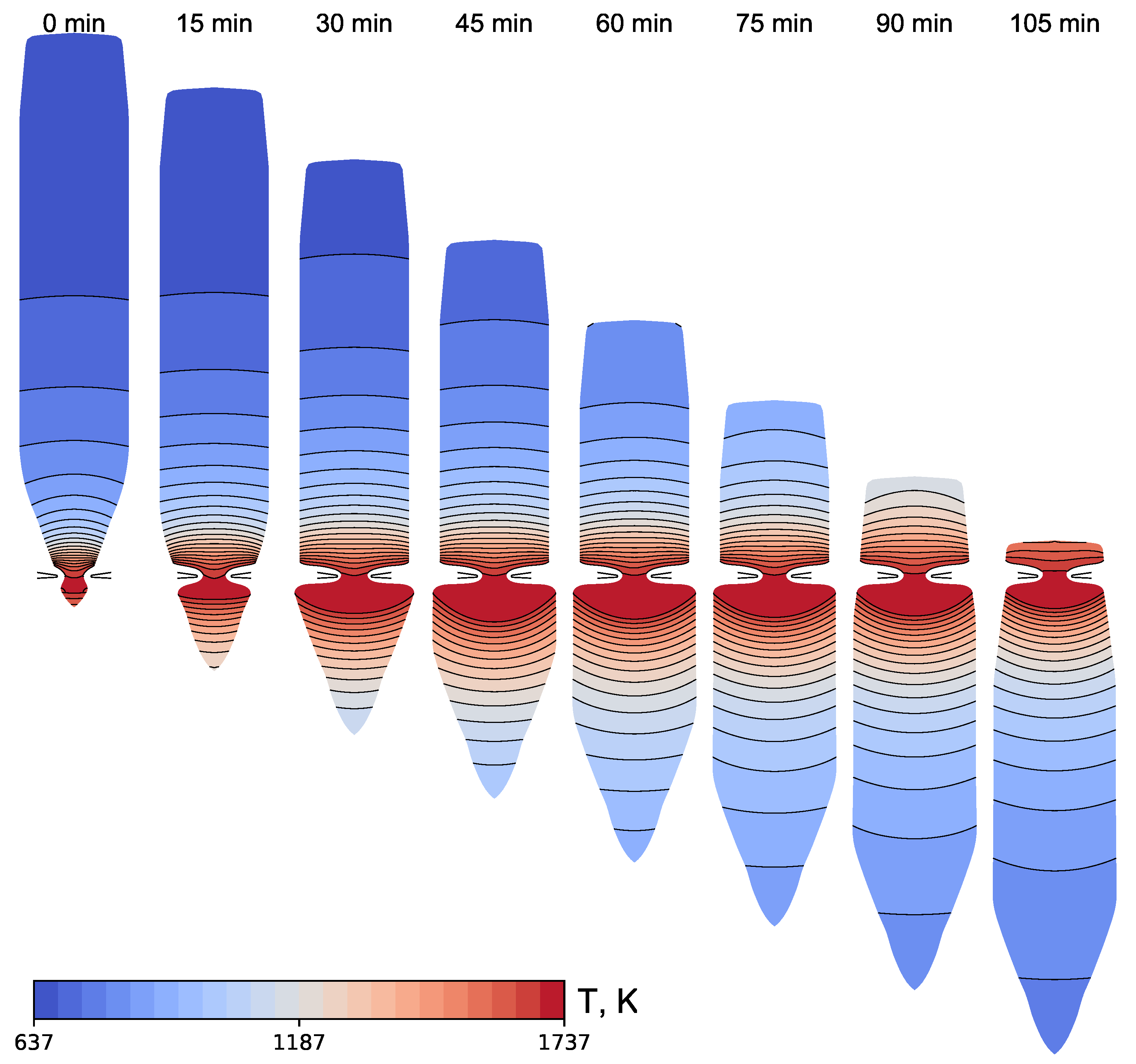
3.2.3. Transient Simulations

While the quasi-stationary approach used in FZone was applied in the present work for the cylindrical growth stage, the transient model should be considered for the initial and final stages of the process when the crystal or feed rod is short and the diameter is changing. Therefore, a transient simulation of the temperature field and phase boundaries has been conducted using FZoneT, starting from a small cone with a diameter of 20 mm and a length of 12 mm at time $t=0\mathrm{m}\mathrm{i}\mathrm{n}$. A rather good agreement with the experiment was obtained for the shape of the phase boundaries during the cone and cylindrical growth stages; see Figure 8.

The time-dependent inductor current (instead of the power used in the experiment) and feed rod velocity were adjusted to achieve good agreement with the experimentally measured crystal diameter and zone height as demonstrated in Figure 9. A slightly imperfect prediction of the zone height by FZoneT could be caused by differences in input data (inductor current and feed velocity) or by model limitations (e.g., a fluid film model describing the melting of a macroscopically smooth open melting front).

The feed diameter $D_F$ was not explicitly measured in the experiment; therefore, only the curve from FZoneT is plotted in Figure 9. It was verified that $D_F$ during the cylindrical growth stage was 90 mm both in the experiment (from process photos) and FZoneT simulation in accordance with the steady-state mass conservation $D_F=D_C\sqrt{v_C/v_F}$.

An example of the calculated global temperature field and shape of phase boundaries during the entire process is shown in Figure A1 of Appendix A.

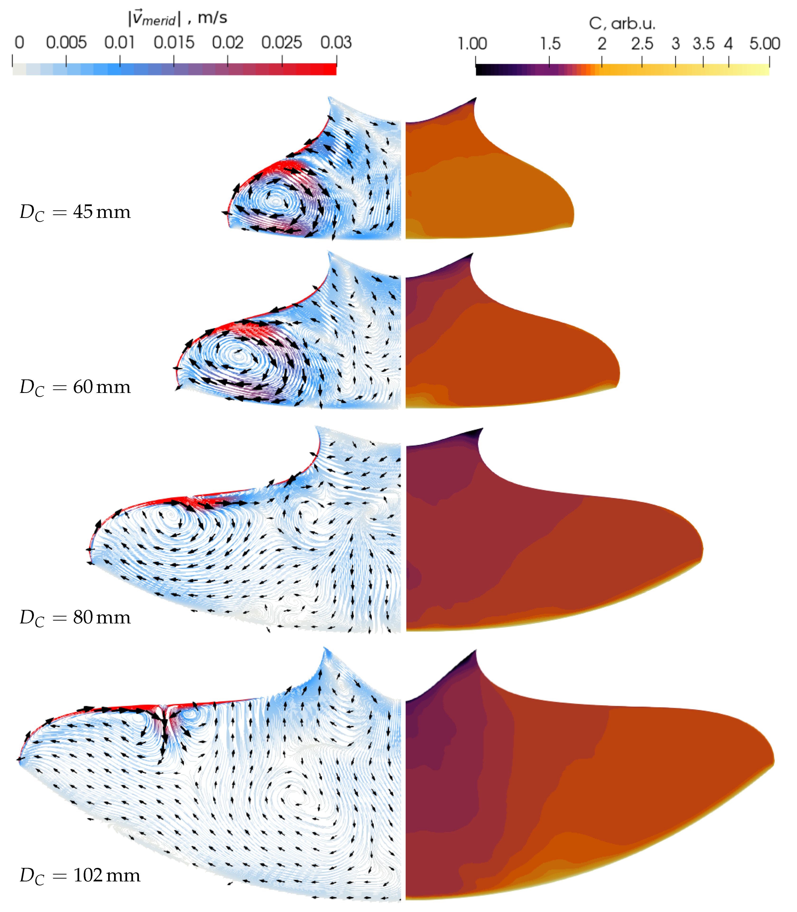
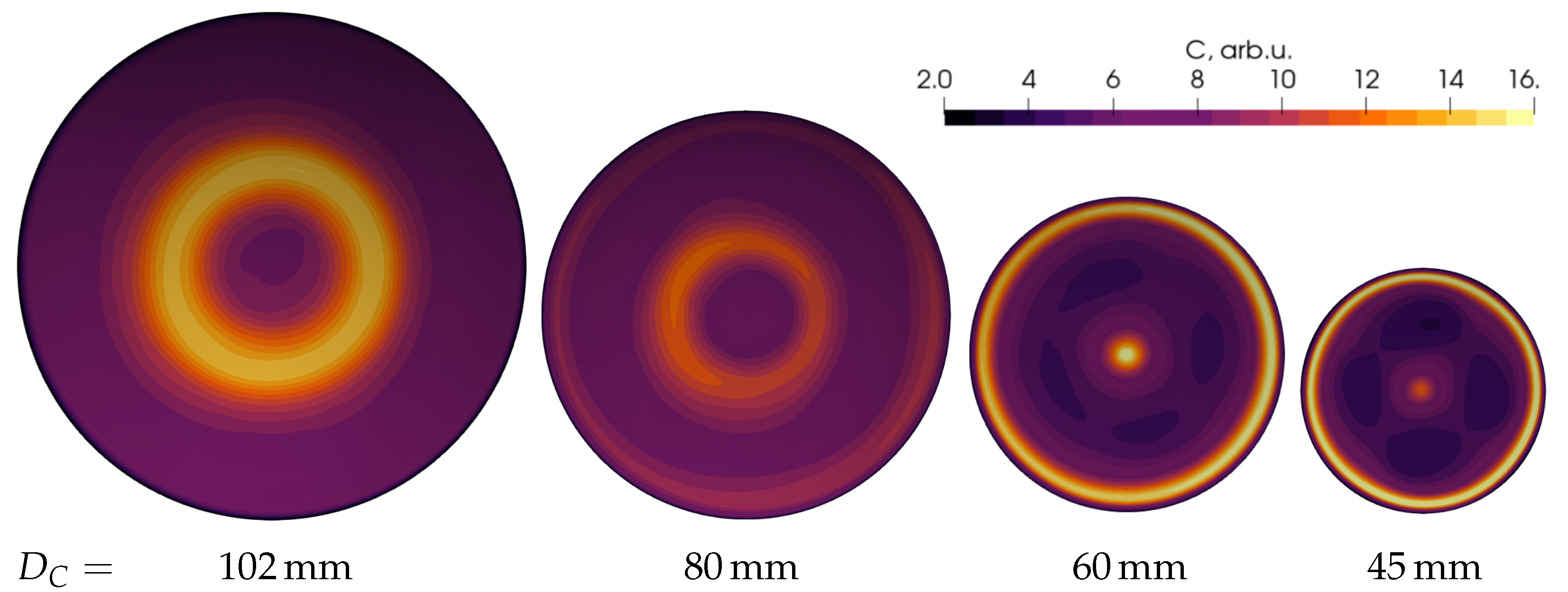
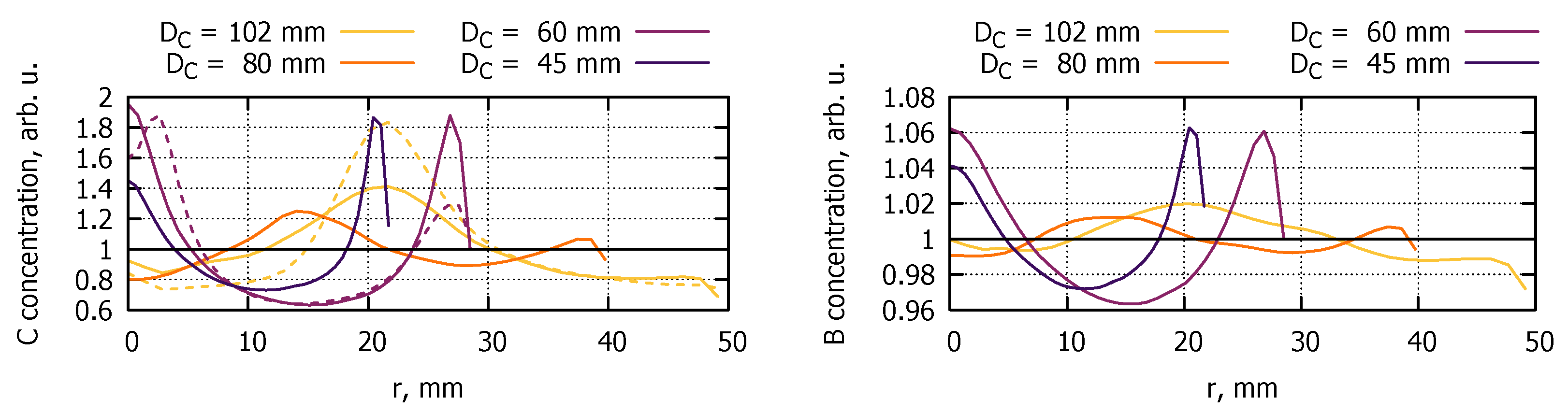
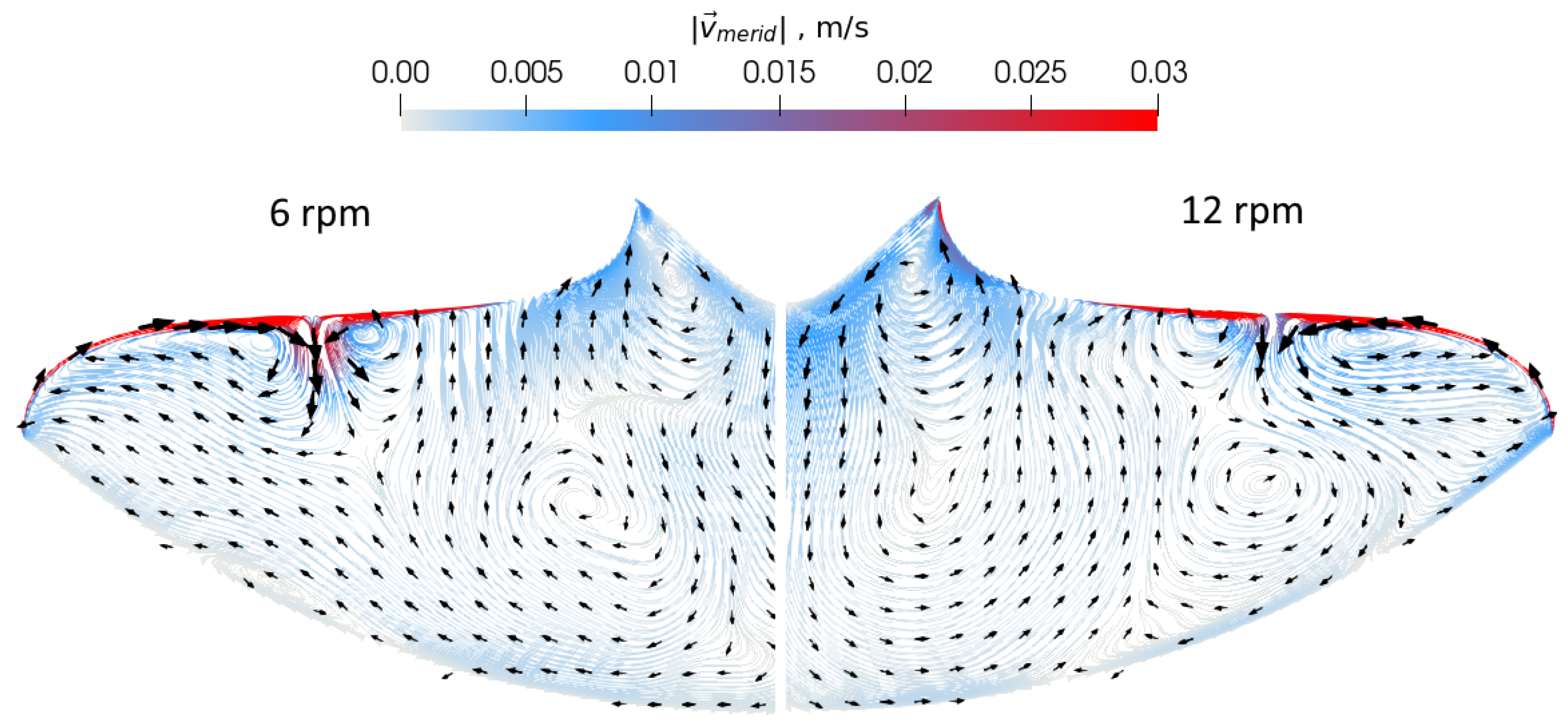
3.3. Species Transport in Melt

Using the simulated phase boundaries, that were obtained using FZone or FZoneT and presented in the previous section, 3D melt flow simulations were run with OpenFOAM using the model described in Section 2.3. The most important physical and numerical parameters are given in

Table 2. The physical [27] and numerical parameters that were used for OpenFOAM simulations.

Parameter	Value
Silicon density $\rho$	$2580\mathrm{k}\mathrm{g}/{\mathrm{m}}^3$
Silicon viscosity $\eta$	$8.6·{10}^{-4}\mathrm{P}\mathrm{a}·\mathrm{s}$
Silicon heat conductivity $\lambda$	$67\mathrm{W}/\mathrm{m}·\mathrm{K}$
Silicon specific heat capacity $c_p$	$1000\mathrm{J}/\mathrm{k}\mathrm{g}·\mathrm{K}$
Silicon thermal expansion coefficient $\beta$	${10}^{-4}1/\mathrm{K}$
Marangoni coefficient M	$-1.3·{10}^{-4}\mathrm{N}/\mathrm{m}·\mathrm{K}$ [26]
Carbon diffusion coefficient D	$7·{10}^{-9}{\mathrm{m}}^2/\mathrm{s}$ [28]
Carbon segregation coefficient $k_0$	0.07 [3]
Boron diffusion coefficient $D^{\prime }$	$1.2·{10}^{-8}{\mathrm{m}}^2/\mathrm{s}$ [29]
Boron segregation coefficient $k_0^{\prime }$	0.8 [29]
Total number of mesh elements	614,000
Largest element size	0.8–1.4 mm (inside the melt)
Smallest element thickness	0.02–0.03 mm (at the crystallization interface)
Time step	2 ms
Total simulation time	350–500 s
Averaging interval for $C,T,\overrightarrow{v}$	100 s

. An example of the simulation results for the carbon transport during the cylindrical phase is shown in Figure 10. Despite the non-symmetrical high-frequency inductor, the carbon concentration field is mostly axially symmetrical.

The OpenFOAM simulations can be performed only using a fixed melt shape (stationary phase boundaries). The FZone calculation of the cylindrical growth stage with a diameter of 102 mm was used. In addition, the results from FZoneT with several cone diameters were selected to simulate the melt flow in a cone phase: 80, 60 and 45 mm.

The simulated melt velocity in the vertical plane parallel to the main inductor slit is shown in Figure 11, left. Comparison between the EM and Marangoni force densities on the free surface shows that the EM forces dominate; see Figure 12. The EM force is creating an inwards-directed flow at the outer part of the melt. The melt flow is more intensive for the smaller $D_C$ due to larger EM field gradients.

The flow pattern is similar between two stages with larger $D_C$, where the largest velocities (exceeding 1 cm/s) appear only near the free surface and in the neck region.

The decrease in the melt flow intensity during the increase in $D_C$ may be related to various factors. One of them could be the EM force redistribution due to the change in the free surface shape. The influence of crystal rotation on larger melts could also play a role: when the azimuthal melt velocity is higher, it is more difficult to induce a radial flow [7]. Another possible explanation is different surface-to-volume ratios, which decrease the influence of the surface EM force for larger $D_C$.

The carbon concentration distribution is shown in Figure 11, right. Arbitrary units are used, and normalization is made with respect to the concentration in the feed rod, i.e., the $C=1$ boundary condition is set on the melting interface. Concentration contours, despite the averaging over 100 s, are not always smooth—possibly due to the chaotic temporal behaviour of the melt flow or due to minor numerical effects, e.g., mesh non-orthogonality.

As of segregation with small $k_0$, a thin boundary layer is formed at the crystallization interface; see Figure 13. The width of this layer approximately corresponds to the values calculated using the BPS model, Equation (1): 0.020 mm for carbon and 0.024 mm for boron. The carbon concentration at the crystallization interface is shown in Figure 14. The obtained concentration distributions for large $D_C$ are axially symmetrical due to crystal rotation and due to partial axial symmetry of the boundary conditions.

For smaller $D_C$, only minor deviations from the axial symmetry in the concentration distribution are present, and they do not significantly affect the azimuthally averaged radial distribution. There is no experimental data about such 2D distributions known to the authors.

From the species concentration values at the interface, as shown in Figure 14, the radial distribution of species atoms in the grown crystal can be calculated; see Figure 15. For small $D_C$ (60 mm and less), two distinct concentration maxima exist: one in the crystal centre and one near the rim. This effect can be explained by the intensive melt vortex, as shown in the top images in Figure 11. Such a central maximum of species concentration in small crystals ($D_C=40\mathrm{m}\mathrm{m}$) was also observed in experiments [30]. When $D_C$ is large ($D_C=102\mathrm{m}\mathrm{m}$), the species concentration maximum is obtained at $r\approx 20$ mm. It corresponds well to the resistivity maximum that is obtained due to the distribution of phosphorus or other dopant elements in typical $4^{″}$ silicon crystals [31].

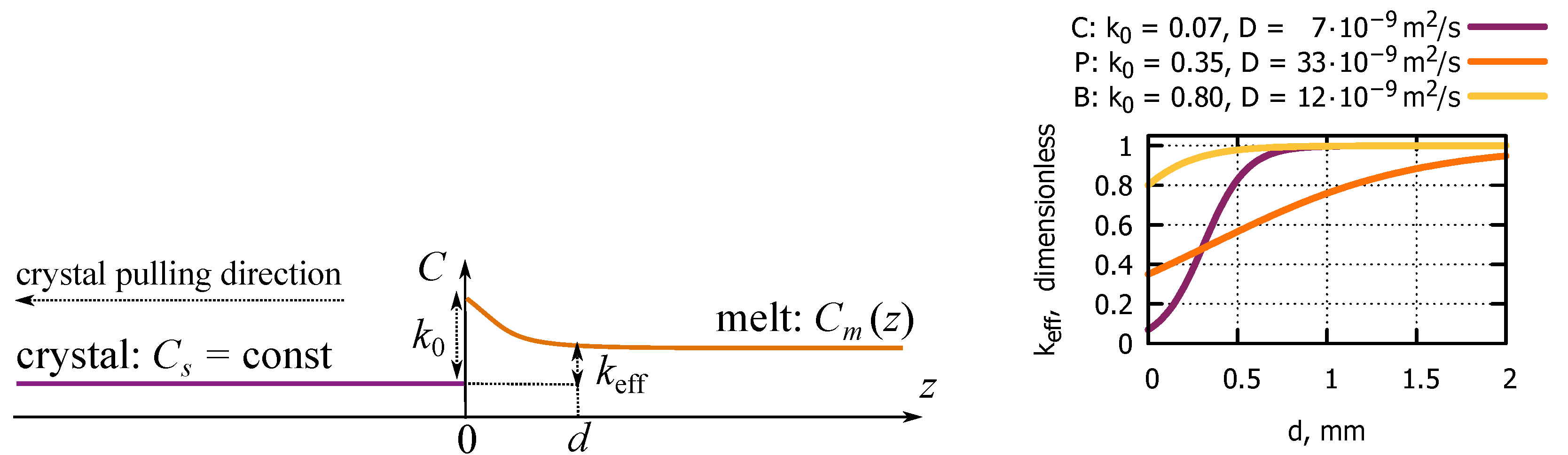
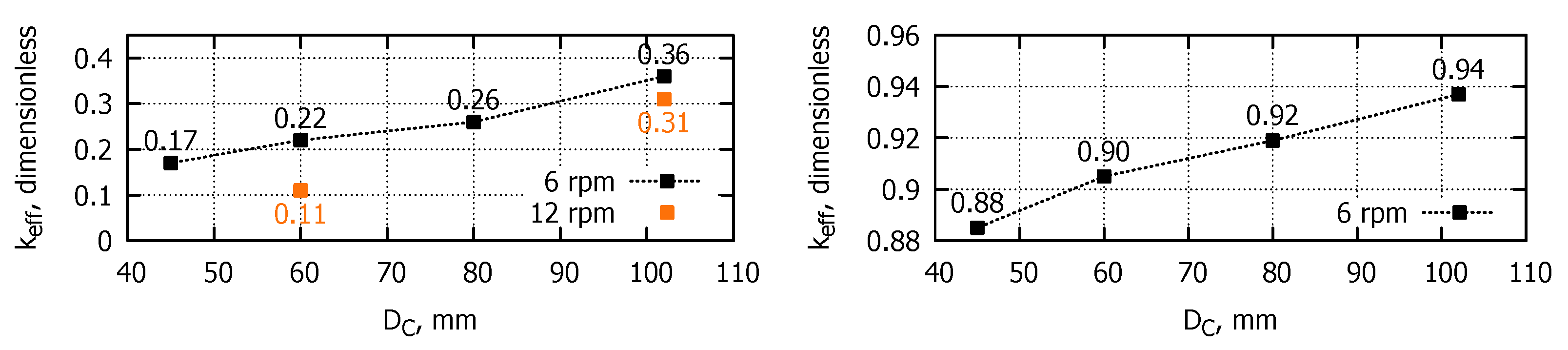
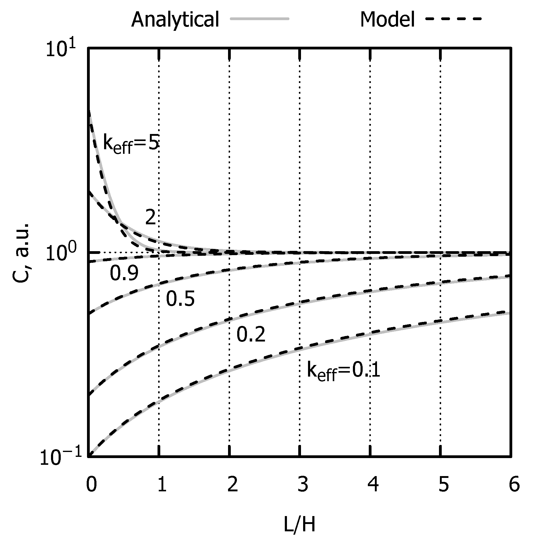
3.3.1. Effective Segregation Coefficient

From OpenFOAM melt flow simulations, the effective segregation coefficient can be calculated:

$$k_{\mathrm{eff}}=\frac{C_C}{C_m}=\frac{k_0{C}_{m,\mathrm{crys}.\mathrm{inter}.}}{C_m},$$

(5)

where $C_C$ is the concentration of species in the crystal, $C_m$ is the average species concentration in the melt, and $C_{m,\mathrm{crys}.\mathrm{inter}.}$ is the average species concentration on the crystallization interface, calculated by averaging the concentration values from the faces of OpenFOAM calculation cells.

Values of $k_{\mathrm{eff}}$ converged relatively rapidly—after less than 200 s, it did not change more than $\pm 2\%$. This means that, until the saturation of $k_{\mathrm{eff}}\left(t\right)$ curve, less than 12 mm of crystal is grown, which is a small part in comparison to total crystal length (400 mm and more). The obtained values of $k_{\mathrm{eff}}$ are summarized in Figure 16. The effective segregation coefficient monotonously increases as the crystal diameter increases. This can be explained by considering a simplified scheme in Figure 2: when $D_C$ is larger, the melt motion is less intensive, the boundary layer remains undisturbed, and the drop of species concentration in the melt is sharper. Therefore, $C_m(z\gg 0)$ becomes closer to $C_s$, and $k_{\mathrm{eff}}\equiv \frac{C_s}{C_m(z\gg 0)}$ increases.

The obtained range of carbon $k_{\mathrm{eff}}$ variation only partly intersects with the range calculated using the BPS model (1), where $k_{\mathrm{eff}}$ is in the interval from 0.3 to 0.5. This could possibly be explained by the simplifications during the derivation of the BPS model, which does not capture all features of the 3D melt flow in the FZ process. It should also be noted that the used carbon diffusion coefficient D is rather uncertain (its values are given in [28] with $\pm 30\%$ precision). The range of boron $k_{\mathrm{eff}}$, in turn, agrees with Equation (1) rather well.

The obtained $k_{\mathrm{eff}}$ value may depend on the used mesh due to the combination of extremely low D and low $k_0$ for carbon. During the research, mesh influence studies were performed, and it was shown that, in order to obtain consistent results, the cell size at the crystallization interface should not be larger than 0.03 mm in the normal direction. This criterion was ensured in all meshes that were used for the melt flow simulations described above.

3.3.2. Increased Crystal Rotation Rate

The crystal rotation rate ${\omega }_C$ was increased from 6 to 12 rpm in two stages—for $D_C=102\mathrm{m}\mathrm{m}$ and $D_C=60\mathrm{m}\mathrm{m}$—in order to investigate if it is possible to decrease carbon $k_{\mathrm{eff}}$ and thus improve the crystal purification. The comparison of meridional velocity fields revealed only small differences; see Figure 17. Vertical motion (downwards in the centre of the melt and upwards at the middle of the radius) became slightly stronger when ${\omega }_C$ was increased to 12 rpm.

Therefore, the central maximum in the radial distribution of the carbon concentration became more pronounced; see Figure 15 (dashed lines). As shown in Figure 16, an increase in ${\omega }_C$ from 6 to 12 rpm led to a decrease in $k_{\mathrm{eff}}$ from 0.36 to 0.31 for $D_C=102\mathrm{m}\mathrm{m}$ and decreased $k_{\mathrm{eff}}$ by half for $D_C=60\mathrm{m}\mathrm{m}$. This means that the high ${\omega }_C$ could help to achieve a slightly higher average crystal purity; however, an increase in the $C\left(r\right)$ profile maximum is predicted, as shown in Figure 15, which will make the 2D $C(r,z)$ distribution in the grown crystal less homogeneous.

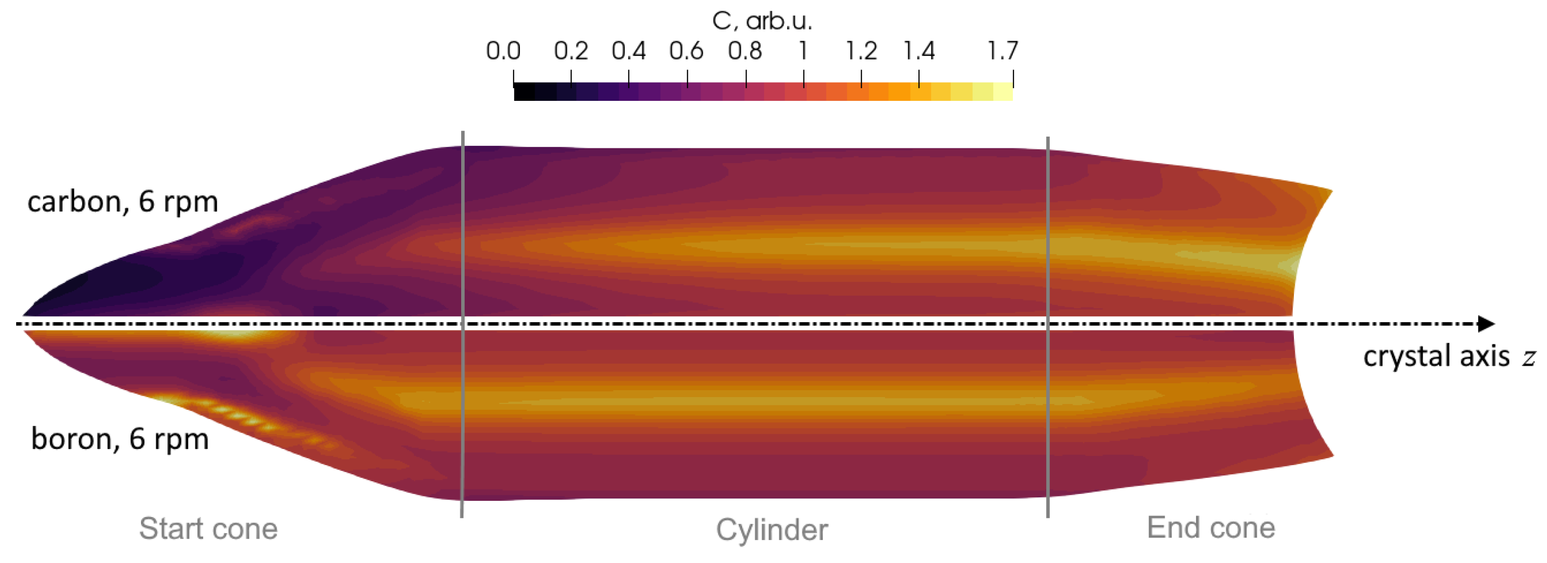
3.4. Species Distribution in Crystal

The developed program 0D-segregation, which calculates the axial distribution of impurities (Section 2.4), was verified using an analytical solution for a theoretical “cylindrical crystal”—a crystal with constant diameter, disregarding the cone phases. The results of the verification are presented in Appendix B.

A proper comparison with analytical expressions is only possible for the fully cylindrical system. In reality, the crystal diameter is not constant and includes cone stages at the beginning and the end of the growth process—the crystal diameter evolution is shown in Figure 9. For the cases when precise process data (either experimental logs or the output of the transient FZoneT program) is not available, the 0D-segregation program has a setting that creates a simplified crystal shape $D_C\left(L\right)$ as described in the end of Section 2.4. Figure 18 (left) shows this simplified shape for a 102 mm crystal: the crystal diameter and melt volume are functions of the crystal length and are compared with the shape simulated by FZoneT.

Changes in crystal diameter have a significant impact in the resulting species distribution in the crystal as shown in Figure 18 (right). In all cases, uniform carbon concentration in the feed rod is assumed. During the start cone stage, the melt volume increases, which causes a slower impurity build-up than in the analytically solved cylindrical crystal case.

The opposite effect can be seen during the end cone stage when the impurity concentration exceeds the initial values in the feed rod. Another reason for the difference between the cylindrical crystal and the real crystal is the $k_{\mathrm{eff}}$ dependence on the crystal radius, which was shown in Figure 16. The simplification of the crystal shape significantly impairs the precision of the obtained $C\left(L\right)$ distribution, which is likely due to the imprecise description of the melt volume.

The axial concentration distribution, which was obtained using the precise crystal shape simulated by FZoneT, was combined with radial distributions at corresponding diameters (shown in Figure 15), and linear interpolation was used between them. As a result, the 2D $C(r,z)$ distribution in the entire crystal is shown in Figure 19.

4. Discussion

A new model system was proposed to describe the transient FZ growth of silicon, including the shapes of the phase boundaries and the resulting species concentration in the crystal influenced by melt flow.

Simulations of the shapes of phase boundaries, both transient and quasi-stationary, corresponded well to the experimental data (process photographs, zone height and crystal diameter). The differences usually did not exceed 1–2 mm, which is sufficient to use the obtained phase boundaries and the calculated 3D electromagnetic field for further melt flow simulations.

The melt flow simulations demonstrated significant differences between stages with small ($D_C\le 65$ mm) and large ($D_C\ge 80$ mm) crystal diameters during the cone phase. In the small melts, the vortex induced by EM force occupied more than a half of the melt. In the large melts, on the contrary, intensive melt motion occurred only in the thin layer near the free melt surface.

Differences in the melt flow influence species transport significantly: two maximums in the radial concentration profile occurred for small crystal diameters but only one for large crystal diameters. The radial variation of concentration reached $\pm 50\%$ for carbon and $\pm 5\%$ for boron. The profile shapes were similar for both elements with larger variations obtained for small crystal diameters. The differences between the simulations and analytically predicted axial distribution are considerably large due to the effects of cone phases. It was also observed that the precise description of melt volume evolution is important for obtaining axial species distribution in the grown crystal.

The simulated values of the effective segregation coefficient $k_{\mathrm{eff}}$ qualitatively agree with the classical BPS model (the BPS model predicted 0.38–0.48 for carbon) and experimental data from other silicon growth processes (experimental results were 0.73–0.98 for boron). However, numerical simulations showed that $k_{\mathrm{eff}}$  increases for larger melt diameters due to less intensive melt motion. The increase in the crystal rotation rate from 6 to 12 rpm reduces $k_{\mathrm{eff}}$, particularly for small crystal diameters. These results are crucial for the accurate prediction of the species distribution in FZ Si crystals.

References

1. Mühlbauer, A.; Muiznieks, A.; Raming, G.; Riemann, H.; Lüdge, A. Numerical modelling of the microscopic inhomogeneities during FZ silicon growth. J. Cryst. Growth 1999, 198, 107–113. [Google Scholar] [CrossRef]
2. Abrosimov, N.V.; Aref’ev, D.G.; Becker, P.; Bettin, H.; Bulanov, A.D.; Churbanov, M.F.; Filimonov, S.V.; Gavva, V.A.; Godisov, O.N.; Gusev, A.V.; et al. A new generation of 99.999% enriched 28Si single crystals for the determination of Avogadro’s constant. Metrologia 2017, 54, 599–609. [Google Scholar] [CrossRef]
3. Sze, S.; Lee, M. Semiconductor Devices: Physics and Technology; John Wiley & Sons, Inc.: Hoboken, NJ, USA, 2012; p. 361. [Google Scholar]
4. Burton, J.A.; Prim, R.C.; Slichter, W.P. The distribution of solute in crystals grown from the melt. Part I. Theoretical. J. Chem. Phys. 1953, 21, 1987–1991. [Google Scholar] [CrossRef]
5. Priede, J.; Gerbeth, G. Breakdown of Burton-Prim-Slichter approach and lateral solute segregation in radially converging flows. J. Cryst. Growth 2005, 285, 261–269. [Google Scholar] [CrossRef] [Green Version]
6. Wilson, L.O. Analysis of microsegregation in crystals. J. Cryst. Growth 1980, 48, 363–366. [Google Scholar] [CrossRef]
7. Mühlbauer, A.; Muižnieks, A.; Virbulis, J. Analysis of the dopant segregation effects at the floating zone growth of large silicon crystals. J. Cryst. Growth 1997, 180, 372–380. [Google Scholar] [CrossRef]
8. Lācis, K.; Muižnieks, A.; Jēkabsons, N.; Rudevičs, A.; Nacke, B. Unsteady 3D and analytical analysis of segregation process in floating zone silicon single crystal growth. Magnetohydrodynamics 2009, 45, 549–556. [Google Scholar] [CrossRef]
9. Han, X.F.; Liu, X.; Nakano, S.; Kakimoto, K. Numerical analysis of dopant concentration in 200 mm (8 inch) floating zone silicon. J. Cryst. Growth 2020, 545, 125752. [Google Scholar] [CrossRef]
10. Sim, B.C.; Kim, K.H.; Lee, H.W. Boron segregation control in silicon crystal ingots grown in Czochralski process. J. Cryst. Growth 2006, 290, 665–669. [Google Scholar] [CrossRef]
11. Hong, Y.H.; Sim, B.C.; Shim, K.B. Distribution coefficient of boron in Si crystal ingots grown in cusp-magnetic Czochralski process. J. Cryst. Growth 2008, 310, 83–90. [Google Scholar] [CrossRef]
12. Mei, P.R.; Moreira, S.P.; Cortes, A.D.S.; Cardoso, E.; Marques, F.C. Determination of the effective distribution coefficient (K) for silicon impurities. J. Renew. Sustain. Energy 2012, 4, 043118. [Google Scholar] [CrossRef]
13. Series, R.W.; Hurle, D.T.; Barraclough, K.G. Effective distribution coefficient of silicon dopants during magnetic Czochralski Growth. IMA J. Appl. Math. 1985, 35, 195–203. [Google Scholar] [CrossRef]
14. Jeon, H.J.; Park, H.; Koyyada, G.; Alhammadi, S.; Jung, J.H. Optimal cooling system design for increasing the crystal growth rate of single-crystal silicon ingots in the Czochralski process using the crystal growth simulation. Processes 2020, 8, 1077. [Google Scholar] [CrossRef]
15. Ding, J.; Li, Y.; Liu, L. Effect of cusp magnetic field on the turbulent melt flow and crystal/melt interface during large-size Czochralski silicon crystal growth. Int. J. Therm. Sci. 2021, 170, 107137. [Google Scholar] [CrossRef]
16. Ratnieks, G.; Muižnieks, A.; Mühlbauer, A. Modelling of phase boundaries for large industrial FZ silicon crystal growth with the needle-eye technique. J. Cryst. Growth 2003, 255, 227–240. [Google Scholar] [CrossRef]
17. Rudevičs, A.; Muižnieks, A.; Ratnieks, G.; Mühlbauer, A.; Wetzel, T. Numerical study of transient behaviour of molten zone during industrial FZ process for large silicon crystal growth. J. Cryst. Growth 2004, 266, 54–59. [Google Scholar] [CrossRef]
18. Lācis, K.; Muižnieks, A.; Rudevičs, A.; Sabanskis, A. Influence of DC and AC magnetic fields on melt motion in FZ large Si crystal growth. Magnetohydrodynamics 2010, 46, 199–218. [Google Scholar]
19. Ratnieks, G.; Muiznieks, A.; Buligins, L.; Raming, G.; Mühlbauer, A.; Lüdge, A.; Riemann, H. Influence of the three dimensionality of the HF electromagnetic field on resistivity variations in Si single crystals during FZ growth. J. Cryst. Growth 2000, 216, 204–219. [Google Scholar] [CrossRef]
20. Surovovs, K. A Program for Calculating Dopant Concentration Distribution in a Crystal Grown in Float-Zone Process. Available online: https://git.lu.lv/ks10172/zero-d (accessed on 30 September 2022).
21. Muižnieks, A.; Rudevics, A.; Riemann, H.; Lacis, U. Comparison between 2D and 3D modelling of HF electromagnetic field in FZ silicon crystal growth process. In Proceedings of the International Scientific Colloquium Modelling for Material Processing, Riga, Latvia, 16–17 September 2010; pp. 61–65. [Google Scholar]
22. Muižnieks, A.; Lacis, K.; Nacke, B. 3D unsteady modelling of the melt flow in the FZ silicon crystal growth process. Magnetohydrodynamics 2007, 43, 377–386. [Google Scholar] [CrossRef]
23. Sabanskis, A.; Surovovs, K.; Virbulis, J. 3D modeling of doping from the atmosphere in floating zone silicon crystal growth. J. Cryst. Growth 2017, 457, 65–71. [Google Scholar] [CrossRef]
24. Ribeyron, P.; Durand, F. Oxygen and carbon transfer during solidification of semiconductor grade silicon in different processes. J. Cryst. Growth 2000, 210, 541–553. [Google Scholar] [CrossRef]
25. Rost, H.J.; Menzel, R.; Luedge, A.; Riemann, H. Float-Zone silicon crystal growth at reduced RF frequencies. J. Cryst. Growth 2012, 360, 43–46. [Google Scholar] [CrossRef]
26. Surovovs, K.; Muiznieks, A.; Sabanskis, A.; Virbulis, J. Hydrodynamical aspects of the floating zone silicon crystal growth process. J. Cryst. Growth 2014, 401, 120–123. [Google Scholar] [CrossRef]
27. Mills, C.; Courtney, L. Thermophysical Properties of Silicon. ISIJ Int. 2000, 40, 130–138. [Google Scholar] [CrossRef]
28. Eremenko, V.N.; Gnesin, G.G.; Churakov, M.M. Dissolution of polycrystalline silicon carbide in liquid silicon. Test Methods Prop. Mater. 1972, 11, 471–474. [Google Scholar] [CrossRef]
29. Garandet, J.P. New determinations of diffusion coefficients for various dopants in liquid silicon. Int. J. Thermophys. 2007, 28, 1285–1303. [Google Scholar] [CrossRef]
30. Kolbesen, B.O.; Mühlbauer, A. Carbon in silicon: Properties and impact on devices. Solid-State Electron. 1982, 25, 759–775. [Google Scholar] [CrossRef]
31. Menzel, R. Growth Conditions for Large Diameter FZ Si Single Crystals. Ph.D. Thesis, Technischen Universität, Berlin, Germany, 2013. [Google Scholar]
32. Milliken, K.S. Simplification of a molten zone refining formula. J. Met. 1955, 7, 838. [Google Scholar] [CrossRef]
Figure 1. Axially symmetrical scheme of the FZ method, with designations of the most important parts and the used coordinate system.
Crystals 12 01718 g001
Figure 2. Left—a simplified scheme of species distribution in the crystal ( z < 0 ) and the molten zone ( z > 0 ) near the interface ( z = 0 ). Right—the dependence of the effective segregation coefficient k eff on diffusion layer thickness d (e.g., [4]) for different species [16,17,18,19].
Crystals 12 01718 g002
Figure 3. The overall scheme of the used numerical models (orange boxes) and the data that is being exchanged between them (grey boxes).
Crystals 12 01718 g003
Figure 4. The scheme of species concentration interpolation from OpenFOAM melt flow simulations of the cone stage and cylinder stage (a) and 0D-segregation simulations (b) on the grown crystal mesh (c).
Crystals 12 01718 g004
Figure 5. 3D high-frequency electromagnetically induced heat sources on silicon surfaces used for 3D melt flow simulations. The one-turn inductor is shown in grey.
Crystals 12 01718 g005
Figure 6. Comparison of induced currents on silicon surfaces in the case of 2D and 3D simulations.
Crystals 12 01718 g006
Figure 7. Comparison between shapes of the phase boundaries for optimized 2D and 3D EM simulations.
Crystals 12 01718 g007
Figure 8. Comparison of the shapes of phase boundaries in the transient FZoneT simulation with experimental photos during the cone growth (0–30 min) and cylindrical growth (40 min) stages.
Crystals 12 01718 g008
Figure 9. Comparison of transient FZoneT simulation results to the experiment during the entire growth process.
Crystals 12 01718 g009
Figure 10. The time-averaged meridional melt velocity in the x z plane, temperature in the y z plane and carbon concentration on the crystallization interface, simulated for the cylindrical phase ( D C = 102 mm). The direction of the main inductor current suppliers corresponds to the x axis.
Crystals 12 01718 g010
Figure 11. The time-averaged melt velocity (left) and carbon concentration (right) in the vertical cross-section of the melt, simulated for the cylindrical phase ( D C = 102 m m ) and cone phase ( D C < 102 m m ).
Crystals 12 01718 g011
Figure 12. Absolute values of the EM and Marangoni force density on the free melt surface during the cylindrical phase ( D C = 102 m m ).
Crystals 12 01718 g012
Figure 13. The distribution of carbon (left) and boron (right) concentration in the melt, near the crystallization interface ( D C = 102 m m ). The normal coordinate is denoted by n, and different radial positions r are considered. Boundary layer thicknesses from the BPS model (1) are shown with vertical black lines.
Crystals 12 01718 g013
Figure 14. The time-averaged carbon concentration on the crystallization interface, simulated for the cone phase ( D C < 102 m m ) and cylindrical phase ( D C = 102 m m ).
Crystals 12 01718 g014
Figure 15. Normalized radial distributions of carbon (left) and boron (right) concentrations in the grown crystal (yellow line for the cylindrical phase, violet and orange lines for the cone phase), using crystal rotation rates 6 rpm (solid lines) and 12 rpm (dashed lines).
Crystals 12 01718 g015
Figure 16. The effective segregation coefficient k eff of carbon (left) and boron (right) obtained for different crystal diameters D C and crystal rotation rates of 6 rpm (black) and 12 rpm (orange).
Crystals 12 01718 g016
Figure 17. The time-averaged melt velocity in the vertical cross-section of the melt, simulated for the cylindrical phase with D C = 102 m m and crystal rotation rates of 6 rpm (left) and 12 rpm (right).
Crystals 12 01718 g017
Figure 18. The crystal diameter and melt volume as a function of the crystal length L for the considered D C = 102 mm system with cone stages (left) and comparison of the axial carbon concentration in the crystal using different crystal shapes with k eff ( D C ) from the melt flow simulation results (right). Vertical grey lines represent the boundaries between the start cone, cylinder and end cone stages.
Crystals 12 01718 g018
Figure 19. An example of the carbon and boron distribution in the grown crystal (top) and the axial distribution of radially averaged concentration of these species (bottom).
Crystals 12 01718 g019aCrystals 12 01718 g019b