Predicting the Crystal Structure and Lattice Parameters of the Perovskite Materials via Different Machine Learning Models Based on Basic Atom Properties

Abstract

Perovskite materials have high potential for the renewable energy sources such as solar PV cells, fuel cells, etc. Different structural distortions such as crystal structure and lattice parameters have a critical impact on the determination of the perovskite’s structure strength, stability, and overall performance of the materials in the applications. To improve the perovskite performance and accelerate the prediction of different structural distortions, few ML models have been established to predict the type of crystal structures and their lattice parameters using the basic atom characteristics of the perovskite materials. In this work, different ML models such as random forest (RF), support vector machine (SVM), neural network (NN), and genetic algorithm (GA) supported neural network (GA-NN) have been established, whereas support vector regression (SVR) and genetic algorithm-supported support vector regression (GA-SVR) models have been assessed for the prediction of the lattice parameters. The prediction model accuracy for the crystal structure classification is almost 88% in average for GA-NN whereas for the lattice constants regression model GA-SVR model gives ~95% in average which can be further improved by accumulating more robust datasets into the database. These ML models can be used as an alternative process to accelerate the development of finding out new perovskite material by providing valuable insight for the behaviours of the perovskite materials.

1. Introduction

Due to its attractive material characteristics with superconductivity, catalytic activity, and ionic conductivity, perovskite is used in a diverse range of uses together with fuel cells and solar cells [1,2,3]. For crystalline solids, the crystal structure and associated lattice constants play a key role in predicting the physical properties [4]. A perovskite is described by an ABX₃ stoichiometry where: A is a large cation such as a rare earth (La, Pr, Nd, Sm, Eu, Gd, etc.) or alkaline ion (Ca, Sr, Ba, etc.); B is a transition metal ion (Cr, Mn, Fe, Sc, Ni, Co, etc.); and X is an oxide or halide [5,6,7,8]. Perovskites have a large flexibility regarding A and B site chemical substitutions and as such can have a cubic, monoclinic, tetrahedral, hexagonal, or rhombohedral crystal structure.

Generally, the cubic structure is considered the ideal crystal structure for the ABO₃ type perovskite materials. In the cubic perovskite crystal structure, the 3D framework contains corner sharing BO₆ octahedra (Figure 1). The A-cation is enclosed by 12 equidistant atoms [9,10]. The O anions have a coordination number of two (two B cations). The coordination number of the O anion is low, as the A-O distance is almost 40% greater than the B-O bond distance.

The mismatch of the cube–octahedral cavity size and constituent ionic radii are the causes for the deviation in the crystal structure especially from the cubic structure [11]. The distortion from the standard cubic structure are ascribed to three basic reasons: (1) BO₆ octahedra tilt (such as CrO₆/MnO₆), (2) distortions from polar cations, (3) octahedra distortion due to Jahn–Teller distortion [12]. The deviation from an ideal cubic structure can be estimated by the Goldschmidt tolerance factor, t = (R_A + R_O)/(√ 2 [R_B + R_O]) where R_A, R_B, and R_O are the radii of A-site cation, B-site cation, and O anion, respectively [13]. If the tolerance factor is close to unity, it is predicted that the perovskite should have a cubic structure. For 0.96 < t < 1, the perovskites are predicted to have a rhombohedral structure, and for t < 0.96, the perovskites are predicted to have an orthorhombic structure. Greater deviations from unity (t > 1) lead to perovskites with a hexagonal structure [14].

The reduced distortion in a cubic perovskite structure is the building block for good oxide ion conductivity—as required in fuel cell applications. Density functional theory (DFT) can be used to predict the crystal structure and lattice parameters to a relatively high accuracy. However, this is still time consuming. There are already large crystal structure databases for various materials. Using machine learning (ML) methods, these databases can be interrogated to predict the crystal structure and lattice parameters of new perovskite materials.

Recently, one research work has been reported for the classification of the crystal structure of ABO₃ type perovskites using Light GBM algorithm (2020) [17]. Santosh and Taher et al. reported that they have successfully implemented this model on 675 compounds out of 5329 ABO₃ perovskites and obtained 80.3% accuracy for this modelling system. However, in their work, the accuracy can be further improved if there is no over sampling issue with the proposed modelling system. Some other researchers (Evgeny et al., 2019) have tried a new combining approach to predict the crystal structures of different materials such as carbon, boron allotropes, and sodium (which contains high pressure phases) [18] by establishing a model which comes from the combination of USPEX (an evolutionary algorithm) and learning on-the-fly (which is an active learning method). They have achieved an accuracy of 11 meV/atom for the boron and its allotrope which is very promising, but they have not reported the prediction accuracy rate of their modelling system for the ABO₃ type perovskites in their works. On the other hand, in their modelling system, their method was actually relaxed with DFT.

In another current work, researchers have proposed ML models for determining the crystal system and space group prediction of materials from their composition only [19]. They combined RF and MLP neural network models using three kinds of features such as Magpie, one-hot encoding, and atom vector. Their results reported that RF combined with Magpie performs excellently compared to other algorithms for binary and multiclass prediction of crystal systems and space groups. However, the best Matthews correlation coefficient (MCC) scores are 0.591 and 0.627, respectively, for their prediction model. From the model outputs, it can be assumed that their ML algorithms and descriptors are not good enough to achieve suitable performance, which leads the other researchers to go for considering more conventional algorithms.

In the literature, there is limited work completed on the classification of crystal structures. Shandiz et al. (2016) [20] attempted to find out the important features for different crystal structures of cathodes composited with the Li–Si–(Mn, Fe, Co)–O configurations. In their work, mainly three crystal structures (monoclinic, triclinic, and orthorhombic) of silicate-based cathodes were predicted using various ML classification algorithms based on the DFT-generated database. They concluded that RF and extremely randomized trees provided the best performance model. They used Monte Carlo cross validation system for the validation process. They have mentioned their limitations as the limited available datasets of the silicate cathode materials, which can affect the performance of the models significantly.

Several groups have investigated methods to predict lattice parameters of inorganic crystalline materials in the literature. Recently, Ibrahim et al. (2020) have reported to establish an ML (SVR) model for the prediction of the lattice constant of the A₂XY₆ type cubic crystals (A = K, Cs, Rb, TI; X = tetravalent cation; and Y = F, Cl, Br, I) of the form A₂XY₆ (A = K, Cs, Rb, TI; X = tetravalent cation; and Y = F, Cl, Br, I) [21]. Their results for the prediction of lattice parameter A presented a high relationship of 99.87% for the training and 99.57% for the testing phase. To prove the robustness of the model, their developed model was compared with the previous existing linear model for 26 cubic crystal samples and the outcome showed a comparative deviation of 1.757 for the SVR model and 2.704 for the linear model. However, their database was very small with 85 samples which keeps a scope for further investigation considering for a larger dataset, and they have not reported for other lattice parameters prediction capability also by their model.

In another recent research work, they reported that their RF model with a novel descriptor for the prediction of lattice constants outperforms as an average R² score of 0.973 for ‘a’ lattice parameter of cubic crystal, compared to 0.80 for all other crystal systems [22]. They have also measured the prediction model accuracy for the lattice parameters b and c, which was lower comparatively than ‘a’ lattice parameter prediction accuracy in terms of R² score between 0.498 and 0.757. Though their model gives a comparatively high accuracy for a larger database system of 125,278 datasets of different crystal structures, they have not clearly mentioned about the reason behind the prediction model’s different accuracy for three lattice constants (a, b, c) of the same crystal structures.

In an early piece of work, Javed et al. (2007) established a model for lattice constant prediction using an SVR method [23]. They investigated the model generalizability using a four-fold cross-validation method through 157 samples for training and validation purpose and four samples for testing module. Their average absolute error was less than 0.7% for the training and validation models, and for testing model it was less than 0.6%. They compared the SVR results with an ANN model. Though the SVR prediction models gave higher accuracy for a small number of datasets, there was no discussion about the accuracy for a large dataset in their work, which need to be further investigated.

In 2010, Majid et al. implemented [24] SVM, ANN, and GRNN models, which achieved lower mean percentage absolute difference (PAD) values of 0.476% for SVM, 0.647% for ANN, and 0.565% for GRNN during the prediction of the lattice parameters of cubic type perovskites. Similarly, for the validation test, the SVR showed low PAD value as 0.088%, whereas ANN showed 0.662%, and GRNN showed 0.182%, correspondingly. They concluded that the SVR model provided a more accurate prediction (to achieve PAD values ~0.000%) than the GRNN and ANN models. However, they have also the same limitations as others of using limited datasets of only 132 cubic perovskites, which proves the necessity of further exploration of this study.

The crystal structure largely depends on the density of states (DOS) [25]. The DOS of a material is typically predicted using DFT. Schütt et al. (2014) predicted the DOS using a partial radial distribution function (PRDF). Although the accuracy of this work needs further improvement, this provided a method to screen a large number of materials. However, the average error was smaller than 6% compared to the DOS proper value range. Their results reveal that an accelerated prediction for solid material’s electronic attributes is possible using ML algorithms. This work involves an initial screening by using ML models followed by a detailed electronic structure (DFT) calculation. They have found that the performance of the prediction model was largely affected by the representation of the crystals.

Many other researchers are currently working on the possibility of using different ML models to save their time, cost, and energy to know the optimization of newly predicted materials or tools in their field such as Ammar and Niaz (2021) [26], who have tried ANN, NLR, and ANFIS models to find out the suitability of using rice husk ask as a concrete material instead of cement, which contribute largely to produce carbon dioxide into the environment, causing global warming issues. Another research work conducted by Fahid and Mohamed (2021) [27] also shows the prediction efficiency of GEP model to measure the compressive strength of rice husk ash for concrete purposes. However, both of the research works have considered a small number of datasets, which shows a path of investigating furthermore deeply for their works.

Although the Goldschmidt tolerance factor provides a good general rule for determining the perovskite crystal structure, in many cases it does not provide an accurate prediction. Recently, the authors [28] projected a model for the prediction of the lattice parameters of cubic perovskites ABX₃ using average ionic radii (R_av) of ABX₃. They have explored the regularities leading perovskites’ construction through an empirical structural map method using only 173 perovskite oxide systems. They have concluded that the octahedral factor (R_B/R_O) is as significant as the Goldschmidt tolerance factor, with regard to the formability of perovskites which need to be further investigated for a larger number of perovskite materials.

In an earlier study, Oganov et al. (2006) established an effective method for the crystal structure prediction through combining ab initio total-energy calculations with an evolutionary algorithm [29]. They reported a high success rate (ca. 100%) for the few tests (around tens) including ionic, metallic, covalent, and molecular structures containing up to 40 atoms in a unit cell. They have used temperature, pressure, hard constraints of the atoms, etc. The current restriction of their method was to order the periodic structures, which could be possibly overcome by calculating the free energies of disordered and aperiodic structures.

New and emerging databases provide an excellence source of data from which researchers can explore the use of ML algorithms. Emery and Wolverton (2017) [16] presented an integrated dataset of 5329 cubic and distorted perovskites, which were collected from experimental observation and from first principle DFT calculations. This large dataset comprises of 395 perovskites for the prediction of thermodynamically stable perovskites but have not been defined yet by experiment based on their selected features from the available datasets.

Several ML models are being proposed for the prediction of the lattice parameters and the crystal structures of various materials—including perovskites. However, all the work reported ([20], etc.) on perovskite crystal structure and lattice constant prediction are limited to small datasets. There is also scoped to modify their model feature engineering and model accuracy for further improvement. Computational prediction of crystal structure and lattice parameters of perovskite materials has a widespread implementation in property investigation and performances for renewable energy sources especially for FC, solar cells, etc. In this work, we use a large ABO₃ perovskite database to establish an ML algorithm that can accurately predict the crystal structure and lattice parameter from basic atom characteristics. Different ML algorithms are used to establish a suitable ML model. For crystal structure classification, GA assisted NN model provides the best accuracy. For prediction of lattice parameters, a genetic algorithm optimized support vector regression (SVR-GA) model provides the best accuracy. However, the model accuracy is limited due to their inability to interpretation the nonlinearity in the atomic level properties and lattice parameters correlation.

2. Modelling Strategy

The main aims of this work are to build (1) an ML model which can classify different crystal structures of ABO₃ perovskites and (2) an efficient regression model to predict the ABO₃ perovskite lattice parameters. In both cases, the basic atom characteristics have been used as the input features.

For both subtasks the same workflow is used:

(i)

Database construction—to develop a database system

(ii)

Feature selection.

(iii)

Data pre-processing.

(iv)

Hyper-parameter optimization—ML model tuning.

(v)

Testing model for accuracy.

Figure 2 shows the prediction framework for the targeted properties of ABO₃ perovskites in the present study.

2.1. Model Environment

Python 3 was the programming language for this project. For the SVM and RF models, Scikit-learn [30] was the chosen framework. Pandas [31] library tools are used for the data processing due to their ability for complicated data analysis efficiently along with fast data manipulation ability. Matplotlib [32] is utilized to cope with the visualization part.

2.2. Methods and ML Process

In this section, the database construction and data pre-processing steps will be introduced. Subsequently, the investigated machine learning models processing strategy will be briefly discussed.

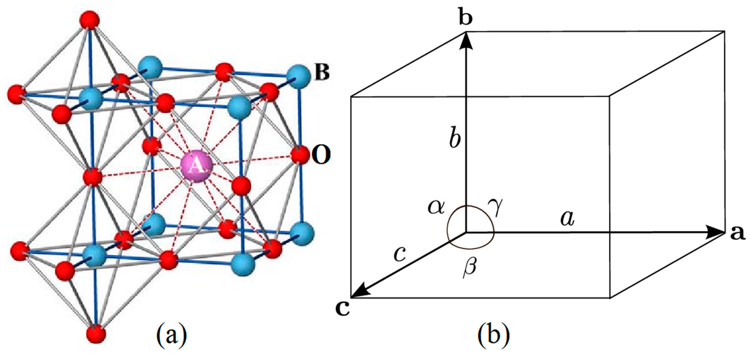
2.2.1. Database Construction

The database considered for this project is accumulated from the study work of Emery and Wolverton [33]. From their database, 2225 datasets have been chosen. No null or unknown values have been used in the current database. This dataset contains 222 experimental datasets and 2003 theoretical datasets (from the DFT calculation). In our work, we have considered the experimental datasets and DFT-calculated datasets equally as there are shortages of available experimental datasets for only ABO₃ type perovskite materials. Moreover, our main aim for this work is to establish an efficient model which can help researchers in the future to categorize any perovskite materials into the ABO₃ type classification and predict its lattice constants of any crystal structure based on basic atomic characteristics without using any experimental information.

Table 1. Current database features and labels for the project.

Feature List (Basic Atom Characteristics)	Label for Classification Models (Different Crystal Structures)	Label for Regression Models (Lattice Parameters)	Experimental Datasets	DFT Calculated Datasets
Atomic number of A site	Cubic	Lattice parameter A	222	2003
Atomic number of B site	Rhombohedral	Lattice parameter B
Atomic mass of A site	Tetragonal	Lattice parameter C
Atomic mass of B site	Orthorhombic
Valance of A site
Valance of B site
Ionic radii of A site
Ionic radii of B site
Electronegativity of A site
Electronegativity of B site
Polarizability of A site
Polarizability of B site
Total number of Datasets	2225	2225

shows the features and labels for the collected datasets. The features in the dataset include the atom number, atomic mass, valence, ionic radii, electronegativity, and polarizability for both the A and B atom. Features are selected based on the fundamental atomic and crystallographic properties of the available large ABO₃ type perovskite datasets found from the literature reviews according to their physical importance to the output variable. The same input features are used for both the crystal structure classification and the lattice parameter determination whereas the model outputs labelling is different for classification and regression models.

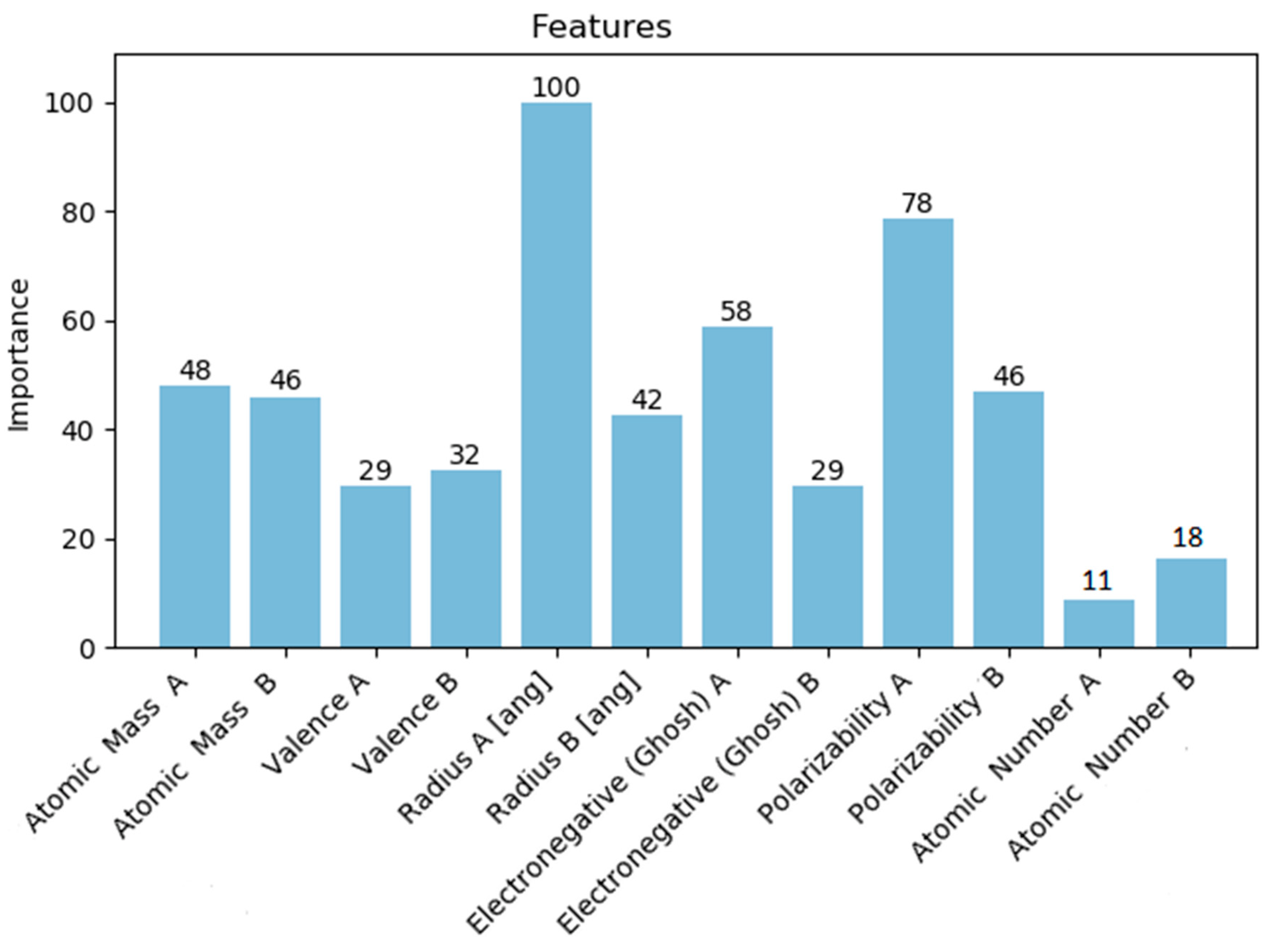
2.2.2. Feature Selection

In this work, a random forest (RF) algorithm is used to select the appropriate input features and to assess the variable importance (VI) of features. RF algorithm works based on an ensemble method consisting of a huge number of individual decision trees. Each decision tree includes its spits out vector values within the same level of distribution [28]. The process of calculating VI of features have been described in the Supporting Information (SI) S2 section. Using the VI evaluation measurements, it can be possible to find out the relationship among features and targeted labels [32]. Figure 3 shows the VI for the various atom features. These VI values are normalized between 0 to 100. Clearly the ionic radii of the A site element is the most important feature. However, all the features show some importance. The two least important features, atomic number of A and B, have been excluded from the datasets but all other input features are believed vital in predicting the crystal structure and the lattice parameter.

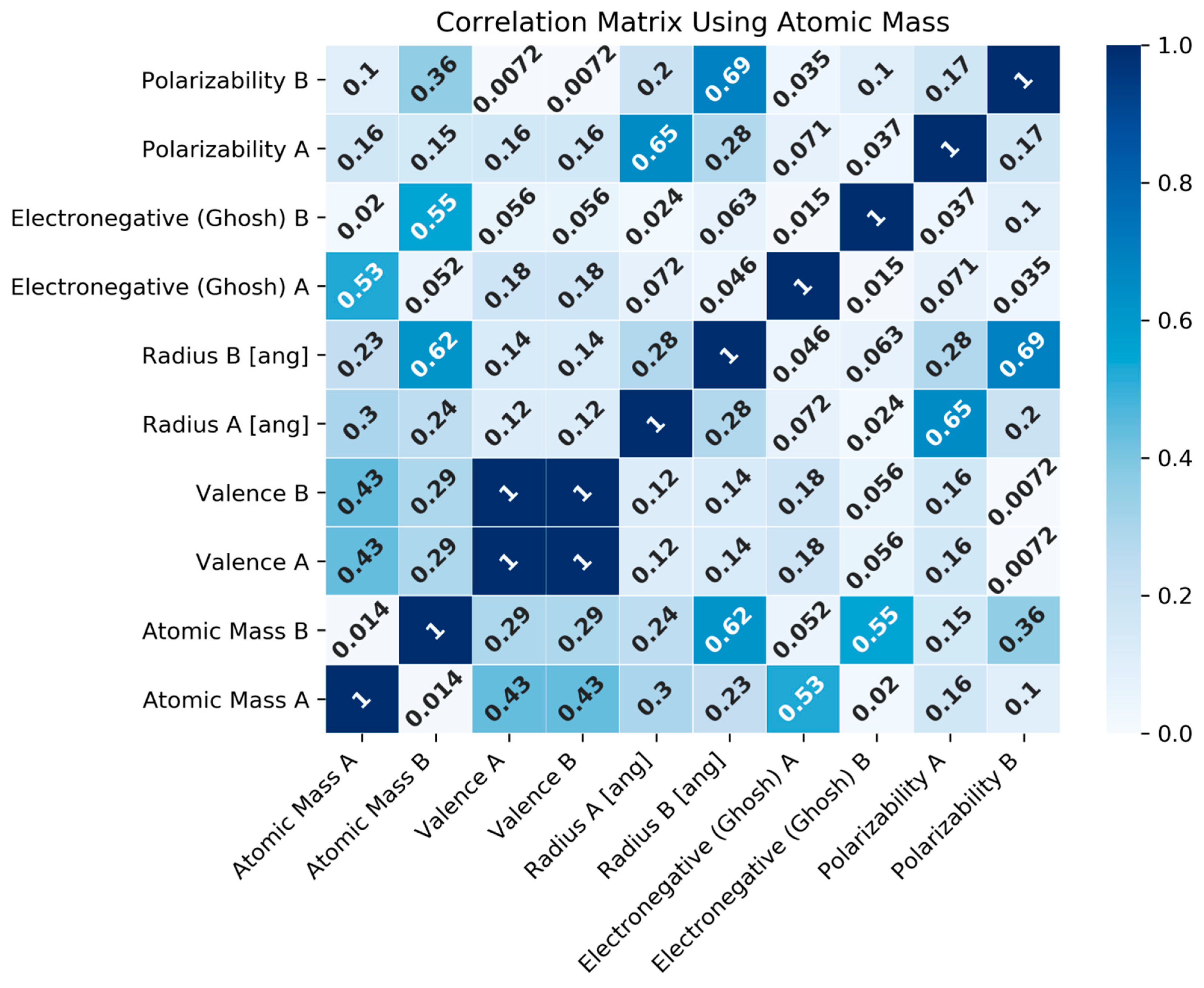
2.2.3. Feature Correlation

The datasets may contain recurring features. Pearson correlation coefficient matrix (R) can help to remove the repetitive features from the datasets as well as indicate the correlation importance between the features in terms of −1 to 1 value. It can be measured through the formula [34] described in the S3 Section of the SI briefly.

Figure 4 shows the Pearson correlation matrix for different features. Absolute values are considered for the negative values to show the correlation importance between features. Comparatively high values suggest high correlation between two features. A correlation of 1 indicates that they have the same importance or have a higher correlation between each other. In opposition, a comparatively low number indicates little correlation between two features. For instance, valence A and B gives a relatively high correlation (1) between each other because it balances the chemical formation of the crystal structure. However, a smaller value does not always mean unnecessity for removing any feature from the datasets as these features may contribute some other significance for the model. Therefore, all the features are considered important for establishing the prediction model of the crystal structure.

2.2.4. Feature Scaling

Feature scaling is a usual data pre-processing (DP) process for numerical features, especially when all features have different magnitudes, ranges, or units inducing a skewed correlation map. The two most common feature scaling methods are Normalization and Standardization. Adequate normalization or standardization accelerates the training process as well as reduces the error of the prediction models [35]. In the current datasets, almost all feature values are of different scales and units. Hence, normalization or standardization of numerical features is necessary to improve the data integrity by using the standard normalization techniques mentioned in the S4 Section of the SI [36]. Normalization helps to train a model more sophisticatedly by improving the mathematical calculation during optimization and can easily compare features with each other, which uses different scales previously for the measurement.

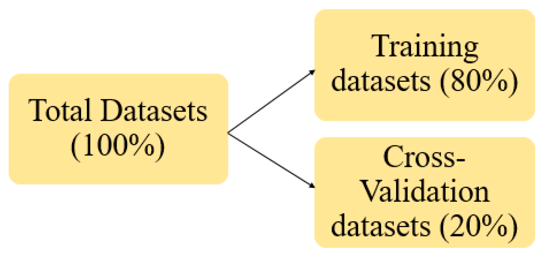
2.2.5. Datasets Pre-Processing (DP)

The datasets for this study consist of four different crystal structures: cubic, rhombohedral, tetragonal, and orthorhombic. For the ABO₃ perovskite materials in the database, there are three lattice parameters (a, b, and c) and three angles (α, β, and γ). The crystal structures can be defined by a combination of the lattice parameters and the lattice angles. For example, for the cubic crystal structure, a = b = c and all the lattice angles are 90° (

Table 2. Crystal structure representation.

Model Output Parameters (Different Crystal Structure)	Model Output Values for Crystal Structures	Lattice Parameters Mapping	Number of Collected Datasets
Cubic	0	$a=b=c$ α = β = γ = 90°	1379
Rhombohedral	1	$a=b=c$ α = β = γ$\ne$90°	131
Tetragonal	2	$a=b\ne c$ α = β = γ = 90°	64
Orthorhombic	3	$\mathrm{a}\ne \mathrm{b}\ne \mathrm{c}$ α = β = γ = 90°	651

).

To predict the crystal structures, these categorical labels need to be encoded into numerical values. This can be done using different encoding methods. There are several known encoding methods such as binary encoding, ordinal label encoding, one-hot encoding, etc., which are commonly used during modelling time. If each unique feature is categorized orderly by integer number, this is known as ordinal label encoding, whereas binary encoding translates the numbers into binary format, which is then separated into columns based on the dimension of numbers. One-hot encoding is mostly used for unordered structures. In this work, ordinal label encoding has been used where each category is given an integer value from 1 to N (where N is the number of categories related to the features). Table 2 shows the label encoding of the different crystal structures and the number of datasets available for each crystal structure type in the current database system.

From the 2225 datasets, 1379 are cubic, 651 are orthorhombic, 131 are rhombohedral, and 64 are tetragonal. This shows that the database is imbalanced. Such a large imbalance can have a major impact on the ML algorithm. For establishing an efficient modelling system, sufficient data have been considered from the database though there were also few bad data or ‘noise’ in the database. For all ML work, the dataset is split randomly into two parts: training (80%) and cross-validation (20%) modules (Figure 5). In the processed database, all datasets are quantified through a proper way for the modelling system.

3. Machine Learning Models

As mentioned earlier, one of the main aims of this work is to build:

A model for the classification of different ABO₃ perovskites crystal structures and an efficient regression model to predict the ABO3 lattice parameters.

In this section, the classification models used to predict the crystal structures will be introduced followed by the models used to predict the ABO₃ lattice parameters.

3.1. Crystal Structure Prediction Models

The prediction of a material’s crystal structure is important in searching for new ABO₃ perovskite materials. The hypothetical prediction of crystal structures is difficult because of the classification of energy minima on the energy surface of lattice constants. Due to the noteworthy improvement in the computational and theoretical field of materials, currently, it is conceivable to predict the structure of different crystals more conveniently. In this work, several machine learning algorithms have been implemented including RF, SVM, NN, and GA. In the following sections, the machine learning model is initially introduced followed by methods to tune these models.

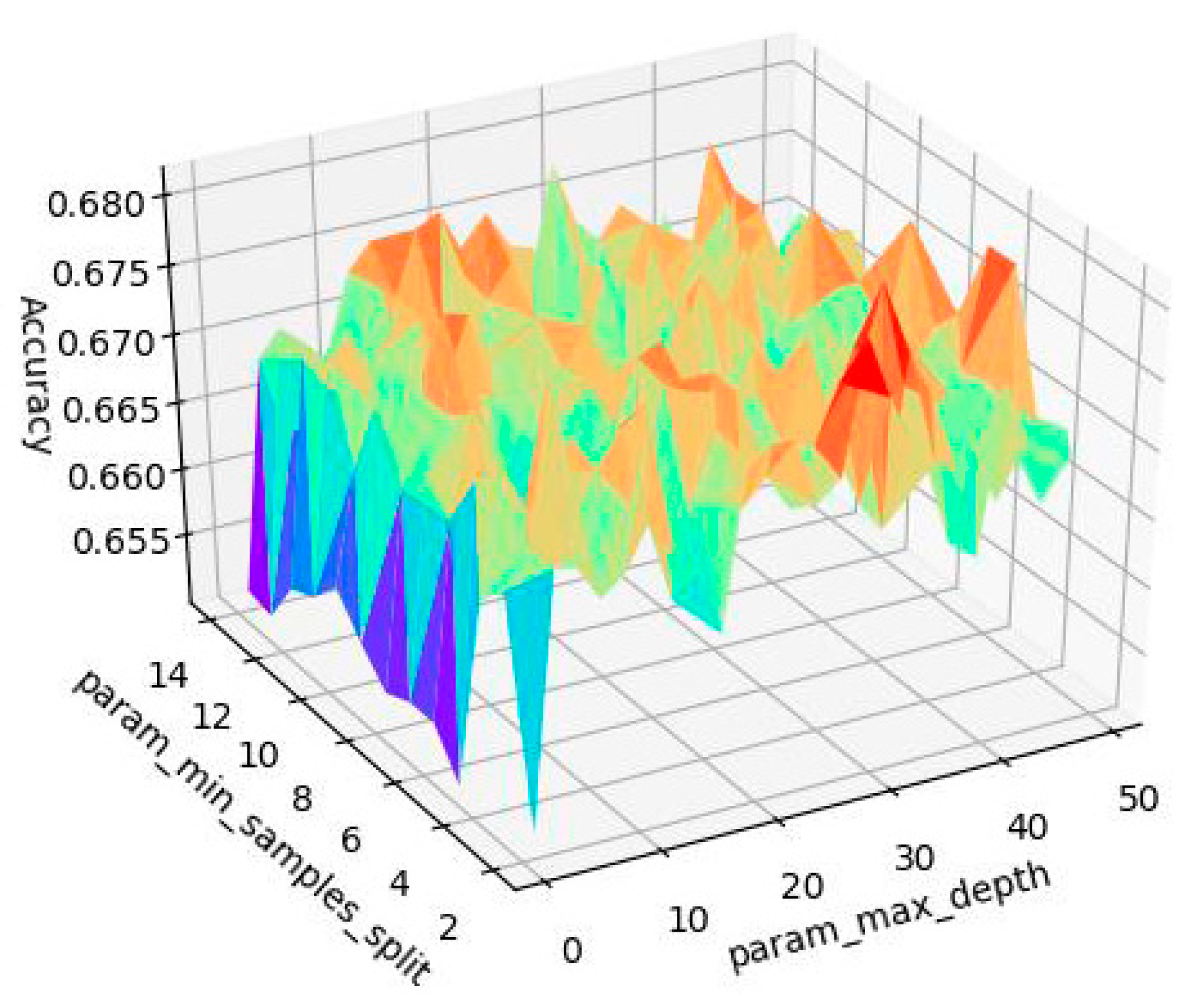
3.1.1. Random Forest—Modelling Process

Random forest (RF) is an ensemble method based on decision trees. RF uses different trees for different features based on the randomize selection process which provides different classifications. RF model’s output is decided through a balloting system. The ‘n_estimators’ parameter decides the number of trees needs to be generated for the RF model. More estimators could help to achieve an improved generalizability.

Random Forest—Model Tuning

Tuning is important to ensure that the model accurately predicts the validation set. In the RF modelling system, two hyperparameters such as maximum depth and minimum num of split of trees are challenging to define in RF modelling. A specific value is constrained for every estimator as the maximum depth of the tree so that when it goes to that specific value, it will stop to create new nodes further. The minimum sample split defines how many nodes each evaluation could generate. For a usual decision tree, its maximum depth is unlimited whereas the minimum sample split is generally 2. To obtain the appropriate value of maximum depth and minimum sample split for the RF model, a grid search technique is used. In this study, a range of maximum depth and minimum sample split is given as the input function for the grid search process where this process output will provide us the accuracy of the RF model for the corresponding input settings. For this grid search technique, we have used the five-fold cross validation method.

In this study, to avoid overfitting and save calculation power we have chosen 200 estimators for the RF model number of trees. Figure 6 is plot of the accuracy as a function of the minimum sample split and maximum depth. This grid search figure (Figure 6) helps in selecting the optimal hyperparameters. The best performance for the RF model on the validation set is recorded for the minimum sample spilt is 2 where the maximum depth is 29. Low maximum depth can cause a low accuracy. Even though the best minimum sample split and the maximum depth is selected, an important tendency is observed on the effect of the model accuracy for the different random states of these two parameters. Nevertheless, even after various tests the RF model still exhibited similar outputs.

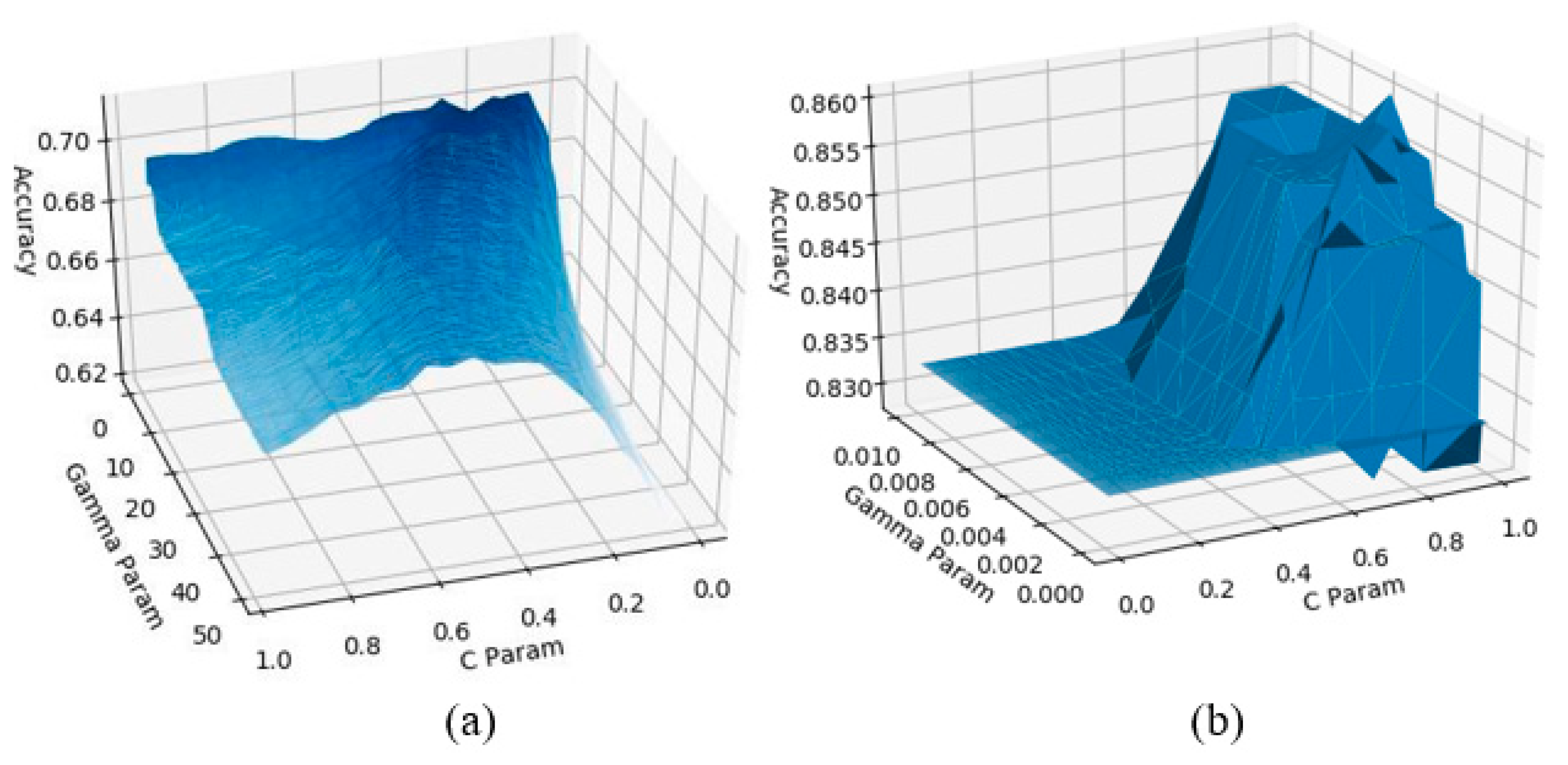
3.1.2. Support Vector Machine Modelling Process

Due to the high dimensionality and non-linear mapping ability, SVM is applied commonly as the ML model. The main working procedure of the SVM model for classification and regression can be found in [37,38] whereas the main theory behind the implementation of the model has been discussed in the S5 Section of the SI to shorten the article mainly. Generalizability is a key factor for the efficient SVR model.

In the study, radial basis function (RBF), defined as Equation (S8) in SI, was chosen as a kernel function in the SVM model where $x$ and $x^{\prime }$ represent the pairs of samples in training set, $\gamma$ is kernel coefficient to govern the effective value range of an individual training sample in a contrariwise relational design.

Support Vector Machine—Model Tuning

During training, overfitting may occur which can cause difficulty to predict new data accurately. Tuning can help to avoid this problem of overfitting. The regularization parameter $C$, mentioned in Equations (S5) and (S6) in the S5 Section of the SI, is another factor associated with the cost function of the SVM model. A higher $C$ value shows a low power in the model regularization technique while giving a higher accuracy for the training set but a greater difficulty in generalizing the testing set, known as overfitting. By contrast, lower values of $C$ can liberalize the accepting margin of decision function, resulting in lower training accuracy, recognized as underfitting effect. Hence, the generalization performance of the SVM model was also considerably impacted by the parameters $C$ and γ [39]. Grid search (GS) is an exhausted schema to run the experiments with all possible combinations of parameters. A five-fold cross validation was applied for the GS method of the SVM models. Here, the grid search algorithm was performed to choose the best possible pattern of $C$ and $\gamma$ for the classification model whereas GA was also utilized to determine the best combination of C and γ for the model. It had found that the best $C$ and $\gamma$ parameters were 0.853 and 0.003 for the SVM model.

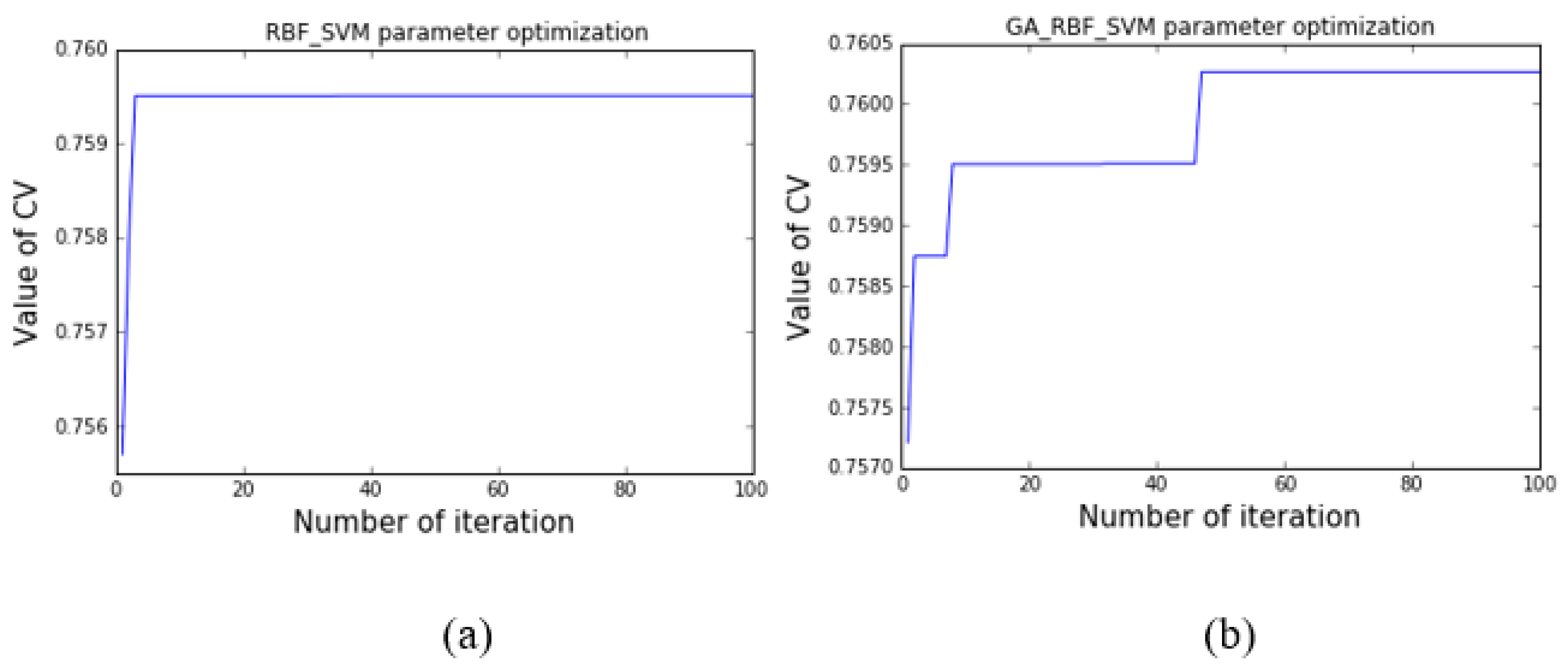
GA Supported SVM—Tuning Process

In this work, GAs have been used as a tool to boost the performance of ANN and SVM models. The two key hyperparameters optimized using the GA-supported SVM are C and γ. The model accuracy score function can use as the fitness function for the GA supported SVM modelling system. The detailed procedure of the SVM tuning process by GA has been mentioned broadly in the S6 Section of the SI Section. The pseudocode of the GA-supported SVM algorithm is presented in Algorithm 1. After we obtain the optimized C and γ, models are trained with the original features as inputs and the local correlation codes as outputs. Algorithm 1 table shows the overall GA-SVM model working procedures for the prediction of the crystal structure types and lattice parameters.

Algorithm 1: GA Supported SVM Modelling Algorithm

Data: ABO3 perovskite materials datasets $X\in R^{m\times n}$     Crystal Structure Label, $\mathrm{Y}\in R^{n\times L}$ (for SVM classification)  Lattice Parameters (a, b, c) Label, ${\mathrm{Y}}_R\in R^{n\times L}$ (for SVR regression) Output: Error function minimization Step 1: Initialize the SVM and GA parameters Step 2: Generate initial random population, Pi combining selected features and SVM parameters Step 3: Calculate the fitness evaluation function (accuracy score for 5 cross-validation of SVM) Step 4: Repeat Step 5:    Performing random Selection, Crossover, and Mutation Step 6:    Update population by evaluating the fitness function Step 7: Until satisfied the stopping criteria Step 8: Get the optimized C and γ for the SVM model and achieve the best accuracy for the model.

Like with the SVM model, an RBF kernel is also used for the GA-SVM model to predict crystal structures of the compounds. Figure 7 shows the hyperparameter optimisation for both the RBF-SVM model (Figure 7a) and the GA-RBF-SVM model (Figure 7b). These two hyperparameters have been determined using a GS with a five-fold cross validation. The accuracy of the GA-SVM is generally higher than for the SVM model. For the GA-SVM model, the maximum accuracy is found when C and γ are 1 and 8.1, respectively. The SVM model shows an optimal accuracy with relatively low C and γ parameters (Figure 7a).

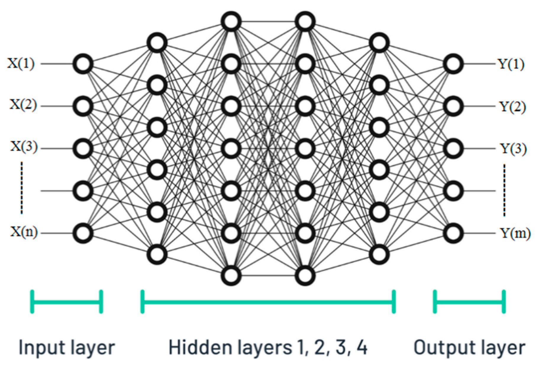
3.1.3. Neural Network—Modelling Process

A general neural network architecture used for our project has been shown in Figure 8. In this work, a multi-layer NN has been used to solve this non-linear problem. This provides a much better performance than the single-layer NN [40]. The performance constraints for assessing the ANN model are accepted as an error function, which is measured by loss function. The details of the NN modelling basic theory and standard processing techniques have been illustrated briefly in the S7 Section of the SI.

NN—Model Tuning

To obtain an efficient NN model, the following process parameters are varied: NN architectures; learning/training algorithms, and number of hidden neurons. In the NN model, inputs combined with the weight and bias matrix multiplication of sum are varied/renewed by applying some non-linear learning rule or training algorithm which can optimize the multi-variable of error function, which is called a minimization technique. For backpropagation, training algorithm Levenberg–Marquardt (LM) has been used for training the neural architectures. For the activation function, a sigmoid transfer function is used. All the important parameters for establishing the efficient NN model have been listed sequentially in the

Table 3. Significant Measurement of parameters for NN modeling.

Parameter	Data Range	Type of Technique Used
No. of input neuron	12
No. of hidden layers	4
No. of neurons in different hidden layer	6, 6, 6, 4
No. of output neuron	4
Total no. of sample	2225
Proportion of training and Cross-Validation datasets	80% & 20%
Data normalization	0 to 1	Min-max data normalization technique
Weight initialization	−0.5 to 0.5	Random weight initialization technique
Transfer function	0 to 1	ReLu function for hidden layers and SoftMax for output layer.
Error function		Loss function
Type of Learning rule		Supervised learning rule
Stopping criteria		Early stopping

.

A range of hidden layers has been tested to find out the best possible number of hidden layers to classify the ABO₃ crystal structure type. In this work, four hidden layers have been found effective throughout. The number of neurons in the input layer and the output layer are stable as the input parameters and label parameters. To investigate the effect of the number of neurons on model performance number of hidden neurons has been changed at different levels.

3.1.4. GA Optimized Neural Network (GA-NN) Modelling Process

GA is the computerized optimization technique built on the characteristics of natural genetics and natural selection. The purpose of the genetic algorithm studied in this work is to optimize the error function of the model for better performances from the modelling system where fitness function is derived from the objective function and used in the next genetic operations such as selection, reproduction, mutation, crossover, etc. operations. For the interested audience, the whole process of using GA as the optimizer for the ANN modelling system have explained deeply in the S8 Section of the SI.

Tuning Methods for the GA-NN Model

Due to the 2225 data samples of the current database, we have not used too many layers. Though more layers usually give better learning ability, it can cause overfitting as well. As such, four to six layers have been chosen with 4 to 15 nodes in each layer. For this model, we have selected four layers just like the simple NN modelling system, but we have taken different nodes for each layer than the simple ANN model. We have chosen 7, 6, 8, and 6 hidden neurons for the 1st, 2nd, 3rd, and 4th hidden layers, respectively. For this optimization, the conditions use as number of generations: 200; population size: 50; crossover rate: 0.8; mutation rate: 0.01; and mutation mechanism: multi-point. Algorithm 2 summarizes the GA optimized NN modelling algorithm for establishing an efficient model to predict the different crystal structures class.

Algorithm 2: GA Optimized NN Modelling Algorithm

Data: ABO3 perovskite materials datasets $X\in R^{m\times n}$     Crystal Structure Label, $\mathrm{Y}\in R^{n\times L}$ Output: Loss function optimization Step 1: Initialize the NN model objective function as fitness function Initialize the number of chromosomes, x; mutation rate, mu rate; and crossover rate value Step 2: Generate random population, P Calculate the fitness function f(x) of each chromosome x in the population Step 3: Repeat Step 4:    Update population by evaluating the objective function as fitness function Step 5:    Update after performing cross over with a crossover probability Pc Step 6:    Update with a mutation probability to mutate new offspring Step 7: Until satisfied the stopping criteria

3.2. Lattice Parameters Prediction Models

Lattice parameters can be useful in predicting material properties. As such, if the lattice parameters are not predicted well, it is impossible to define the other significant factors such as ionic or band gap. Therefore, there is a great interest in developing a method to correctly predict the crystal lattice parameter with a low sequential and computational cost. In this section, a successful lattice parameters prediction models have been introduced based on SVR and GA optimized SVR (GA-SVR) models.

The crystal lattice parameter depends on many atomic features including valence (z), ionic radius (r), and the electro-negativities (x) [24]. The prediction model of the lattice parameters has been developed in three parts: dataset composition; training process; and model evaluation. The first part involves dataset pre-processing, which is the same process as described in the classification modelling process previously. The second part and third part of the models are also considered with the same ratio of the datasets for the training and validation process. Two different regression models namely SVR and SVR-GA has been established to find out the best prediction models for the three lattice parameters of the crystal structure. These two models have the almost same construction process as the SVM and GA-SVM classification models.

3.2.1. SVR-Modeling Process

SVR is a regression algorithm which uses the same technique of SVM for the purpose of regression analysis. SVR can be used for working with continuous values instead of classification which is SVM. The regression datasets contain continuous real numbers. The SVR model has a particular margin called ε-tube (epsilon-tube, ε indicates a tube width) for fitting this kind of data, in regard to the model complexity and error rate. Here, kernel, C, γ and epsilon (ε) are important parameters, and they can be changed according to regression data characteristics. Different kernel function such as ‘rbf’ (default kernel), ‘linear’, ‘poly’, and ‘sigmoid’ can be utilized. As we discussed earlier, ‘rbf’ is used basically for the non-linear regression problems.

SVR-Model Tuning

Three models have been trained with the same initialized parameters except for the trade-off kernel parameters, C values to establish an efficient modelling system for the prediction of the lattice parameters. For the models of lattice parameters (a, b, and c), each model has been constructed using ‘RBF’ kernel function, ε-tube fixed with the value of 0.1, γ = 0.085, and the optimized C values for the a and b lattice parameters was 1.0 whereas 2.0 for the c lattice parameter prediction modelling system. Here, parameters have been optimized using the five-fold cross validation methods to evaluate the robustness of SVR-RBF model on predicting the label of testing samples [41].

In this work, from the 2225 datasets we have randomly chosen 80% of the datasets for the training purpose to build the successful model, whereas the remaining 20% have been used for the validation purpose. Due to the current comparatively small size of the database, the established SVR-RBF model was sensitive to various ratios of training and testing set. Hence, a five-fold cross-validation technique was iterated 200 times with different partitions of database to minimize the impact of imbalanced data distribution and consistently, 200 different SVR-RBF models were established. Later, the average and standard deviation value of evaluation criteria over 200 SVR-RBF models were calculated. After the establishment of the SVR modelling systems for the lattice parameters prediction, the model is needed to be verified using the cross-validation datasets. For the validation purpose, 20% of the whole datasets are randomly used to check the performance of the model through validation.

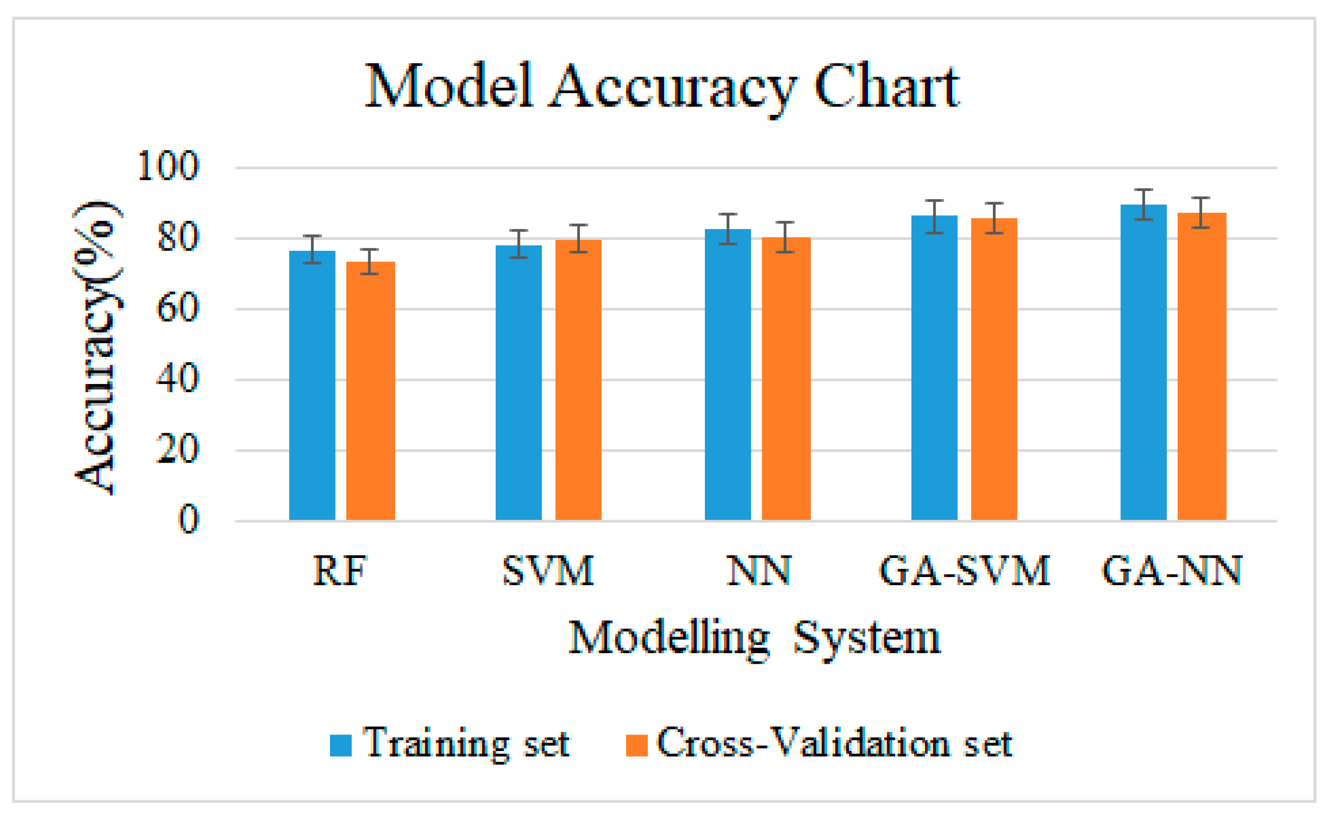
3.3. Model Accuracy

Performance evaluation is the important factor of a modeling to justify the efficiency of the model. Researchers using machine learning models express a model’s accuracy by using mean absolute error (MAE), root-mean-square error (RMSE), or coefficient of determination ($R^2$) [41]. However, these results explained the efficiency of those models by comparing their results with other ML modelling results and presenting the improvement in the performance of the ML modelling systems. Here, RMSE and $R^2$ were chosen as the evaluation criteria to quantify the accuracy of SVR-RBF models. The basic equation and standard way of determining the RMSE and R² have been discussed furthermore in the S9 Section of the SI.

4. Results and Discussion

The results section mainly focuses on the performances of the developed models for the classification of crystal structure and to predict the lattice constants of different crystal structures. From the performances of these models, we can see that SVR is very efficient not only to model a non-linear system but also SVM can successfully be able to classify non-linear datasets in such a way that the model provides a high rate of prediction accuracy. The NN model is familiar for the classification and regression modelling system, whereas we have found that it can outperform the classification job more accurately than SVM, RF, or GA-supported SVM. It gives the best prediction results classifying the crystal structures if GA can be added to the model for optimizing its tuning parameters.

4.1. Crystal Structures Prediction Models: Accuracy

Figure 9 shows the plot of the accuracy of the crystal structure prediction models. For each model, two accuracy values are presented: training set accuracy and validation set accuracy. The outcomes recorded here are applying the models that have been tuned to get the most excellent performance for the validation set.

All these results differ slightly for each time when the model is executed. This happens because of the random methods applied within the algorithms to make sure that the overfitting effect is never being caused. RF and NN have comparatively slight variations between each test. The accuracy of all these models has an error of about ±5%. All the data presented in the accuracy chart provides an average value and not a single test result.

The RF model provides the lowest accuracy of all the tested methods. The accuracy increases with the SVM, and this can be further enhanced by using the GA-optimized SVM model. A similar trend is also observed the NN. The NN accuracy is higher once again than the SVM accuracy. This accuracy is then further enhanced by using the GA-optimized NN. The best model performance is given by the GA-NN, which marginally outperforms the GA-SVM model.

The accuracy chart (Figure 9) shows that the performances of the different learning methods are different. Two different SVM settings illustrates a strong distinction between each other. At present, the GA-SVM model with C = 1 and γ = 8.1 is providing the top results compared to SVM model. From the figure, it can be seen that GA-optimized NN outperforms the GA-SVM model within a little difference as both models give higher accuracy for the prediction of the crystal structure types. From the chart, it can be seen that the GA-NN model shows the best prediction accuracy around ~88% compared to other modelling systems, which is quite high compared to the recent previous work [17] for such a large datasets.

4.1.1. Performance Comparisons for NN and GA-NN Models

The loss function optimizes the NN parameters and minimizes the NN loss by updating the weights, W_ji. For calculating the error of the NN classification model during the optimization process, a cross-validation function has been chosen as the loss function. To improve the NN model performance, the accuracy function was further optimized using a GA. GA was used as the accuracy function as the fitness function in the GA-NN model to optimize the model accuracy through the selection, crossover, and mutation GA operators.

Figure 10 shows the NN model and GA-NN model loss function as a function of epoch (iteration number). In this figure, the orange dots and the blue dots express the loss functions during the training period and the validation period, respectively. This figure shows that the NN model performs similarly in both the training and the validation sets. This proves that the model has a good generalizability. Finally, the GA-NN model has a better generalizability, compared to the NN model (Figure 10).

4.1.2. Performance Comparisons for SVM and GA-SVM Models

Figure 11a shows the cross-validation accuracy of the SVM modelling system for the RBF kernel without using GA optimization. Figure 11b shows the cross-validation accuracy of the GA-SVM modelling system for the RBF kernel using the GA optimization. From this figure, it is observed that the GA-SVM model achieves a higher accuracy compared to the SVM model during the cross-validation period. This proves that the GA has successfully optimized the C and γ parameters for the SVM model to improve the accuracy of the cross-validation performances.

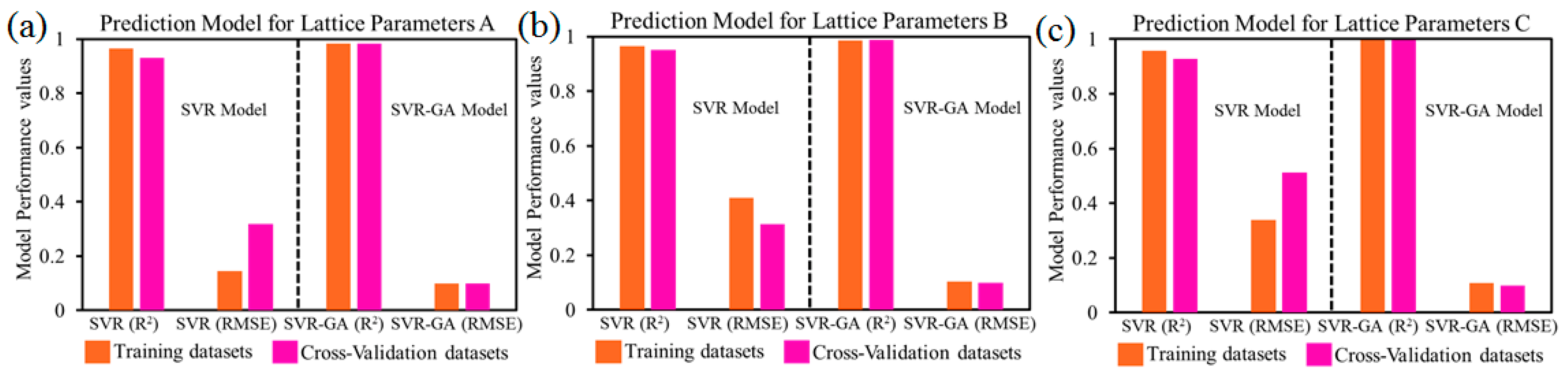
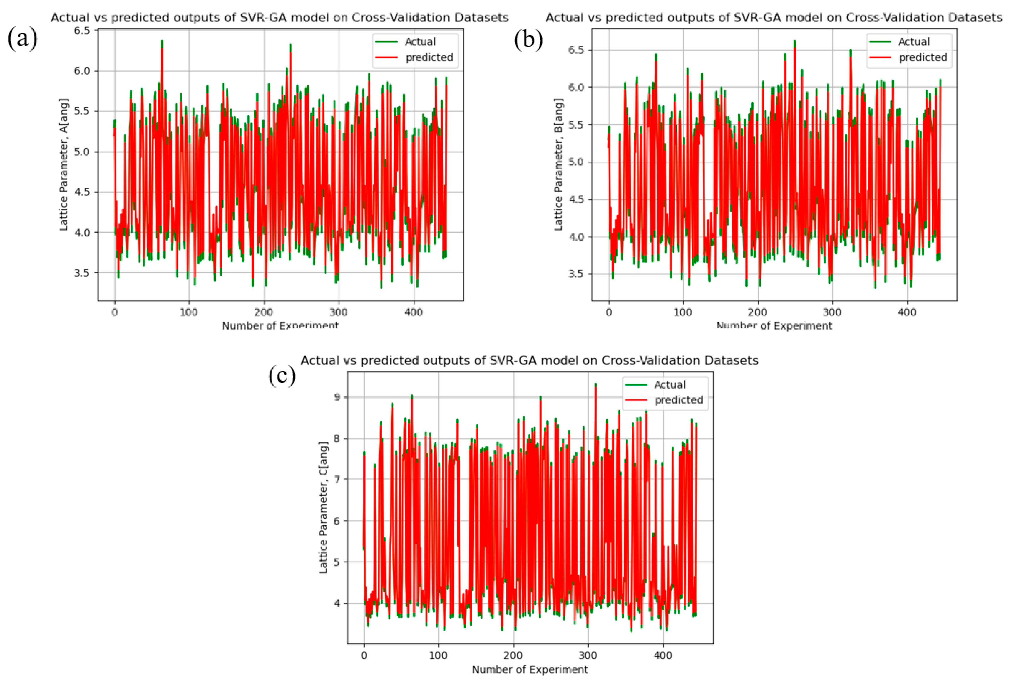
4.2. Lattice Parameters Prediction Models: Accuracy

Two ML models (SVR and GA supported SVR) have been used to predict three lattice parameters (a, b, and c) of ABO₃ type perovskite materials. Figure 12 shows the ML models performance values (R² and RMSE) for the training and the cross-validation datasets. The figure shows that these models have a high accuracy for the lattice parameter prediction. All three lattice parameters can be predicted with a similar accuracy using the SVR and the SVR-GA models. This proves that the models are well-trained for the prediction of lattice parameters. It can also be observed that the GA implementation improves the SVR modelling accuracy for each lattice parameter prediction. The SVR-GA model provides the best prediction model with an accuracy ~95% (±3) on average. This accuracy is high compared to the previous work [23,24] predicting the ABO₃ lattice parameters.

Figure 12a–c shows the performances of the SVR and SVR-GA models to predict the lattice parameter a, b, and c, respectively. From the figures, it can be seen that the SVR-GA model is well-trained as the accuracy for the training and cross-validation datasets is almost the same. In comparison, for the SVM model, the accuracy is not consistent for both the training and validation dataset. This suggests that the SVR-GA can be better trained in comparison to the SVR model.

Figure 13 shows the differences between the predicted and actual values of the lattice parameters. These figures also define the effectiveness of the SVR-GA modelling systems to predict the lattice parameters. From the figures, it is clear that most of the prediction is close to the actual values of those lattice parameters.

4.3. Models Performance Analysis: Discussion

It is necessary to analyze the performance of different models to know how good the model generalizability power is and find out the most efficient modelling system for the prediction of crystal structure and lattice parameters. The objective of these modelling systems is to develop a successful model so that this model can help researchers to save their time, cost, and labor for finding out new perovskite materials crystal structure along with its lattice constants. Another aspect of this work is also making the comparison of all these model’s efficiencies to predict the crystal structure types and lattice parameters of different ABO₃ materials.

Feature selection is the important part for these modelling systems, as efficient learning approaches highly depended on the selection of the optimal features. It is primarily needed for the modelling system to build a set of features that can describe the target variables accordingly and forward to reliable predictions. Therefore, we have selected features based on the importance factors got from the correlation Pearson’s co-efficient matrix. The features further extracted from the computational feature selection methods to eliminate the irreverent and redundant features. We have used RF algorithm also to confirm the effective features for all the models. Proper selection of relevant feature can help to reduce the dimensionality of the datasets. Thus, it can improve the generalization ability of the machine learning algorithms.

In this work, the model’s accuracy was measured for analyzing the performances of the model. The performances have been influenced by several factors, which can create the opportunity of further improvement for the modelling systems. For these modelling systems, the datasets of 2225 are being used, among which 1379 data samples are cubic, 651 data samples are orthorhombic, 131 data samples are rhombohedral, and 64 data samples are tetragonal. Therefore, it can be easily seen that these datasets are not well balanced where the number of samples for various classes have notable distinctions. These imbalanced datasets have an influence on the model algorithm. Though we have comparatively sufficient datasets in the database, the database contains few bad data or ‘noise’ as well. Hence, the accuracy for the imbalanced dataset will not be always as convincing as it is on some other datasets.

For random forest, however, it is a useful technique during the classification time; the classes with a small number of data samples have little impact to the classification process that could result a weak performance for the imbalanced datasets. SVM applies C for handling the accuracy of classification. Due to huge groupings of different number of layers, nodes, settings of the layer, and activation functions, it is difficult to tune the NN model perfectly. It is not easy to use the grid search method for an NN model because of the time-consuming nature of the NN model during the training period. The current problem is it is not yet a persuasive learning ability for the two tiny sample classes, which causes somewhat bad results as the accuracy for the validation set.

The differences between the models are clear due to the different tuning parameters for different modelling systems. Among the SVM models both the SVC and SVR models show that the high value of C has a better accuracy for both training and validation set. The grid search method usually yields the best consequence of hyperparameter selection, but the reality is that, yet a random selection of higher C can provide even a comparatively better performance because of the various evaluation characteristics. For tuning the other models, model accuracy for the validation set is considered for the valuation characteristics while GS can only provide the result based on cross validation. The effect for the cross validation would be distinct from the effect provided by a randomly selected validation set. Still, it needs further investigation on this issue. There is still some lack or deficiency in terms of model tuning and hyperparameters optimization process. This can create the hindrance to achieve better results than at present. Therefore, the models still have some pros and cons, which can be eliminated by using different optimization procedures such as partial swarm optimization (PSO) multivariate gradian descent etc.

The present work is mostly concentrated for the prediction of crystal structures and lattice parameters with the basic available atom characteristics. However, the attribute ‘valence’ is not an atom characteristic. This is deeply linked to the chemical structure. In this study, the valence feature defines which ionic radii is supposed to be used. The dataset’s impurity might have a little bit of an impact on the performance of the models. There are some faults in the current database, such as in some cases A site ionic radii is smaller than B site ionic radii, which is impractical. Other issues include A and B atoms having the same atomic element, which can impact the generalizability of the model.

The key points of this study are listed as follows:

(1) Implementing max-min normalization techniques on numerical features and label encoding on categorical features give the lowest prediction errors in the ML model.

(2) Basic atom characteristics have been used as the input features for the modelling system rather than providing any other structural or experimental information about the construction of the ABO₃ compounds.

(3) ML models can provide an accuracy of 88% around the classification class and ~95% for the regression model. This indicates that the ML models can be utilized for classifying the crystal structures successfully along with the efficient prediction of the lattice parameters.

(4) By applying the random forest (RF) algorithm, variable importance of each feature was evaluated, and a more concise database was then generated by eliminating the irrelevant features.

(5) GA can optimize the tuning parameters efficiently for the NN and SVM, which leads the GA-optimized NN and SVM model as the best performance model for the prediction of the crystal structures and lattice parameters of those crystal structures.

5. Conclusions

In this work, three basic ML algorithms are chosen. The objectives of these modelling systems are mainly two. One is to develop a successful model for the classification of different crystal structures, and the other is to use the same features and datasets to establish a mapping between the input and output parameters to predict the lattice parameters of these different crystal structures.

GA-NN model is found to be most suitable machine learning model for the prediction of the different crystal structure types with a higher accuracy of ~88% on average and better generalizability for this high-dimensional database. The SVR-GA model accuracy is ~95% (±3) on average, which shows the efficiency of the model for the prediction of the lattice parameters. The model accuracy is higher than other researchers have reported previously. These models, therefore, can be useful for the classification of the perovskite into their corresponding crystal structure types and lattice constants as a cost-effective, reliable, fast, and primary method, which could save time of the researchers from doing physical experiments or theoretical DFT calculation processes. Furthermore, the features’ importance findings and these developed models established an inference map between the basic atom characteristics and crystal structure type or lattice parameters from the ML models. These models could accelerate the design of new perovskite material with targeted properties for the renewable energy sources such as SOFC, PV panels, solar system, etc. As the different features have different impacts on the modelling system, we will focus on band gap, formation energy, etc. features in our future work to find out the effects of those features for the prediction of crystal structures and their corresponding lattice parameters.

References

- Guo, J.; Zhang, Y.; Lu, C. Effects of wetting and misfit strain on the pattern formation of heteroepitaxially grown thin films. Comput. Mater. Sci. 2008, 44, 174–179. [Google Scholar] [CrossRef]
- Khranovskyy, V.; Minikayev, R.; Trushkin, S.; Lashkarev, G.; Lazorenko, V.; Grossner, U.; Paszkowicz, W.; Suchocki, A.; Svensson, B.G.; Yakimova, R. Improvement of ZnO thin film properties by application of ZnO buffer layers. J. Cryst. Growth 2007, 308, 93–98. [Google Scholar] [CrossRef]
- Bouville, M.; Ahluwalia, R. Effect of lattice-mismatch-induced strains on coupled diffusive and displacive phase transformations. Phys. Rev. B 2007, 75, 054110. [Google Scholar] [CrossRef] [Green Version]
- Ashcroft, N.W.; Mermin, N.D. Solid State Physics; Ashcroft, N.W., Mermin, N.D., Eds.; Holt, Rinehart and Winston: New York, NY, USA, 1976. [Google Scholar]
- Terki, R.; Feraoun, H.; Bertrand, G.; Aourag, H. Full potential calculation of structural, elastic and electronic properties of BaZrO3 and SrZrO3. Phys. Status Solidi B 2005, 242, 1054–1062. [Google Scholar] [CrossRef]
- Li, C.; Soh, K.C.K.; Wu, P. Formability of ABO3 perovskites. J. Alloys Compd. 2004, 372, 40–48. [Google Scholar] [CrossRef]
- Cabuk, S.; Akkus, H.; Mamedov, A. Electronic and optical properties of KTaO3: Ab initio calculation. Phys. B Condens. Matter 2007, 394, 81–85. [Google Scholar] [CrossRef]
- Wang, H.; Wang, B.; Wang, R.; Li, Q. Ab initio study of structural and electronic properties of BiAlO3 and BiGaO3. Phys. B Condens. Matter 2007, 390, 96–100. [Google Scholar] [CrossRef]
- Wolfram, T.; Ellialtioglu, S. Electronic and Optical Properties of D-Band Perovskites; Cambridge University Press: Cambridge, UK, 2006. [Google Scholar]
- Galasso, F.S. Perovskites and High-T Sub c Superconductors; U.S. Department of Energy: Washington, DC, USA, 1990.
- Mizusaki, J. Nonstoichiometry, diffusion, and electrical properties of perovskite-type oxide electrode materials. Solid State Ion. 1992, 52, 79–91. [Google Scholar] [CrossRef]
- Glazer, A. Simple ways of determining perovskite structures. Acta Crystallogr. Sect. A Cryst. Phys. Diffr. Theor. Gen. Crystallogr. 1975, 31, 756–762. [Google Scholar] [CrossRef] [Green Version]
- Goldschmidt, V.M. Die gesetze der krystallochemie. Naturwissenschaften 1926, 14, 477–485. [Google Scholar] [CrossRef]
- Pradhan, S.; Moschitti, A.; Xue, N.; Ng, H.T.; Björkelund, A.; Uryupina, O.; Zhang, Y.; Zhong, Z. Towards robust linguistic analysis using ontonotes. In Proceedings of the Seventeenth Conference on Computational Natural Language Learning, Sofia, Bulgaria, 8–9 August 2013. [Google Scholar]
- Mitchell, R.H.; Welch, M.D.; Chakhmouradian, A.R. Nomenclature of the perovskite supergroup: A hierarchical system of classification based on crystal structure and composition. Mineral. Mag. 2017, 81, 411–461. [Google Scholar] [CrossRef] [Green Version]
- Hudspeth, J. Short-Range Order in Ferroelectric Triglycine Sulphate. Ph.D. Thesis, The Australian National University, Canberra, Australia, 2012. [Google Scholar] [CrossRef]
- Behara, S.; Poonawala, T.; Thomas, T. Crystal structure classification in ABO3 perovskites via machine learning. Comput. Mater. Sci. 2021, 188, 110191. [Google Scholar] [CrossRef]
- Podryabinkin, E.V.; Tikhonov, E.V.; Shapeev, A.V.; Oganov, A.R. Accelerating crystal structure prediction by machine-learning interatomic potentials with active learning. Phys. Rev. B 2019, 99, 064114. [Google Scholar] [CrossRef] [Green Version]
- Zhao, Y.; Cui, Y.; Xiong, Z.; Jin, J.; Liu, Z.; Dong, R.; Hu, J. Machine Learning-Based Prediction of Crystal Systems and Space Groups from Inorganic Materials Compositions. ACS Omega 2020, 5, 3596–3606. [Google Scholar] [CrossRef]
- Shandiz, M.A.; Gauvin, R. Application of machine learning methods for the prediction of crystal system of cathode materials in lithium-ion batteries. Comput. Mater. Sci. 2016, 117, 270–278. [Google Scholar] [CrossRef]
- Alade, I.O.; Olumegbon, I.A.; Bagudu, A. Lattice constant prediction of A2XY6 cubic crystals (A = K, Cs, Rb, TI.; X = tetravalent cation; Y = F, Cl, Br, I) using computational intelligence approach. J. Appl. Phys. 2020, 127, 015303. [Google Scholar] [CrossRef]
- Li, Y.; Yang, W.; Dong, R.; Hu, J. MLatticeABC: Generic lattice constant prediction of crystal materials using machine learning. ACS Omega 2021, 6, 11585–11594. [Google Scholar] [CrossRef]
- Javed, S.G.; Khan, A.; Majid, A.; Mirza, A.M.; Bashir, J. Lattice constant prediction of orthorhombic ABO3 perovskites using support vector machines. Comput. Mater. Sci. 2007, 39, 627–634. [Google Scholar] [CrossRef]
- Majid, A.; Khan, A.; Javed, G.; Mirza, A.M. Lattice constant prediction of cubic and monoclinic perovskites using neural networks and support vector regression. Comput. Mater. Sci. 2010, 50, 363–372. [Google Scholar] [CrossRef]
- Schütt, K.; Glawe, H.; Brockherde, F.; Sanna, A.; Müller, K.R.; Gross, E. How to represent crystal structures for machine learning: Towards fast prediction of electronic properties. Phys. Rev. B 2014, 89, 205118. [Google Scholar] [CrossRef] [Green Version]
- Iqtidar, A.; Khan, N.B.; Kashif-Ur-Rehman, S.; Javed, M.F.; Aslam, F.; Alyousef, R.; Alabduljabbar, H.; Mosavi, A. Prediction of Compressive Strength of Rice Husk Ash Concrete through Different Machine Learning Processes. Crystals 2021, 11, 352. [Google Scholar] [CrossRef]
- Aslam, F.; Elkotb, M.A.; Iqtidar, A.; Khan, M.A.; Javed, M.F.; Usanova, K.I.; Alamri, S.; Musarat, M.A. Compressive strength prediction of rice husk ash using multiphysics genetic expression programming. Ain Shams Eng. J. 2022, 13, 101593. [Google Scholar] [CrossRef]
- Kumar, A.; Verma, A.; Bhardwaj, S. Prediction of formability in perovskite-type oxides. Predict. Formability Perovskite-Type Oxides 2008, 1, 11–19. [Google Scholar]
- Oganov, A.R.; Glass, C.W. Crystal structure prediction using ab initio evolutionary techniques: Principles and applications. J. Chem. Phys. 2006, 124, 244704. [Google Scholar] [CrossRef] [Green Version]
- Pedregosa, F.; Varoquaux, G.; Gramfort, A.; Michel, V.; Thirion, B.; Grisel, O.; Blondel, M.; Prettenhofer, P.; Weiss, R.; Dubourg, V.; et al. Scikit-learn: Machine learning in Python. J. Mach. Learn. Res. 2011, 12, 2825–2830. [Google Scholar]
- McKinney, W. Data structures for statistical computing in python. In Proceedings of the 9th Python in Science Conference, Austin, TX, USA, 28 June–3 July 2010. [Google Scholar]
- Hunter, J.D. Matplotlib: A 2D graphics environment. Comput. Sci. Eng. 2007, 9, 90. [Google Scholar] [CrossRef]
- Emery, A.A.; Wolverton, C. High-throughput dft calculations of formation energy, stability and oxygen vacancy formation energy of ABO3 perovskites. Sci. Data 2017, 4, 170153. [Google Scholar] [CrossRef] [Green Version]
- Kantardzic, M. Data Mining: Concepts, Models, Methods, and Algorithms; John Wiley & Sons: Hoboken, NJ, USA, 2011. [Google Scholar]
- Sola, J.; Sevilla, J. Importance of input data normalization for the application of neural networks to complex industrial problems. IEEE Trans. Nucl. Sci. 1997, 44, 1464–1468. [Google Scholar] [CrossRef]
- Kotsiantis, S.; Kanellopoulos, D.; Pintelas, P.E. Data preprocessing for supervised leaning. Int. J. Comput. Sci. 2006, 1, 111–117. [Google Scholar]
- Smola, A.J.; Schölkopf, B. A tutorial on support vector regression. Stat. Comput. 2005, 14, 199–222. [Google Scholar] [CrossRef] [Green Version]
- Burges, C.J.C. A Tutorial on Support Vector Machines for Pattern Recognition. Data Min. Knowl. Discov. 1998, 2, 121–167. [Google Scholar] [CrossRef]
- Üstün, B.; Melssen, W.; Oudenhuijzen, M.; Buydens, L. Determination of optimal support vector regression parameters by genetic algorithms and simplex optimization. Anal. Chim. Acta 2005, 544, 292–305. [Google Scholar] [CrossRef]
- Jarin, S.; Saleh, T. Artificial neural network modelling and analysis of carbon nanopowder mixed micro wire electro discharge machining of gold coated doped silicon. Int. J. Mater. Eng. Innov. 2019, 10, 346–363. [Google Scholar] [CrossRef]
- Kohavi, R. A study of cross-validation and bootstrap for accuracy estimation and model selection. IJCAI 1995, 14, 1137–1145. [Google Scholar]