The Role of the Status-Quo in Dynamic Bargaining

Abstract

We analyze a dynamic bargaining game where parties can agree to implement a policy change, which is costly (beneficial) in the short-run but beneficial (costly) in the long-run. When the status-quo is endogenized (at least in some components), we show that the more farsighted party can induce their rival to accept the short-run costs of policy changes designed to generate benefits in the long-run. This is more common when players’ asymmetries are less pronounced, the status-quo is fully endogenized and the state depreciates more quickly.

1. Introduction

Negotiations often have a dynamic nature, from political parties who need to agree government budgets to countries negotiating over environmental issues. When agreements over such issues are reached, they are not everlasting, but revisited, as the state of the environment/economy/budget evolves over time (e.g., stock of CO₂ in the atmosphere/capital/government debt). The focus of this paper is on dynamic negotiations, where the agreements players reach today can affect future bargaining possibilities. By this, we mean two distinct dynamic features. On the one hand, we allow players the option of implementing costly actions, which may reduce current benefits, while also leading to higher future benefit (or vice-versa, they may increase short-run gain at the expenses of long-term benefits). With this, we aim to capture the feature in many dynamic negotiations that “investing” (in physical goods or goodwill, for instance) can have an impact on future bargaining possibilities. For instance, in COP26, 197 countries revisited the previous agreement (the Paris climate accord) and agreed to strengthen their current polluting emissions targets, a decision considered costly in the short-run but potentially life-saving in the long-run1. Conversely, by cutting the overseas aid budget the UK may have softened the government budget constraint in the short-run, but may also have weakened their diplomatic leverage in the longer term (according, for instance, to the Financial Times2). Undoubtedly, also the agreement the UK and EU reached after the Brexit referendum (and a long impasse) has affected, is affecting and will be affecting their relationship and their future bargaining possibilities for a long time3.

On the other hand, we allow an agreement (or at least some of its components), once struck, to become the status-quo, which serves as a threat point in future negotiations. Hence, in the case of an impasse/disagreement, negotiators implement the status-quo (the previous agreement in full or in part). The status-quo has been shown to be crucial for future negotiations in many examples, including trade deals for the UK, following Brexit4.

In this paper, we investigate a (two-player) bargaining game with two dynamic features of long-run negotiations: (1) apart from agreeing on how to split a surplus for their own consumption, players need to decide how much to invest (a higher investment today implies a lower current consumption but a higher surplus next period, and vice-versa); and (2) the status-quo is (potentially fully) endogenous. If players cannot strike an agreement, they implement (at least in part) the previous one (if any, or an initial status-quo).

We adopt the terminology in [1]—this is fully reviewed in the related literature below—which also endogenizes the status-quo, by investigating mandatory versus discretionary government spending programs in United States. Mandatory spending in the US government budget is expenditure driven by pre-existing law. Hence, it will be implemented in any spending bill, unless parties agree to change it. When all the spending components of the bill are mandatory, the status-quo is fully endogenized. Instead, discretionary spending will have to be negotiated at every spending bill. Hence, in case of disagreement, the spending for the discretionary components will be 0, even if players struck an agreement in the past. We use these definitions. Moreover, to fix ideas, in our model the players can be interpreted in two ways. First, they could be business partners who decide how to split a current profit, not only for their own consumption, but also on how to re-invest part of it, where investment affects the profit next period. The (initial) status-quo in this case is a (pre-bargaining) contract, specifying consumption and/or investment shares. The partners each period can either implement the contract or another split as long as they both agree to change the contract. Alternatively, the players are two political parties, as in [1], deciding on a budget and on whether or not to implement an existing policy (a split with mandatory/discretionary components)5. The key novelty in our paper is that their policy choice can affect the size of the surplus next period. The crucial question we aim to address is under which conditions parties implement changes in policy/contract?

To answer this question we investigate three types of status-quo: (1) the status-quo is fully endogenous, in other words all the components of the status-quo are mandatory; (2) only some components of the status-quo, for instance the consumption shares, are mandatory, while the remaining ones, investment in this case, are discretionary (even if players agreed to invest today, the status-quo for next period specifies 0 investment); and (3) differently from the previous two cases, where players can agree to implement any division (not just the status-quo), in this third case, to facilitate comparative statics, we consider the case in which some components of the status-quo are either not negotiable (these are unchangeable components, i.e., the cost of a potential change would be too high) or can only be increased (as the status-quo specifies only a minimum share).

We show that the status-quo persists, if Pareto efficient, otherwise, players agree to move to a Pareto superior division. With focus on the dynamics in a two-stage game, we shows that it is only one party who may benefit from the change. How much this player can gain depends not only on the consumption shares in the status-quo, but, crucially, also on how inefficient the status-quo investment is.

To further investigate the case of policy/contract changes, for the more complex case of asymmetric players, we consider the case in which the status-quo specifies only some components as mandatory (case 2 above). If only the consumption shares are mandatory, there is a tension between asymmetric players, as the more patient would ideally invest more than his rival (i.e., in a consumption-saving problem without bargaining his optimal investment would be higher). Hence, when bargaining, players make a compromise (unless they discount future payoffs strongly). The most impatient makes a concession by investing more than his ideal level, while the patient party makes a concession by reducing their current consumption to compensate their opponent and prioritize investment. An impatient opponent would be more willing to accept an offer with higher investment only if their current consumption is large enough.

However, if a party is sufficiently impatient, their ideal investment is 0. Hence, they can always exploit a status-quo, where investment is discretionary. When there are strong asymmetries, compromises do not arise in equilibrium, as impatient parties can always implement their ideal share of 0 investment. Only when the asymmetry between players is sufficiently low, are compromises possible, or otherwise it may be even possible for the most patient player to implement his (higher) ideal investment. This has implications for instance for costly policy changes. Populist political parties are often described as myopic (i.e., with a low discount factor). In this case, costly policy changes, with potentially long-term benefits, would never be implemented by these parties, but if less myopic, they may make compromises with more farsighted political rivals, which may give-up current consumption to compensate the myopic party. Indeed, if we compare the scenario with mandatory consumption shares with the one in which the consumption shares are instead unchangeable, compromises are less likely, as now the patient party cannot use the consumption channel to compensate the impatient player for investing.

Compromises are not an equilibrium phenomenon for the case of mandatory investment shares, even when the status-quo specifies a minimum investment. The key force is that responders have no bargaining power, when the status-quo prescribes no consumption and, therefore, the proposer can extract all the available surplus.

The analysis of the infinite-horizon game focuses on the steady-state. We show that any Pareto efficient consumption split can arise in equilibrium.

Related Literature—Bargaining theory has typically investigated negotiations characterized by only one of the dynamic features of our model: either the size of the surplus is fixed and the status-quo is endogenous or players can affect the size of the surplus but the status-quo is exogenous. A notable exception is [2], which considers a recursive bargaining game with endogenous status-quo. A crucial difference with our paper is that in [2] players can consume as much as they wish when they disagree, while in our framework they implement the previous agreement (/the initial status-quo), as in [1]. While [2] focuses on the tragedy of the commons (e.g., exploitation of natural resources), our focus is on the context of agreement changes in long-run negotiations. Also our analysis follows a fully non-cooperative approach.

Within the endogenous status-quo literature, the paper closest to ours is [1], which focuses on (mandatory versus discretionary) spending programs in United States, by investigating a bargaining game with a public good and private transfers, where two political parties bargain over a fixed government budget, under a take-it-or-leave-it offer. Medicare is as an example of mandatory spending, while military spending is an example of discretionary spending, as the latter has to be negotiated at every spending bill (see [1]). We adopt a similar framework but with two crucial differences. First, while in [1] the surplus is fixed in every period, in our framework, current policy choices (in particular, on how much to invest) will determine future surpluses6. This is relevant, as often major economic reforms (e.g., a more flexible labour market7) can be initially costly but could have long-term benefits (as it stimulates the economy and leads to higher future budgets). Second, in our model players may differ in terms of time preferences, while in [1], players are equally patient (but put different weights on the public good). The assumption of players with different time preferences is realistic and has been proven to enrich the analysis significantly (as shown, for instance, in the extensive review of bargaining theory in [4], in [5] in terms of agenda formation and [6] with focus on environmental issues).

The closest papers in dynamic bargaining are [4,7] (Section 10). The latter is the first contribution with a focus on a repeated (non-cooperative) bargaining game with investment decisions in addition to the standard consumption decisions. Since its focus is mainly on the steady-state of stationary subgame perfect equilibria [8], the investment decisions are simplified, as parties need to invest as much as necessary to have surpluses of the same size. Ref. [7] has the main aim of addressing the problem of how much parties invest in a strategic framework. In this paper, we adopt this framework with two (potentially heterogeneous) players who need to choose both how much to consume and how much to invest, but, in addition, we endogenize the status-quo. Hence, players can take actions in the current agreement which not only affect the size of future surpluses, but also set the threat point (or at least some of its components in future negotiations).

The paper is organized as follows. In the next section, we present the model. In Section 3, we solve it for the two-stage game. We focus on the case of symmetric players in Section 3.2. The case of asymmetric players and mandatory status-quo components is presented in Section 3.3. Section 4 covers the analysis of the infinite-horizon game. Section 5 concludes with some final remarks.

2. The Model

We consider a two-player bargaining game. Time is discrete and the horizon is potentially infinite, $t=0,1,\dots$ At each period, a surplus is generated according to the production function $F\left(k_t\right)=G{k}_t,$ where G is the constant gross rate of return and $k_t$ is the capital stock at period t. Once the surplus, $F\left(k_t\right)$, is generated the players, named 1 and 2, attempt to divide it. The status-quo at time t is a triple ${\mathbf{s}}_t=(s_{1t},s_{2t},{\phi }_{st})$ where ${\phi }_{st}$ is the status-quo investment share and $s_{it}$ is Player i’s consumption share over the remaining surplus with $s_{1t},s_{2t},{\phi }_{st}\in [0,1]$, $s_{1t}+s_{2t}⩽1$ and $i=1,2$.

At $t=0$, the status quo is given and named $\overline{s}=(\overline{x},\overline{y},\overline{\phi })$. The capital stock, $k_0,$ and the first surplus, $F\left(k_0\right)=G{k}_0$, are also given. The proposer at $t=0$ is randomly selected. Let p ($1-p,$ respectively) be the probability that Player 1 (2) makes the first offer. The bargaining procedure consists of a take-it-or-leave-it offer, in which players choose how much to invest and how to split the remaining surplus for their own consumption. Let ${\phi }_{it}$ be the investment share, Player i proposes at time t (with $i=1,2$), while $x_{1t}$ ($y_{2t}$) is the share of the remaining surplus Player 1 (2) asks to consume. Hence, an offer by 1 (2), at t, is the pair $o_{1t}=(x_{1t},{\phi }_{1t})$ ($o_{2t}=(y_{2t},{\phi }_{2t})$, respectively) with $x_{1t},y_{2t},{\phi }_{it}\in [0,1]$.

Consider an offer by, say Player 1, at time t, $o_{1t}.$ This can be either accepted or rejected. First, if it is accepted, the level of investment is $I({\phi }_{it},k_t)={\phi }_{1t}G{k}_t$ and the per-period consumption levels are

$$\begin{array}{ccc}\hfill c_1(o_{1t},k_t)& =& x_{1t}(1-{\phi }_{1t})G{k}_t\hfill \end{array}$$

(1)

$$\begin{array}{ccc}\hfill c_2(o_{1t},k_t)& =& (1-x_{1t})(1-{\phi }_{1t})G{k}_t\hfill \end{array}$$

(2)

The per-period utility has a logarithmic form8

$$u_i(o_{1t},k_t)=ln\left(c_i(o_{1t},k_t)\right)$$

(3)

with $i=1,2.$ Moreover, the output available at beginning of the next period, at $t+1,$ is $F\left(k_{t+1}\right)$, with capital stock $k_{t+1}$, given by the investment level, e.g., $I({\phi }_{it},k_t)$ and the capital remaining after depreciation $(1-\lambda )k_t$, where $\lambda$ is the depreciation rate ($0<\lambda \le 1$)9,

$$k_{t+1}=(1-\lambda +G{\phi }_{1t})k_t$$

Given the agreement, $o_{1t},$ at t, this becomes the status quo at $t+1$, $s_{t+1}=o_{1t}$ and will remain the status-quo in all subsequent periods $t^{\prime }$, with $t^{\prime }>t$, unless a new agreement is struck.

Second, if at t the offer $o_{1t}$ by Player 1 is rejected, the status quo ${\mathbf{s}}_t$ is implemented and at $t+1$ the state remains ${\mathbf{s}}_t.$ The capital stock is

$${\overline{k}}_{t+1}=(1-\lambda +G{\phi }_{st})k_t$$

Players alternate in making offers in each bargaining stage: the proposer at $t+1$, say j, is the player who responded to Player i’s proposal at t (regardless of whether or not this has been accepted) with $i,j=1,2$, $i\ne j$ and $t=1,2,\dots$.10 Player i’s discount factor is ${\delta }_i$.

We focus on Subgame Perfect equilibria (SPE) for the finite-horizon model and Markov Perfect Equilibria (MPE) for the infinite-horizon case. For the latter, the strategies specify players’ actions, for each time period $t,$ as a function of the state of the system at the beginning of that period. The state variables are the status-quo, $s_t$ (which is either the previous agreement, if any, or the initial status-quo, $\overline{s}$) and the capital stock, $k_t$.

Let $V_i({\mathbf{s}}_t,k_t)$ (respectively, $W_i({\mathbf{s}}_t,k_t))$ be the sum of discounted payoffs to Player i, when making an offer (responding to an offer) in an arbitrary MPE. Player i has to consider whether he is better off in making an acceptable offer, $o_{it}$, or implementing the status-quo, ${\mathbf{s}}_t$. Similarly, Player j will compare his payoff in case he accepts Player i’s offer $o_{it}$ or rejects it and therefore the status-quo ${\mathbf{s}}_t$ will be implemented. The problem can then be written in the following recursive form,

$$\begin{array}{ccc}\hfill V_i({\mathbf{s}}_t,k_t)& =& max\{V_i^{\prime }({\mathbf{s}}_t,k_t),ln\left(c_i(s_t,k_t)\right)+{\delta }_i{W}_i({\overline{\mathbf{s}}}_{t+1},{\overline{k}}_{t+1})\}\hfill \end{array}$$

(4)

$$\begin{array}{ccc}\hfill W_j({\mathbf{s}}_t,k_t)& =& max\{W_j^{\prime }({\mathbf{s}}_t,k_t),ln\left(c_j(s_t,k_t)\right)+{\delta }_j{V}_j({\overline{\mathbf{s}}}_{t+1},{\overline{k}}_{t+1})\}\hfill \end{array}$$

(5)

where $V_i^{\prime }({\mathbf{s}}_t,k_t)$ and $W_j^{\prime }({\mathbf{s}}_t,k_t)$ are the sums of discounted payoffs in case of an acceptance, while the second expression in brackets in (4) and (5) are the discounted payoffs in case of a rejection. Hence, for $i=1$

$$\begin{array}{c}{V}_1^{\prime }({\mathbf{s}}_t,k_t)=\underset{x_{1t},{\phi }_{1t}\in [0,1]}{\max }ln\left(x_{1t}(1-{\phi }_{1t})G{k}_t\right)+{\delta }_1{W}_1({\mathbf{s}}_{t+1},k_{t+1}))\end{array}$$

(6)

$$\begin{array}{c}\mathrm{s}.\mathrm{t}.W_2^{\prime }({\mathbf{s}}_t,k_t)\ge ln\left(s_{2t}(1-{\phi }_{st})G{k}_t\right)+{\delta }_2{V}_2({\overline{\mathbf{s}}}_{t+1},{\overline{k}}_{t+1})\end{array}$$

(7)

$$\begin{array}{c}{W}_2^{\prime }({\mathbf{s}}_t,k_t)\equiv ln\left(x_{2t}(1-{\phi }_{1t})G{k}_t\right)+{\delta }_2{V}_2({\mathbf{s}}_{t+1},k_{t+1})\end{array}$$

(8)

with the equations of motion given by

$$\begin{array}{ccc}& & \begin{array}{c}{k}_{t+1}=(1-\lambda +G{\phi }_{1t})k_t\mathrm{if}\mathrm{there}\mathrm{is}\mathrm{an}\mathrm{acceptance}\hfill \\ {\overline{k}}_{t+1}=(1-\lambda +G{\overline{\phi }}_t)k_t\mathrm{otherwise}\hfill \end{array}\hfill \end{array}$$

(9)

$$\begin{array}{ccc}& & \begin{array}{c}{\mathbf{s}}_{t+1}=(x_{1t},x_{2t},{\phi }_{1t})\mathrm{if}\mathrm{there}\mathrm{is}\mathrm{an}\mathrm{acceptance}\hfill \\ {\overline{\mathbf{s}}}_{t+1}={\mathbf{s}}_t\mathrm{otherwise}\hfill \end{array}\hfill \end{array}$$

(10)

Similarly, for $i=2$ (the subscript 1 and 2 are swapped and x is replaced by y, in (6)–(10). In the next section, we focus on a simplified model where there are only two periods. The infinite-horizon case is covered in Section 4.

3. A Two-Period Model

In this section, we assume that the game has only two periods. This allows us to show some key features of the game and its dynamics. First, in the following section, we show that the status-quo is preserved, whenever Pareto efficient. This is a result which will be shown to hold also in the infinite-horizon model and is in line with the existing literature (Bowen at al. (2014) [1]).

When players agree to change the status-quo, the randomly-chosen first mover can have an advantage. However, even for the two-period game, it is not straightforward to determine how exactly players agree to change the status-quo. Hence, in Section 3.2, the focus is on symmetric players. In this section, we derive the players’ equilibrium demands and quantify the first mover’s advantage. We will show that this depends not only on the status-quo consumption shares but also on how inefficient the status-quo investment share is. We then return to the case of asymmetric players in Section 3.3. In order to investigate further how players reach a compromise, we focus on the case in which only some elements of the previous agreement are mandatory.

3.1. Subgame Perfect Equilibrium

Since the game is finite, we use backward induction to identify the SPE. At the end of the game, any positive level of investment will be wasteful, hence, to avoid artificial inefficiencies, the status-quo at $t=1$ is set as ${\mathbf{s}}_1=(s_{11},s_{21},0)$. Hence, in case of disagreement, there is no investment, even if players have previously agreed a positive level of investment or the initial status-quo $\overline{s}$ prescribes a positive share (i.e., ${\phi }_{i0},\overline{\phi }>0$ at $t=0$)11. If Player 1 is the first mover at $t=1$, and this offer12 $o_1$ is accepted, then it must be

$$\begin{array}{c}(x_1,{\phi }_1)=\underset{x_1,{\phi }_1\in [0,1]}{argmax}ln\left(x_1(1-{\phi }_1)G{k}_1\right)\end{array}$$

(11)

$$\begin{array}{c}\mathrm{s}.\mathrm{t}.ln\left((1-x_1)(1-{\phi }_1)G{k}_1\right)\ge ln\left(s_{21}G{k}_1\right)\end{array}$$

(12)

Moreover, Player 1 must prefer $(x_1,{\phi }_1)$ to the status-quo,

$$max\{u_1(x_1,{\phi }_1,k_1),ln\left(s_{11}G{k}_1\right)\}=ln\left(x_1(1-{\phi }_1)G{k}_1\right)$$

It is intuitive that in the last period of the game, in equilibrium, there is no investment and the player making an offer leaves the opponent with the minimum consumption guaranteed by the status-quo and consumes the remaining surplus. This is formally shown next.

Proposition 1.

At $t=1,$ the SPE strategies are as follows: Player 1 proposes $(1-s_{21},0)$ and accepts any offer $o_2=(y_2,0)$ with $y_1=1-y_2⩾s_{11}$ and rejects it, if $y_1<s_{11}$ and/or ${\phi }_2>0$, while Player 2 proposes ($1-s_{11},0$) and accepts any offer $o_1=(x_1,0)$ with $x_2=1-x_1⩾s_{21}$ and rejects it, otherwise.

Proof. 

See Appendix A. □

Next, we solve the problem at $t=0.$ Given the initial status-quo, $\overline{s}=(\overline{x},\overline{y},\overline{\phi })$, if there is a rejection at this stage, players implement $\overline{s}$ and the sum of their discounted payoffs are

$${\overline{K}}_1=ln\left(\overline{x}(1-\overline{\phi })G{k}_0\right)+{\delta }_{1}ln\left(\overline{x}G{\overline{k}}_1\right)$$

(13)

$${\overline{K}}_2=ln\left(\overline{y}(1-\overline{\phi })G{k}_0\right)+{\delta }_{2}ln\left(\overline{y}G{\overline{k}}_1\right)$$

(14)

with ${\overline{k}}_1=(1-\lambda +G\overline{\phi })k_0$. Therefore, if Player 1 is chosen to make the first offer at $t=0$, the problem is

$$\begin{array}{c}{\varphi }_1=\underset{x_{10},{\phi }_{10}\in [0,1]}{\max ax}ln\left(x_{10}(1-{\phi }_{10})G{k}_0\right)+{\delta }_{1}ln\left(x_{10}(1-\lambda +G{\phi }_{10})G{k}_0\right)\\ s.t.ln\left((1-x_{10})(1-{\phi }_{10})G{k}_0\right)+{\delta }_{2}ln\left((1-x_{10})G{k}_1\right)\ge {\overline{K}}_2\end{array}$$

as long as Player 1 prefers to make an acceptable offer

$${\varphi }_1\ge {\overline{K}}_1$$

Similarly, for Player 2. Next, we show that it is subgame perfect to implement the status-quo, but only if Pareto efficient. Otherwise, the first player to make an offer will be able to improve his position by implementing a Pareto superior outcome, which leaves the opponent indifferent between accepting the offer and implementing the status-quo.

Proposition 2.

In equilibrium, players implement the initial status-quo ($\overline{x},\overline{y},\overline{\phi }$), if this is Pareto efficient, otherwise, they implement a Pareto efficient division where the first mover is always strictly better off, while the opponent’s payoff remains at the status-quo level.

Proof. 

See Appendix B. □

The ability of the first mover to extract all the remaining surplus is a feature of the two-stage game. More interestingly, Proposition 2 (and its proof) shows that although players will be able to implement a Pareto efficient outcome, ultimately it is not obvious to determine the features of the equilibrium (for instance, an interior solution is given by the solution of (A13) for the multiplier $m_1$, which is not obvious). We are interested in the following questions: will a policy/contract change be implemented and how? To address these questions, we first look at the simplified case of equally patient players.

3.2. Symmetric Players

For equally patient players (${\delta }_i=\delta$ for $i=1,2$), we can analytically derive the SPE strategies, hence, we can identify when players implement the status-quo, when they agree to change it and how they agree to change it. In the next proposition, we will show that the first mover has an advantage, summarized by a key factor, $f\left(\delta \right)$ in (16).

Proposition 3.

For ${\delta }_i=\delta ,$ with $i=1,2,$ players implement the status-quo division ($\overline{x},\overline{y},\overline{\phi }$) unless

$$(\overline{x}+\overline{y})f\left(\delta \right)⩽1$$

(15)

where

$$f\left(\delta \right)=\frac{(1+\delta )}{l}{\left[(1-\overline{\phi }){\left(\frac{1-\lambda +G\overline{\phi }}{\delta }\right)}^{\delta }G\right]}^{\frac{1}{(1+\delta )}}$$

(16)

with $l=G+1-\lambda .$ Under condition (15), in the SPE, players demand $x_1=1-f\left(\delta \right)\overline{y}$ and $y_2=1-f\left(\delta \right)\overline{x}$ and invest

$${\phi }_i={\phi }^{*}=\left\{\begin{array}{c}\frac{G\delta -(1-\lambda )}{G(1+\delta )}\mathit{for}G\delta >(1-\lambda )\\ 0\mathit{otherwise}\end{array}\right.$$

Proof. 

For ${\delta }_i=\delta$ for $i=1,2,$ FOCs (A8) and (A9) become

$$\begin{array}{ccc}\hfill x_{10}& =& \frac{1}{1+m_1}\hfill \\ \hfill {\phi }_{10}& =& {\phi }^{*}\hfill \end{array}$$

where for $m_1>0$, the indifference condition (A11) holds:

$$\begin{array}{c}(1+\delta )ln\left(\frac{m_1}{1+m_1}\right)+ln\left(\frac{l}{\left(1+\delta \right)G}\right)+\delta ln\left(\frac{\delta l}{1+\delta }\right)=\\ =(1+\delta )ln\overline{y}+ln(1-\overline{\phi })+\delta ln\left(\overline{\phi }\right)\end{array}$$

(17)

for $l=1-\lambda +G.$ Hence,

$$\frac{m_1}{1+m_1}=c_s$$

with

$$c_s=\overline{y}\frac{1+\delta }{l}{\left[(1-\overline{\phi })G{\left(\frac{1-\lambda +G\overline{\phi }}{\delta }\right)}^{\delta }\right]}^{\frac{1}{(1+\delta )}}$$

(18)

or $c_s=\overline{y}f\left(\delta \right)$, using the definition of $f\left(\delta \right)$ in (16). This implies $m_1=\frac{c_s}{1-c_s}.$ Therefore, the SPE demand is $x_{10}=1-c_s$ with $c_s<1$ for

$$\begin{array}{c}(1+\delta )ln\left(1-c_s\right)+ln\left(\frac{l}{G(1+\delta )}\right)+\delta ln\left(\frac{\delta l}{1+\delta }\right)⩾\\ (1+\delta )ln\overline{x}+ln(1-\overline{\phi })+\delta ln(1+\lambda +G\overline{\phi })\end{array}$$

(19)

where (19) ensures Player 1’s payoff when implementing $(x_{10},{\phi }_{10})$ is not smaller than the status-quo payoff ${\overline{K}}_1.$ Condition (19) can also be re-written as

$$c_s⩽1-\overline{x}f\left(\delta \right)$$

(20)

which together with $c_s=\overline{y}f\left(\delta \right)$, implies (15). □

The simple two-stage game highlights an important force. How much a proposer can gain depends on how inefficient the initial status-quo is. The smaller the sum $\overline{x}+\overline{y}$ is, the higher the share a first mover can extract. Moreover, as it is straightforward to show that $f\left(\delta \right)$ is maximized for $\overline{\phi }={\phi }^{*}$ and its maximum value is $f\left(\delta \right)=1$13, an implication of Proposition 3 is that the farther the status-quo investment $\overline{\phi }$ is from the efficient share ${\phi }^{*},$ the more the proposer can extract. Regardless of how unequal the status-quo consumption split is, as long as it is without waste, players will never agree to change it, if the investment share is efficient.

The factor $f\left(\delta \right)$, which summarizes how much more a proposer can extract, is affected also by the parameters of the model, $\lambda ,G,\delta$, apart from the status-quo investment share $\overline{\phi }$. The following corollary focuses on the case of infinitely-patient players and maximum depreciation.

Corollary 1.

For $\delta \to 1$ and $\lambda =1,$ players invest efficiently half of their surplus $({\phi }^{*}=1/2)$ and demand $x_1=1-f\left(1\right)\overline{y}$ and $y_2=1-f\left(1\right)\overline{x}$ with

$$f\left(1\right)=2\sqrt{(1-\overline{\phi })\overline{\phi }}⩽1$$

unless the status-quo is already efficient (i.e., $\overline{\phi }=1/2={\phi }^{*}$ and $\overline{x}+\overline{y}=1$).

Proof. 

For $\delta \to 1$, $f\left(\delta \right)$ in (16) tends to $2\sqrt{(1-\overline{\phi })\overline{\phi }}⩽1$, hence players change the status-quo, unless this is already efficient. If the status-quo is inefficient, following Proposition 3, players implement ${\phi }^{*}=1/2$ and the first mover’s demands are $x_1=1-f\left(1\right)\overline{y}$ and $y_2=1-f\left(1\right)\overline{x}$. If the status-quo is efficient ($\overline{\phi }=1/2={\phi }^{*}$ and $\overline{x}+\overline{y}=1)$, then $f\left(\delta \right)=1$, $c_s=\overline{y}$ (using (18)) and $x_1=1-\overline{y}=\overline{x}$ and $y_2=1-\overline{x}=\overline{y}$. □

Again, any change in the status-quo consumption will take place only if the split is wasteful and/or investment inefficient. In the two-stage game, a first mover can fully extract the potential gain of the change. Also in a longer horizon game, players will agree to implement an efficient split, however, we would expect that some concessions will take place in equilibrium.

In the next section, the focus is on asymmetric players and a partially endogenous status-quo (some components of the status-quo are mandatory, while the remaining, discretionary, components are set to 0 in any period).

3.3. Mandatory Components

In this section we investigate how asymmetry in players’ patience affects the solution. While in Section 3.1, we have shown that players agree to change the status-quo, if inefficient, in this section, we are interested in what outcome can arise when the starting status-quo is inefficient. For instance, the business partners may have signed a pre-bargaining contract, which makes only the consumption shares mandatory. Then the questions are: how will players invest? And how does this affect how they split the remaining surplus (as the mandatory shares are still negotiable)? Similarly, in the government budget in the United States, only some programs (e.g., Medicare) are mandatory. How will political parties agree on policies which may change the budget for the next period? Will this affect the mandatory spending?

The aim of this section is to identify the compromises parties can reach when only some components of the division are mandatory. We will show under which conditions, parties are more likely to agree to make costly investments to generate future beneficial gains.

In the next section, the focus is on mandatory consumption shares (while the status-quo investment share is set to zero in any period). We will show that the patient player may be able to negotiate an agreement with positive investment with a fairly impatient opponent, as long as the former can compensate the latter (by leaving the impatient player a larger consumption share). In Section 3.3.2, we will compare this with the case in which this compensation cannot take place, as the consumption shares are fixed (unchangeable). We will show that less flexibility can lead to fewer compromises, however, more investment will take place when the asymmetry is less pronounced. Section 3.3.3 concludes this part for the case of (minimum) mandatory investment share. Generally, for this case, we will show that players implement extreme consumption splits.

3.3.1. Mandatory Consumption Shares

In this section, we assume that in any period, the status-quo investment share is 0. Hence, the analysis follows closely the proof of Proposition 2, with the simplification that $\overline{\phi }=0$ (we had already set the status-quo investment share at the end of the game equal to 0). To identify how patience asymmetry (and the other parameters of the model) affect the solution, we look at numerical solutions and present a sample of cases below.

Let ${\varphi }_i$ (${\mu }_i$) be the equilibrium payoff, when Player i makes an offer $o_i$ (accepts his opponent’s offer $o_j$, respectively) at $t=0$14. Hence, for Player 1:

$$\begin{array}{ccc}\hfill {\varphi }_1& =& ln\left(x_1(1-{\phi }_1)G{k}_0\right)+{\delta }_{1}ln\left(x_1(1-\lambda +G{\phi }_1)G{k}_0\right)\hfill \\ \hfill {\mu }_1& =& ln\left((1-y_2)(1-{\phi }_2)G{k}_0\right)-{\delta }_{2}ln\left((1-y_2)(1-\lambda +G{\phi }_1)G{k}_0\right)\hfill \end{array}$$

Similarly, for Player 2.

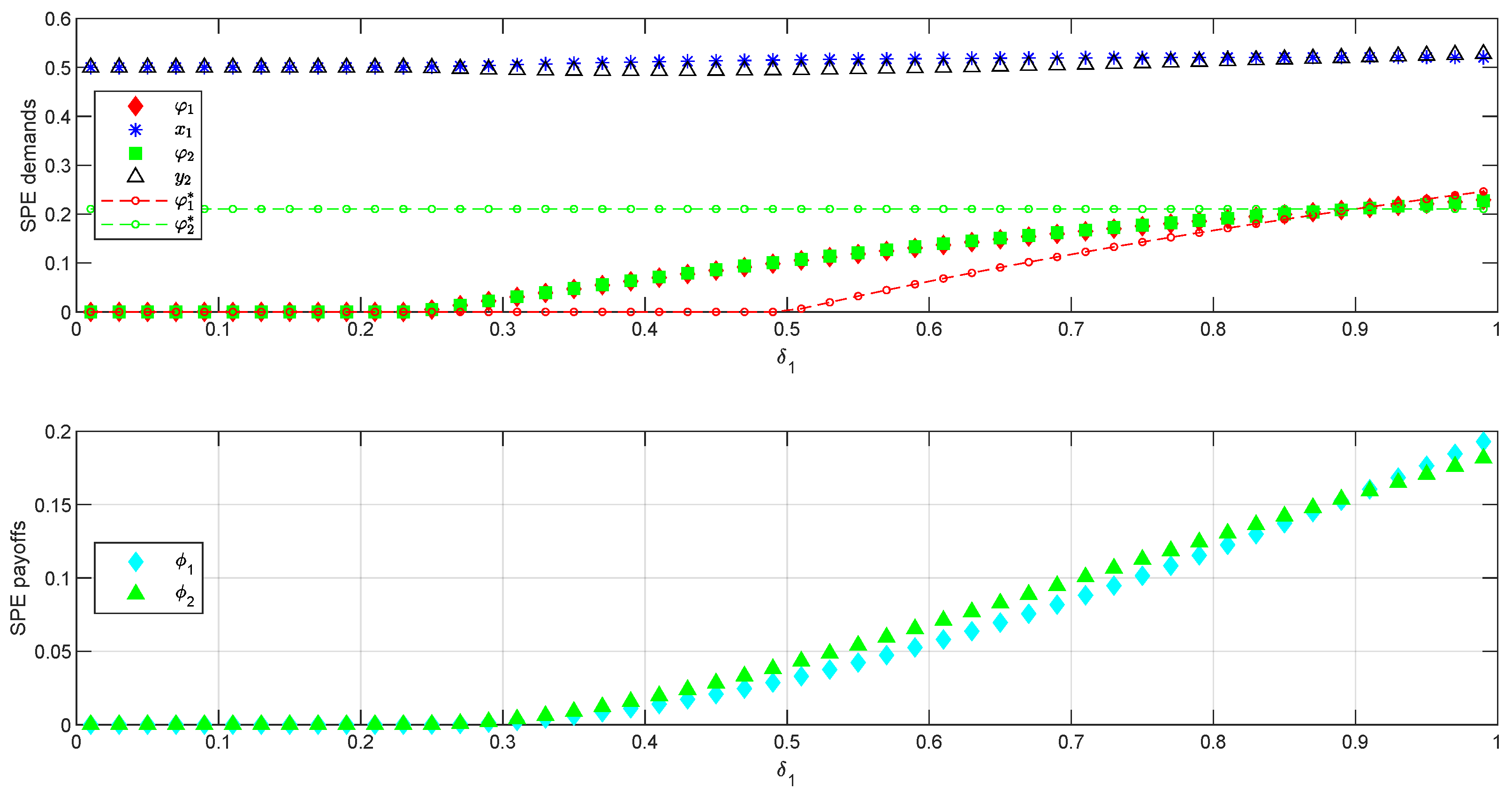
Figure 1 shows the effect of an increase in Player 1’s patience (${\delta }_1$, on the x-axis) on the SPE demands (first panel) and payoff coefficients (second panel) when the status-quo is $(0.5,0.5,0)$, ${\delta }_2=0.9$, $G=2,$ and $\lambda =0$15. In addition, the first panel shows the ideal investment shares (of the saving-consumption problem without bargaining):

$${\phi }_i^{*}=\left\{\begin{array}{c}\frac{G{\delta }_i-(1-\lambda )}{G(1+{\delta }_i)}\mathrm{for}G{\delta }_i>(1-\lambda )\\ 0\mathrm{otherwise}\end{array}\right.$$

with $i=1,2$. As indicated in the first panel of Figure 1, Player 2’s ideal share is constant, ${\phi }_2^{*}=0.21$, as it is unaffected by changes in Player 1’s patience. Instead, Player 1’s ideal investment share, ${\phi }_1^{*}$, is zero for ${\delta }_1⩽0.5$ and increasing for ${\delta }_1>0.5$. Moreover, as we would expect, the ideal investment share is higher for the most patient player (${\phi }_i^{*}>{\phi }_j^{*}$ for ${\delta }_i>{\delta }_j$, with $i,j=1,2$ and $i\ne j$).

When we introduce bargaining and Player 1 is sufficiently impatient, i.e., ${\delta }_1<0.25$, players cannot reach any compromise in equilibrium. As a result, they implement the status-quo, equally splitting the surplus without investing16. As ${\delta }_1$ increases (from ${\delta }_1⩾0.25$), Player 1 will start investing a positive share. This would be possible only for ${\delta }_1>0.5$ without bargaining. Hence, Player 1 is reaching a compromise with Player 2, who values investment more highly. While Player 1 invests an increasing share (for ${\delta }_1⩾0.25$), Player 1 is also able to extract a larger current consumption share. This is because he can exploit a trade-off between current and future consumption: by investing today, Player 1 has offered a larger surplus tomorrow and his patient opponent can accept to reduce his current consumption for a larger consumption next period. As shown in Figure 1, the consumption demands ($x_1,y_2$) remain relatively close to the status-quo value (0.5), however, Player 1’s demand, $x_1$, increases with ${\delta }_1$ (for ${\delta }_1⩽0.9$) while Player 2 initially sacrifices his consumption demand ($y_2$ decreases up to ${\delta }_1=0.43$). Only when players’ asymmetry becomes less pronounced, his consumption demand, $y_2,$ can increase. Indeed, when Player 1 is the most patient, ${\delta }_1>{\delta }_2=0.9$, he prioritizes investment (${\phi }_1>{\phi }_2$) and offers to consume a smaller share than Player 2 would, $x_1<y_2$. Interestingly, even with a strong asymmetry between players’ patience (and therefore a pronounced difference between their ideal investment shares, ${\phi }_i^{*}$), the more patient player invests only marginally more than the opponent (${\phi }_i>{\phi }_j$ for ${\delta }_i>{\delta }_j$ with $i,j=1,2$ and $i\ne j$), indicating the crucial role played by the status-quo: a more impatient player can always reject any offer with high investment. Only when equally patient (${\delta }_i=0.9$), will players invest their ideal share ${\phi }_2^{*}={\phi }_1^{*}$ (as indicated in Proposition 3).

The second panel in Figure 1 shows the SPE payoffs to the player making the offer (${\varphi }_i$), as Player 1 becomes more patient. The payoff when accepting an offer ${\mu }_i$, is omitted from the figure, as this remains equal to 0 (in this numerical example), the status-quo payoff, for any ${\delta }_1$. The increasing SPE investment shares are beneficial only to the player making the offer (both ${\varphi }_i$, with $i=1,2,$ increase). Indeed, the status-quo can be fully exploited by the first mover (in the two-stage game), as indicated in Proposition 2. Moreover, the increase in the payoff coefficient ${\varphi }_i$ is higher, for the more patient player.

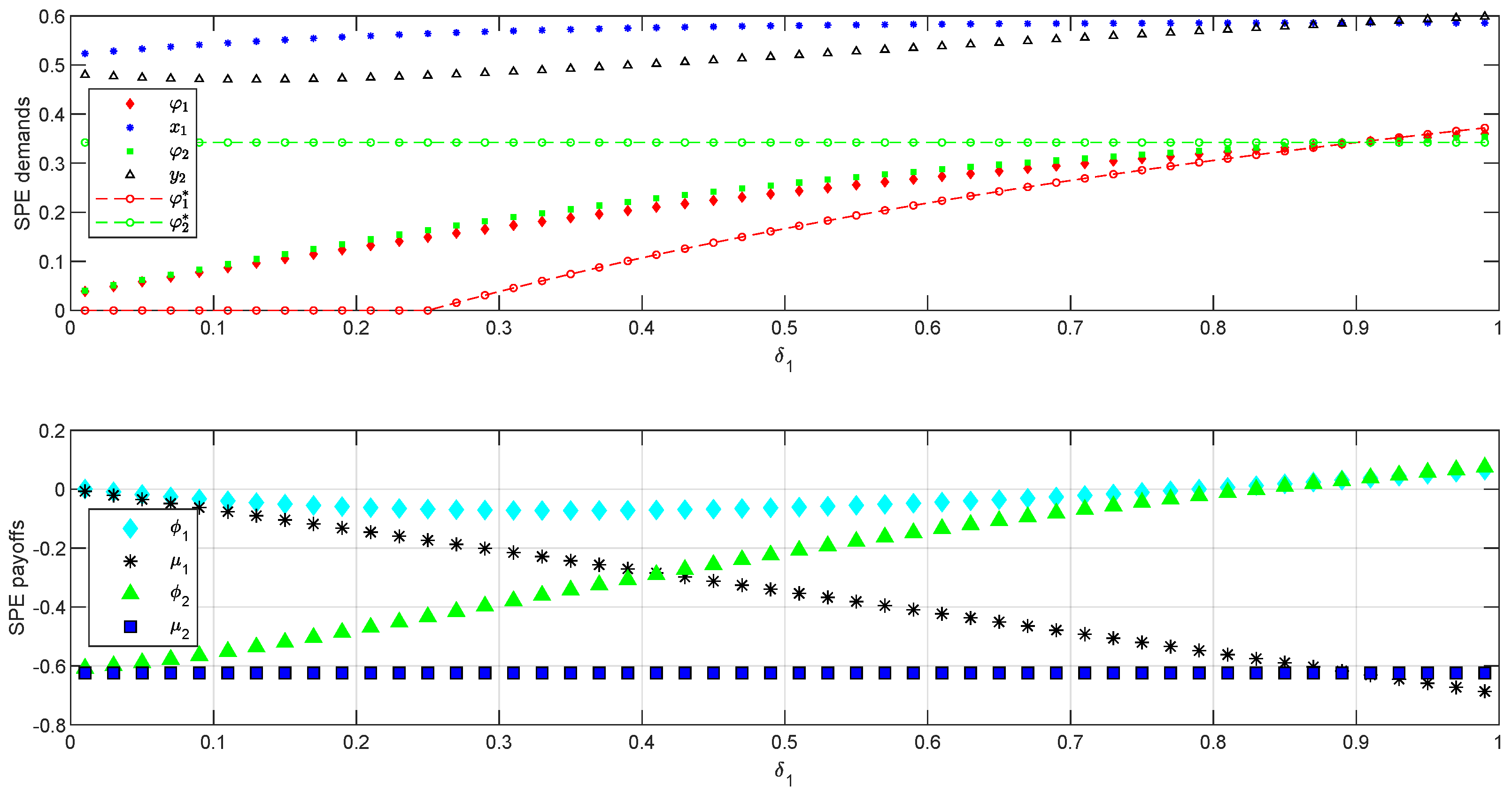
We next consider the case of a higher depreciation rate, $\lambda$. As this results in a smaller future surplus, we will show that players are more likely to make compromises and change the status-quo, ceteris paribus. As in Figure 1, Figure 2 shows the effect of an increase in Player 1’s patience (${\delta }_1$) on the SPE demands and ideal investment shares, ${\phi }_i^{*}$, (first panel) and payoff coefficients (second panel), for the same parameters as in the previous example (i.e., $(\overline{x},\overline{y},0)=(0.5,0.5,0)$, ${\delta }_2=0.9$, $G=2$), except for the depreciation rate, now positive, $\lambda =1/2$17. As in the previous example, Player 2’s ideal share is a constant (${\phi }_2^{*}=0.34$), while Player 1’s ideal investment is zero, when sufficiently impatient (${\delta }_1⩽0.25$) and increasing in ${\delta }_1$, otherwise. However, there is a crucial difference between the two numerical examples. Without bargaining, both players’ would invest more to compensate the higher capital depreciation. Indeed, ${\phi }_2^{*}$ is now a substantially higher constant (0.34, instead of 0.21) while Player 1 starts investing a positive share ${\phi }_1^{*}$ earlier (for ${\delta }_1>0.25$, rather than $0.5$). Both these elements push the relatively impatient player (1) to invest a positive share in equilibrium for any ${\delta }_1>0$. In turn, the higher investment share allows Player 1 to extract a larger consumption share, $x_1$, than in the previous example, again by exploiting the trade-off between current and future consumption.

The second panel in Figure 2 shows the SPE payoffs to the player making/accepting the offer (${\varphi }_i$/${\mu }_i$, respectively) as Player 1 becomes more patient. This shows that if Player 2 is the first mover, then he would be unambiguously better off with an increase in his opponent’s patience (${\varphi }_2$ increases with ${\delta }_1$). Player 2’s increased bargaining power is due to a weakening of Player 1’s status-quo (as ${\overline{K}}_1$ decreases with ${\delta }_1$)18. Instead, Player 2’s status-quo payoff is unaffected by changes in ${\delta }_1$ (similarly for ${\mu }_2$). Finally, if we allow for interpersonal comparisons, Figure 2 shows that the more patient player maintains the highest bargaining power, both as a proposer and as a responder (${\varphi }_i>{\varphi }_j$ and ${\mu }_i>{\mu }_j$, for ${\delta }_i>{\delta }_j$ with $i,j=1,2$ and $i\ne j)$, but given the (non-positive) effect on the status-quo, both players prefer to be first mover rather than responding to an offer (${\varphi }_i>{\mu }_i$ with $i=1,2)$.

The main conclusion of this analysis is that with mandatory consumption shares and asymmetry in players’ patience, the more patient/farsighted business partner will be able to make more substantial concessions (reducing his current consumption) to prioritize changes in investment. Similarly, for political parties, myopic/populist parties are less likely to take costly action to make policy changes. When the state depreciates faster (hence, the future surplus is smaller), even a very myopic party will take some actions to increase investment.

3.3.2. Unchangeable Consumption Shares

In the previous section, we have shown that players can agree to invest when there are asymmetries, as long as the patient player can compensate the impatient rival. In this section, we highlight the incentive to invest when the players cannot change the consumption share ($\overline{x}$ and $\overline{y}$ are fixed, with $\overline{x},\overline{y}>0$ and $\overline{x}+\overline{y}=1).$ We will show that in comparison to the previous section less flexibility may lead to less investment for a pronounced asymmetry. However, for weaker asymmetries, the more patient player will invest more than in the case of (negotiable) mandatory consumption shares.

The last stage is straightforward: since players do not invest and the consumption shares are exogenously given, they implement $(\overline{x},\overline{y},0).$ Let ${\phi }_{i,F}$ be the SPE investment share proposed by Player i at $t=0$, in the case of fixed consumption shares, with $i=1,2.$ Then, Player 1’s problem is

$$\begin{array}{c}\underset{{\phi }_{1,F}\in [0,1]}{\max }ln\left(\overline{x}(1-{\phi }_{1,F})G{k}_0\right)+{\delta }_{1}ln\left(\overline{x}G(1-\lambda +G{\phi }_{1,F})k_0\right)\end{array}$$

(21)

$$\begin{array}{c}ln\left(\overline{y}(1-{\phi }_{1,F})G{k}_0\right)+{\delta }_{2}ln\left(\overline{y}G(1-\lambda +G{\phi }_{1,F})k_0\right)\ge {\overline{K}}_2\end{array}$$

(22)

with ${\overline{K}}_2$ as in (14) with $\overline{\phi }=0:$

$${\overline{K}}_2=ln\left(\overline{y}G{k}_0\right)+{\delta }_{2}ln\left(\overline{y}G(1-\lambda )k_0\right)$$

The Lagrangian of problem (21)–(22) is

$$\begin{array}{ccc}& & ln\left(\overline{x}(1-{\phi }_{1,F})G{k}_0\right)+{\delta }_{1}ln\left(\overline{x}G(1-\lambda +G{\phi }_{1,F})k_0\right)+\hfill \\ & & -m_1\{{\overline{K}}_2-[ln\left(\overline{y}(1-{\phi }_{1,F})G{k}_0\right)+{\delta }_{2}ln\left(\overline{y}G(1-\lambda +G{\phi }_{1,F})k_0\right)]\}\hfill \end{array}$$

The FOC with respect to ${\phi }_{1,F}$ is as in (A6):

$$\frac{({\delta }_1+m_1{\delta }_2)G}{1-\lambda +G{\phi }_{1,F}}⩽\frac{1+m_1}{1-{\phi }_{1,F}};{\phi }_{1,F}\left(\frac{({\delta }_1+m_1{\delta }_2)G}{1-\lambda +G{\phi }_{1,F}}-\frac{1+m_1}{1-{\phi }_{1,F}}\right)=0$$

(23)

The analysis follows closely the proof of Proposition 2, however, an interior solution for ${\phi }_{1,F}$, as in (A9), now relies on the following indifferent condition:

$$ln(1-{\phi }_{1,F})+{\delta }_{2}ln(1-\lambda +G{\phi }_{1,F})={\delta }_{2}ln(1-\lambda )$$

or, using ${\phi }_{1,F}$ in (A9),

$$ln\left(\frac{l(1+m_1)}{G{f}_1\left(m_1\right)}\right)+{\delta }_{2}ln\left(\frac{l({\delta }_1+m_1{\delta }_2)}{f_1\left(m_1\right)}\right)={\delta }_{2}ln(1-\lambda )$$

(24)

with $\lambda <1$. A solution $m_1>0$ to (24) defines the optimal (interior) solution for the investment share in the case of unchangeable consumption share. As shown in the proof of Proposition 2, however, players may also be able to implement their ideal investment. The next example show more clearly when the status-quo is changed and how.

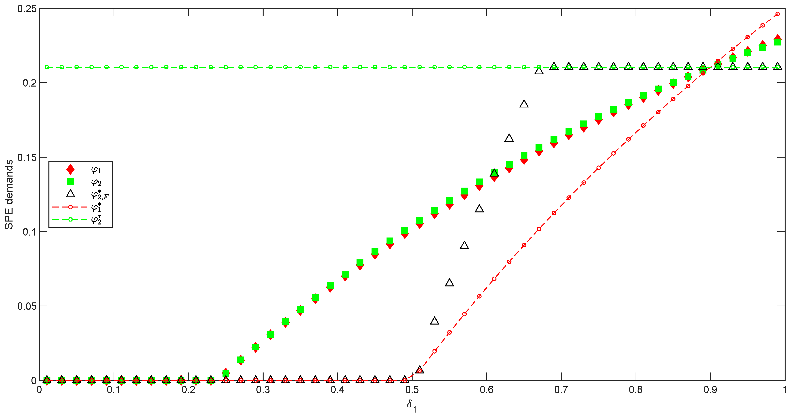
Figure 3 compares the SPE investment shares $({\phi }_1,{\phi }_2)$ in Figure 1, where players can agree to change the status-quo $\overline{s}=(0.5,0.5,0),$ with the case of unchangeable consumption shares (for the same parameter constellation, $G=2$, $\lambda =0$, ${\delta }_2=0.9$). In equilibrium, the relatively impatient Player 1 can always impose his ideal investment ${\phi }_{i,F}={\phi }_1^{*}$ (red dotted curve in Figure 3). However, Player 2 can do so (${\phi }_2^{*}=0.21$) only when the asymmetry in patience is less pronounced (${\delta }_1⩾17/25).$ To explain these results, consider first the case of ${\delta }_1⩽1/2$. In this case, Player 1’s ideal investment coincides with the status-quo, ${\phi }_1^{*}=0=\overline{\phi }$, hence Player 2 has no other option than to offer 0 investment, as Player 1 will always reject any other offer. If, instead, Player 1 is sufficiently patient (${\delta }_1⩾17/25$), both players have a positive ideal investment share, ${\phi }_i^{*}>0$, and they can implement it when making an offer, as the status-quo is by far an inferior alternative for the opponent. Interestingly, for a middle range of ${\delta }_1$ values ($1/2<{\delta }_1<17/25$), Player 1’s ideal investment becomes positive (${\phi }_1^{*}>0$), hence, Player 2 can push Player 1 to accept an increasing investment share, with ${\phi }_{2,F}>{\phi }_1^{*}>0$. As ${\delta }_1$ increases and ${\phi }_1^{*}$ increases, Player 2 can move closer to his ideal share ${\phi }_2^{*}$, which can be implemented earlier than in Figure 1 (for ${\delta }_1⩾17/25$ instead of ${\delta }_1=0.9)$. It is now Player 2 who uses the status-quo as a threat (as no investment becomes highly costly to Player 1 too).

Figure 3 shows that when the consumption shares are not negotiable, players are able to implement their ideal investment shares ${\phi }_i^{*}$ more often than in the case of mandatory shares. Player 1 can do so, for any ${\delta }_1$ and Player 2 for ${\delta }_1⩾17/25$, while with mandatory consumption shares, players must compromise most of the time (i.e., in Figure 1 or Figure 3, ${\phi }_1$, in red diamonds and ${\phi }_2$, in green squares, lie between the ideal shares ${\phi }_i^{*},$ with $i=1,2$, for any ${\delta }_1>0.25$). Also, the status-quo with $\overline{\phi }=0$, is implemented more often by both players, for ${\delta }_1⩽1/2$ (rather than only ${\delta }_1<0.25$ in Figure 1).

The analysis of this section has highlighted that less flexibility may be preferred by one player. This can be either the more patient, when he can threaten the relatively impatient rival with a status-quo costly enough that it will not be implemented in equilibrium or it can be a very impatient player when his ideal investment coincides with the status-quo. In the latter, the status-quo will be implemented in equilibrium. The trade-off between current and future consumption is no longer present: while, with negotiable shares, the more patient party could leave a larger consumption share to the opponent to compensate him for accepting greater investment, with fixed consumption shares, this channel is no longer present.

As a result, with a strong asymmetry, it is less likely, that a compromise can be reached when the status-quo consumption shares are fixed rather than mandatory, as the patient/farsighted party has fewer instruments to compensate their opponent. However, the farsighted player can successfully push for compromises, when the asymmetry in patience is less pronounced.

3.3.3. Minimum Mandatory Investment

In this final subsection, we consider the case of mandatory investment $\overline{\phi }>0.$ Moreover, we set $\overline{\phi }$ as the the minimum share, hence, player can only agree to increase it. With this constraint we attempt to capture dynamic negotiations characterized by costly incremental changes. For instance, in negotiations over environmental issues, typically all parties agree on the direction of the change (e.g., reduction of polluting emissions), however, given the high cost only gradual incremental changes are implemented every time. Similarly, in start-ups, business partners may grow their capital slowly, at least initially19.

The initial status-quo is $(0,0,\overline{\phi }).$ First, we consider the case in which all the components of the status-quo are mandatory. Hence, although the consumption shares are initially set to 0, players can agree to increase them and the agreement they strike becomes the status-quo next period. Second, we will discuss the case in which the consumption shares are discretionary (the status-quo consumption shares are always equal to 0, even if players agree to increase consumption in any period). A player making an offer will always exploit a status-quo which prescribes 0 consumption to the responder. However, the status-quo will affect the solution significantly20.

Next, we consider a mandatory status-quo $(0,0,\overline{\phi }),$ where all the components can be changed, with the caveat that $\overline{\phi }$ is the minimum investment share. The first mover faces an unconstrained optimization problem (as the opponent’s acceptance condition is not binding).

Proposition 4.

If the status-quo is endogenous, with a mandatory minimum investment share, $\overline{\phi }>0$, the first mover at t=0 behaves as a dictator: increases the investment share to his ideal level ${\phi }_i^{*},$ if ${\phi }_i^{*}>\overline{\phi }$, or keeps it at $\overline{\phi },$ if ${\phi }_i^{*}⩽\overline{\phi }$, and consumes all the residual surplus.

Proof. 

At $t=1$, in equilibrium, the proposer leaves the opponent with the minimum consumption share as defined by the status-quo and consumes the remaining surplus (as investment is set to 0 at the end of the game). Then, at $t=0$, as ${\overline{K}}_i=-\infty$ for $i=1,2$, the acceptance condition is not binding. The first mover can implement his ideal division $(1,{\phi }_i^{*})$ if ${\phi }_i^{*}⩽\overline{\phi }$ or $(1,\overline{\phi })$ otherwise. □

This result also extends to the case in which all the initial status-quo components are 0, $\overline{x}=\overline{y}=0=\overline{\phi }$21, or the game has a longer horizon.

Second, we consider the case in which the status-quo consumption shares are discretionary (i.e., they remain equal to 0, even if players have previously agreed to consume a positive amount). In this case, it is obvious that the proposers extract all the available surplus, however, differently from the previous case (in Proposition 4), a first mover has no incentive to invest, regardless of his level of patience. To see this, consider the last period, using Proposition 1, the proposer extracts all the surplus, as the rival’s status-quo consumption share is 0. Then, at the beginning of the game, the proposer’s ideal division would be $(1,0),$ to consume all the available surplus, as, given the alternating-offer procedure, only his rival would consume a positive share in the next stage. However, since the minimum mandatory investment share is $\overline{\phi }>0$, the proposer is constrained to invest $\overline{\phi }$ and consumes all the residual surplus. Therefore, in this case differently from the fully mandatory case in Proposition 4, both proposers can consume a positive share (but leave the opponent with 0 per-period consumption)22.

4. The Infinite-Horizon Case

In this section, we extend the analysis to the infinite-horizon case. Some of the features of the finite-horizon model can be re-established. In particular, players can move to a Pareto superior outcome, if the status-quo is inefficient, this is in line with Bowen et al. (2014).

To see this, consider the problem for the proposer is in (4)–(10). For $T=\infty$, the state variables are the status-quo, $s_t$ (which is either the latest agreement, if any, or the initial status-quo, $\overline{s}$), and the capital stock, $k_t$. If players agree to change the status-quo, then it must be that the proposer gains, see (4), and using (7), the responder is also (weakly) better off. Hence, the status-quo is implemented, if Pareto efficient, otherwise players can move to a Pareto superior outcome.

Next, we show that there is an indeterminacy of equilibria in terms of consumption divisions in the steady-state. Any Pareto efficient split $(x,1-x)$ can arise in equilibrium.

Proposition 5.

The steady-state MPE is to implement the division $(x,y,\lambda /G),$ with $x,y\in [0,1]$, and $x+y=1.$

Proof. 

See Appendix C. □

To understand this result, consider the investment $I=\phi F\left(k\right)$, first. This must be equals to the depreciated capital $\lambda k,$ in the steady-state $k_t=k$ for any t. With a linear production function, $F\left(k\right)=Gk$, the investment share is independent of the capital stock, as $\phi =\lambda /G$23. The investment and consumption problems are now fully disjoined. Since any division $(x,1-x)$ is Pareto efficient, these can all be part of the steady-state MPE.

The indeterminacy in the steady-state is fully driven by the assumption of a linear production function. On one hand, this assumption allows us to enrich part of the analysis, as, for instance, differently from the literature, we can consider varying degree of capital depreciation (see footnote 9). On the other hand, in the steady-state, the investment and consumption problems become fully disjoined.

Therefore, in this sense, the analysis of the dynamics is more insightful than the one related to the steady-state of our model. Of course, the two-stage game in our paper is the simplest set-up dealing with the joint problem of consumption and investment.

5. Concluding Remarks

We have investigated the role of the status-quo in a bargaining game where players can influence the size of the future surplus. We have shown that even in a simple two-period model, the status-quo plays a crucial role in determining the extent to which policy changes can be implemented. Another key determinant is the asymmetry in players’ patience. Compromises are more likely to take place if a farsighted/patient party can compensate a myopic one. Moreover, a depreciating state may encourage even myopic parties to take some steps towards policy reforms. For the infinite-horizon problem, although the steady-state investment is obvious, we obtain a multitude of possible outcomes in terms of consumption splits, including extreme ones where a party does not consume anything. Moreover, it remains open the issue of which dynamics can lead to a specific steady-state and therefore which mechanisms can encourage more equalitarian agreements.

Another interesting extension would be to relax the simplifying assumption of a linear production function and investigate richer steady-states where the consumption and investment problems remain intertwined.

Finally, we have considered three main types of status-quo, however, others may also be interesting to explore. For instance, whenever a party rejects an offer, all the available surplus may be invested automatically. This may create significantly different dynamics (as now a farsighted party may prefer the status-quo more often) and raises the issue of which status-quo is superior for society.

References

- Bowen, T.R.; Chen, Y.; Eraslan, H. Mandatory versus Discretionary Spending: The Status Quo Effect. Am. Econ. Rev. 2014, 104, 2941–2974. [Google Scholar] [CrossRef]
- Sorger, G. Recursive Nash Bargaining over a Productive Asset. J. Econ. Dyn. Control. 2006, 30, 2637–2659. [Google Scholar] [CrossRef]
- Hoffmann, E.B.; Malacrino, D.; Pistaferri, L. Labor Market Reforms and Earnings Dynamics: The Italian Case; IMF Working Paper WP/21/142; IMF: Washington, DC, USA, 2021. [Google Scholar]
- Muthoo, A. Bargaining Theory with Applications; Cambridge University Press: Cambridge, UK, 1999. [Google Scholar]
- Flamini, F. First Things First? The Agenda Selection Problem in Multi-issue Committees. J. Econ. Behav. Organ. 2007, 63, 138–157. [Google Scholar] [CrossRef]
- Fishman, R. Heterogeneous Patience, Bargaining Power and Investment in Future Public Goods. Environ. Resour. Econ. 2019, 73, 1101–1107. [Google Scholar] [CrossRef]
- Flamini, F. Divide and Invest: Bargaining in a Dynamic Framework. Homo Oeconomicus 2020, 37, 121–153. [Google Scholar] [CrossRef]
- Rubinstein, A. Perfect Equilibrium in a Bargaining Game. Econometrica 1982, 50, 97–109. [Google Scholar] [CrossRef]
- Ljungqvist, L.; Sargent, T. Recursive Macroeconomic Theory; MIT Press: Cambridge, MA, USA, 2000. [Google Scholar]
Figure 1.
MPE for , , and .
Figure 2.
Figure 3.
MPE with compulsory consumption shares for , , and .
Disclaimer/Publisher’s Note: The statements, opinions and data contained in all publications are solely those of the individual author(s) and contributor(s) and not of MDPI and/or the editor(s). MDPI and/or the editor(s) disclaim responsibility for any injury to people or property resulting from any ideas, methods, instructions or products referred to in the content. |
© 2023 by the author. Licensee MDPI, Basel, Switzerland. This article is an open access article distributed under the terms and conditions of the Creative Commons Attribution (CC BY) license (https://creativecommons.org/licenses/by/4.0/).
Share and Cite
MDPI and ACS Style
Flamini, F. The Role of the Status-Quo in Dynamic Bargaining. Games 2023, 14, 35. https://doi.org/10.3390/g14030035
AMA Style
Flamini F. The Role of the Status-Quo in Dynamic Bargaining. Games. 2023; 14(3):35. https://doi.org/10.3390/g14030035
Chicago/Turabian StyleFlamini, Francesca. 2023. "The Role of the Status-Quo in Dynamic Bargaining" Games 14, no. 3: 35. https://doi.org/10.3390/g14030035
Note that from the first issue of 2016, this journal uses article numbers instead of page numbers. See further details here.