

Measuring the Difficulties in Forming a Coalition Government

Department of Microeconomics, University Leipzig, 04109 Leipzig, Germany
Games 2023, 14(2), 32; https://doi.org/10.3390/g14020032
Submission received: 10 January 2023
/
Revised: 23 March 2023
/
Accepted: 29 March 2023
/
Published: 31 March 2023
(This article belongs to the Section Applied Game Theory)
Abstract
:Electoral thresholds in the context of parliamentary elections are an instrument for preventing the fragmentation of parliaments and facilitate the formation of a coalition government. However, the clauses also introduce distortions and modify the equality of electoral votes in an election. In order to decide to what extent these negative effects can be accepted, it is necessary to measure the difficulties in forming a coalition government and to quantify the effects of electoral thresholds on these difficulties. For this issue, we introduce a concept based on cooperative game theory which takes into account the distribution of seats in parliament and coalition statements of parties.
1. Introduction
An electoral threshold is a provision in a proportional representation system according to which parties with below a certain share of all votes are not taken into account in the allocation of mandates. The justification for these electoral thresholds is that they prevent the fragmentation of parliaments and facilitate the formation of a coalition government [1,2,3].
In Germany, an electoral threshold of 5% exists at the federal level and at the state level.1 For the reasons stated in the first paragraph, this threshold is compatible with the Constitution (German: Grundgesetz) in the view of the Federal Constitutional Court [4]. However, this compatibility does not have to be permanent, and circumstances must be taken into account. At the level of a European election, Germany also had a 5% electoral threshold (European Election Law). In a judgment on 9 November 2011, the Federal Constitutional Court ruled that this threshold is not compatible with the Constitution, because in the European Parliament, no coalition government is formed [5]. Subsequently, the legislature introduced a 3% electoral threshold. This threshold was again rejected by the Federal Constitutional Court [6]. The question of whether and at what level an electoral threshold is compatible with the Constitution is therefore a current problem. An objective measure of when it is more difficult to form a coalition government and how this measure can be used to check whether an electoral threshold is appropriate to the circumstances in parliament is still lacking.
To establish objective measures, cooperative game theory can be used to model party voting power in parliaments. Interestingly, the voting power of a party in a parliament does not necessarily correspond to only its share of votes. The distribution of votes among the other parties is also influential. For example, if party A has 40% of the votes in a parliament and the remaining votes are distributed among an infinite number of other parties, then the voting power of A is very high. However, if only one other party exists (with 60% of the votes), the intuitive assumption is that A’s voting power will be close to zero, since it will be defeated in all votes. To determine the voting power of a party based on the vote shares of all parties, cooperative game theory provides an analytical framework with weighted voting games and voting power indices. Another factor that influences the voting power of a party is its coalition statements. These statements announce preferred coalition partners and excluded coalition parties. The statements have two effects. The initial purpose is to raise the political profile of the party. More specifically, politicians want to increase the attractiveness of their party and influence voters’ behavior. After elections, the statements influence the bargaining strengths of the parties. For example, the exclusion of coalitions might reduce the bargaining power. Some new indices or values of cooperative game theory exist that could measure a party’s voting power in parliaments under consideration of the excluded coalitions. More specifically, Ref. [7] introduced and axiomatized the ECSh value (excluded coalitions’ value based on the Shapley [8] value). The ECSh value enhances the approaches developed by [9,10] to model player preference for cooperation with some other players. In [11], the value was used to analyze the distributions of power in German coalition governments that were possible with respect to the opinion polls prior to the 2013 federal election. Reference [12] gives some general results on the effects of excluding cooperation in games using the ECSh value. In our analysis, in addition, we applied the Holler version [13,14] of the ECSh value — the ECHo value.
Based on parties’ levels of voting power measured by the ECSh value and the ECHo value, we applied a measure for concentration — the Herfindahl–Hirschman index [15]—to calculate the concentration of voting power. Our interpretation is that if the concentration is low, we have a parliament in which forming a government or a majority tends to be more difficult.
We performed the following analyses in our approach. First, we considered some theoretical issues with the effect of electoral thresholds on the concentration measure. This was followed by three applications of the concentration measure. First, in a simulation study that randomized election results for five parties, we showed how the concentration of voting power changes on average in all simulations when the electoral threshold is increased step by step. In the following two applications, real election results and coalition statements were considered. The electoral thresholds were constant in both cases. These applications test how our proposed concentration measures would have behaved in a historical context and to what extent they are thus a meaningful measure of the possibility of coalition formation in parliaments. The first application involves the analysis of seat distributions in the parliament of the Weimar Republic between 1918 and 1932. The second application analyzed the distribution of seats in the German federal parliament between 1990 and 2021.
2. Basic Notation
2.1. Cooperative Game Theory
A TU (transferable utility) game is a pair , where is the non-empty and finite set of players. In our paper, the parties are players. The coalitional function v assigns every subset K of N a certain worth which reflects the economic abilities of K (i.e., such that The number of players in N is denoted by n or
A special case of a TU game are weighted voting games. In these games, a voting body is modeled. Parliaments are voting bodies. A primary task is to determine the characteristic function v. Every party has a voting weight representing the seats of the party.2 The coalition function v assigns the worth one (winning coalition) to a coalition if more than half of all seats are owned/governed by coalition K. Hence, v is given by:
A power index is an operator that assigns (unique) payoff vectors to all games (i.e., uniquely determines a payoff for every party in every TU game). The Shapley value is one power index. To calculate the parties’ Shapley payoffs, rank orders on N are used. The set of these orders is denoted by ; rank orders exist. The set of parties before i in rank order , together with party i, is called The Shapley payoff of a party i is [8]:
When applying this value to parliaments, the Shapley value is called the Shapley–Shubik index, and the payoff of party i is interpreted as the voting power of i [16].
Another power index was introduced by [13,14]. They utilized ideas from [17,18]. For calculating the Holler voting power, the set of minimum winning coalitions of is used.3 These coalitions are minimal, in that any party’s defection will reduce the worth of the coalition to zero. They are defined by: The voting power of party i is:
whereby measures the number of times a party i is a member of a minimum winning coalition. Since it is common in German parliaments to form coalition governments that are minimum winning coalitions, the Holler power index is an appropriate power index.
The Shapley index and the Holler index differ in two ways. First, voting power with respect to the Holler index considers only minimum winning coalitions. Second, the Holler index weights the marginal contributions of parties equally. Therefore, considering both indexes provides coverage for a variety of approaches to determining voting power and allows us to place our results on broader footing. A more detailed survey of power indices is presented in [20,21,22,23,24].
As mentioned in the Introduction, prior to elections, parties make coalition statements and exclude coalitions with certain parties. These statements prevent coalitions and are modeled below. The set of i’s excluded coalition partners is denoted by A party excludes only coalitions with single parties; i.e., if party A can cooperate with both party B and party C, it cannot exclude cooperation in a tripartite alliance ; The set of coalitions that are not allowed based on is called with If i does not cooperate with we have i.e., if a party i does not cooperate with j, j cannot cooperate with All inadmissible coalitions are denoted by Thus, the admissible coalitions in the game are A game with excluded coalitions is a tuple The primary idea of the EC value is that only admissible coalitions are considered [7]. When calculating the EC value based on the Shapley value, we have:4
In the case of we have ECSh = Sh The sum of the payoffs does not have to equal 1, unlike the Shapley value. This expresses the fact that coalition exclusions make it more difficult to find a majority. For example, if two parties, each with more than 25% but less than 50% of the seats in parliament, exclude any coalition with other parties, then the total EC payoffs will be zero.
Similarly, we obtain the Holler version of the EC value by modifying :
We obtain [11]:
In addition, for this value, the parties’ payoffs need not to sum up to Again, in the case of we have EC Similarly to our explanation of the value, this means that exclusion of coalitions with parties holding seats will lower the concentration of voting power (see next Section).
The payoffs of the two values can be interpreted as a priori voting power in parliaments without the existence of a governing coalition. Decreasing payoffs of the parties mean that their influence on voting results decreases. Due to coalition exclusions, it is possible that is no longer distributed to the parties. This can be interpreted as a difficulty in forming a governing coalition. The extreme case — or respectively — then means that it is no longer possible to form a coalition government.
2.2. Concentration of Voting Power
The idea of our article is that the concentration of the a priori voting power of parties in a parliament operationalizes the capacity of the parliament to act. Concretely, we use the Herfindahl–Hirschman index [15] to determine the concentration of voting power of political parties. If this is low, we have a parliament in which forming a government or a majority tends to be more difficult, and possibly, more parties are represented in a coalition government. In such cases, the electoral threshold can serve to reduce the number of parties in parliament and increase the concentration of voting power.
In other applications, the Herfindahl–Hirschman index is used, for example, in sales markets to determine market penetration. In [26], the Herfindahl–Hirschman index is used to determine the concentration of voting power of the owners of firms. The Herfindahl–Hirschman index has been applied to measure the political competition or the concentration of political power in parliaments based on the seats distribtution of parties in [27,28,29,30]. Maux [31] applied the Herfindahl–Hirschman index to measure the political power within a coalition government after an election.
In our approach, we determine the concentration of voting power in a parliament, as:
respectively
Corollary 1.
Iff there is a party with we have regardless of the excluded coalitions.
In these cases, finding a majority or forming a coalition government is most readily accomplished; we obtain for party i since only coalitions with i are winning coalitions.
Corollary 2.
Iff there are n parties with and for all we have
respectively:
In the case of , we have and
In this case, all parties are symmetric, and worth is distributed among all parties equally. Hence, we have for all
3. Case Studies
3.1. Simulation
With our simulation study, we aim to show the effect of electoral thresholds on the two concentration measures. The exclusion of coalition parties is not considered, since options for this are very diverse.5 To illustrate our simulation, we show two examples:6
Example 1.
We have five parties with voting results and The electoral threshold is in a first step ; hence, all five parties are in the parliament, and the distribution of seats corresponds to the voting result. The Shapley payoffs are and From this, we have Raising the threshold to means that party 1 is no longer represented in the parliament. The seats in parliament are distributed with respect to the voting result of the four bigger parties. With rounding, we obtain and For this seat distribution, we have , and Raising the threshold gives a lower concentration of voting power with respect to the Shapley version of concentration of voting power.
Example 2.
Five parties are involved with voting results and Again, the electoral threshold is in the first step ; hence, all five parties are in the parliament, and the distribution of seats corresponds to the voting results. The Shapley payoffs are and From this, we have . By raising the threshold to the distribution of seats is (with rounding) and For this seat distribution, we have , and Raising the threshold gives a higher concentration of voting power with respect to the Shapley version of the concentration of voting power.
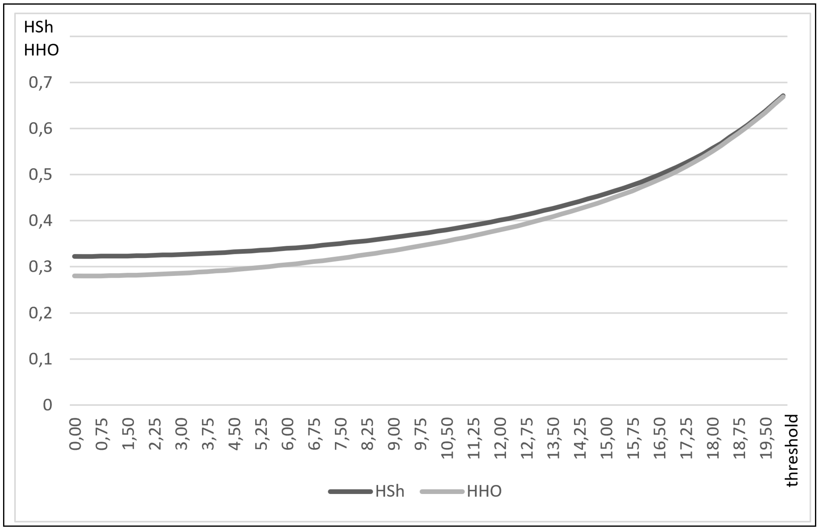
We simulated election results with five parties 100,000 times. For this, we have random votes assuming a uniform distribution of votes between 0 and 1 with For each voting result, we consider electoral thresholds between 0% and 20% in steps of 0.25. For each level of the electoral threshold, we determined which party is represented in parliament and calculate the share of votes in parliament for each party. From this, parties’ Shapley payoffs and Holler payoffs were computed. These were used to calculate the concentration measures and Figure 1 shows our average results for all simulations. Concentration with respect to the Holler index starts slightly below that of the Shapley one; both increase exponentially with the electoral threshold. Our results imply that the higher the electoral threshold, the stronger its impact on the concentration of voting power in parliament. Therefore, in our estimation, the legislature should carefully consider the level when introducing electoral thresholds and increase the requirements for consideration as the level of the threshold increases.
With respect to our examples, there is no case where an increase in the threshold results in a reduction of the concentration of voting power with respect to the Holler version of concentration of voting power. For the Shapley version, in 2.611 simulations, an increase in the threshold at some level reduces the concentration of voting power. Based on these results, the Holler version could be preferred for measuring the difficulties in forming a coalition government if an increase in the threshold should always lead to an increase in voting power concentration.
3.2. Weimar Republic Parliament: 1918–1932
In this section, we apply two concentration measures to the parliament of the Weimar Republic. We consider the seat distribution in parliament and the main excluded coalitions of the parties. As the proportion of parties uninterested in democratic cooperation increased over time, it is generally acknowledged that the difficulties of forming a coalition government increased. We aim to show that the two concentration measures reflect these increasing difficulties.
The electoral system of the Weimar Republic was a proportional representation system. In principle, a party received one seat in the Imperial Diet (German: Reichstag) for every 60,000 votes cast.7. An electoral threshold did not exist. Reforms of the electoral system were discussed throughout the existence of the Weimar Republic. One proposal was to increase the number of votes required per seat to 75,000. In addition, the aggregation of votes at the higher level was suggested to be capped. Other approaches included the introduction of elements of majority voting and electoral thresholds. The introduction of an electoral threshold would have increased the share of seats held by parties on the fringes of the party spectrum due to the high fragmentation of parties in the middle of the party spectrum. Therefore, this idea was rejected in the run-up to the 1930 election [32,33,34,35,36,37]. Decisions in the Imperial Diet were generally made by simple majority (exceptions existed, for example, for constitutional changes).
The entirety of excluded coalitions in the Weimar Republic is quite complex [38,39,40]. We concentrate on the main exclusions that demonstrate the application of our approach—i.e., we focus on the anti-republican parties on the left and right of the party spectrum, respectively, which were not seriously interested in parliamentary work. Concretely, we assume that the KPD (Communist Party of Germany) excluded all coalitions with other parties (with the exception of a possible cooperation with the USPD), and the NSDAP (National Socialist German Workers’ Party)8 excluded all possible coalitions.9 The results of our calculations are shown in Table 1. For the Shapley version of concentration of voting power, the results decrease from the election in 1920 to the election in May 1924. For the next two elections, the results increase a little bit. After this, the values decline, and starting from election in July 1932, the values are zero. Additionally, for , the highest value was calculated for 1920. Similarly to the Shapley version after this election, the concentration of voting power decreased for the election in May 1924 and increased for the election in December 1924. Differently to , the results decrease for 1928 and increase for 1930. Finally, both approaches reflect the fact that parliamentary majorities were no longer possible without the KPD and the NSDAP in both elections in 1932. Thus, our approach does well in modeling the problems of the Weimar Republic. The extent to which an electoral threshold would have alleviated the problems remains to be seen, since the parties were particularly fragmented at the center of the party spectrum.
To show the effect of coalitional exclusions, we computed a counterfactual scenario in which no coalitional exclusions existed. The results are shown in Table 2. The resulting concentration of voting power was higher than when coalition exclusions were taken into account. The strengthening of the anti-republican parties on the left and right of the party spectrum leads to an increase in the concentration of voting power in this calculation, since the fragmentation of the parliament decreases. Hence, not taking coalition exclusions into account would suggest that coalition formation was not affected toward the end of the Weimar Republic.
More fine-grained modeling of the preferences of parties in the Weimar Republic parliament was applied [41] for the 1919 election and the already undemocratic 1933 election. In their article, the parties are positioned on a spectrum and the values of the winning coalitions are weighted by the distances of the parties. After this, the Banzhaf–Penrose index [42] and intensity function values [43] are applied to them. In principle, the Shapley–Shubik index and the Holler index could also be applied to this weighted values of coalitions. The prerequisite to apply the approach by [41] is a detailed analysis of the positions and distances of the parties in the political spectrum of the Weimar Republic. Moreover, this method assumes that parties are positioned on a linear spectrum. However, cooperation between parties may be impossible despite the political proximity of them — e.g., if one party gets a splinter party (e.g., SPD and USPD during the German Empire, or SPD and WASG in 2004 in Germany).
3.3. German Federal Parliament: 1994–2021
In this final application, we analyze the German federal parliament from 1994 to 2021. Again, we consider the seat distribution in parliament and the main excluded coalitions of parties. As the number of parties in parliament has increased over the years and the AfD, a party with which the other parties do not want to form a coalition, has recently entered the parliament, the latest protracted negotiations to form a coalition government show that the difficulties of forming government have increased here as well. Again, we aim to show that the two concentration measures reflect these increasing difficulties. In addition, it is generally accepted that it was easier to form coalition governments in the period from 1994 to 2021 than at the end of the Weimar Republic — this should also be reflected in the concentration measures.
The election to the Bundestag (Federal Parliament) is regulated by law in the Federal Election Act (German: Bundeswahlgesetz). It is a personalized proportional representation election. Voters elect a direct candidate for their constituency with their so-called first vote. With the second vote, the state list of a party is elected. The distribution of seats in the Bundestag is based on the share of the second vote. If a party receives more direct candidates than the number of seats it is entitled to according to the two-vote share, these are allocated to it as overhang mandates. To compensate for the resulting shift in the proportions in the parliament, the other parties receive compensatory mandates.10 In § 6 (3) of the Federal Election Act, an electoral threshold of 5% is defined. Only parties whose share of the second vote is higher than this threshold are taken into account in the allocation of seats via the state lists. Alternatively, this quorum can be exceeded if a party receives three direct mandates.11 Detailed specifications for the 2021 election are described by [57], for example. The coalition statements for the parties are shown in Table 3. A historical overview and analysis of coalition statements of German parties are presented in [58,59,60,61,62]. Decisions in the Federal Parliament are generally made by simple majority (exceptions existed, for example, for constitutional changes).
The results of our calculations are shown in Table 4. The concentration of voting power for both concepts increased from 1994 to 2002. For 2005, both concepts produced their lowest values since 1994. For the elections in 2009 and 2013, the results increased. The last two elections in 2017 and 2021 resulted in low and low . This was due to the higher number of parties in the Bundestag and the existence of coalition exclusions from the parties. In particular, the rather high share of the AfD, combined with the coalition exclusion of the other parties, makes it more difficult to form a government and lowered the results for and . The first three-party coalition in government in 2021 was a result of this development. Compared to the Weimar Republic, however, the results (with limitations in 1920) are higher. This fits with the common opinion that coalition formation was much more difficult toward the end of the Weimar Republic than in the current situation in the German federal parliament. From this perspective, the results for and seem plausible according to both developments in the German Federal Parliament and compared to the Weimar Republic.
To show the effect of coalition exclusions, we also present an alternative calculation here. The exclusions are shown in Table 5. They are based on the traditional party alliances in the 1990s in Germany, in which a conservative bloc of CDU and FDP opposed the bloc of SPD and Grüne. A coalition with Linke was also ruled out by the SPD and the Grüne. Only the following developments in the last few years allow for fewer exclusions, as shown in Table 3 [63,64]:
- In Thuringia, starting in 2014, the SPD became the junior partner in a coalition government with Linke. In addition, there was the first coalition with SPD and Linke in a western state (Bremen) since 2019.
- CDU and Grüne govern together in Hesse (after elections in 2013 and 2018), Baden-Wuerttemberg (since 2016 the CDU is a junior partner), Saxony-Anhalt (since 2016), Schleswig-Holstein (since 2017), Brandenburg and Saxony (both since 2019). In Saxony and Saxony-Anhalt, cooperation between CDU and Grüne is necessary to form a coalition government.
- Grüne and FDP have been in a coalition government in Schleswig-Holstein (since 2017) and at the federal level since 2021.
As is to be expected, the concentration of voting power decreases as more excluded coalitions are taken into account (see results in Table 6). Hence, in this example as well, the two measures of voting power concentration model the situation appropriately.

Table 5.
Excluded coalition partners—German federal parliament.
| {Linke,AfD,Grüne} | {AfD,Linke,FDP} | {CDU,FDP,AfD,SPD,Grüne} | {SPD,Grüne,Linke} |
Table 6.
Results for German federal parliament in 1994–2021.
| 1994 | 1998 | 2002 | 2005 | 2009 | 2013 | 2017 | 2021 | |
|---|---|---|---|---|---|---|---|---|
| 0.015000 | 0.015000 | 0.015000 | 0.005000 | 0.015000 | 0.005000 | 0.002222 | 0.001111 | |
| 0.074074 | 0.074074 | 0.166667 | 0.005000 | 0.074074 | 0.024691 | 0.001543 | 0.002500 |
4. Conclusions
In this article, we presented an approach based on concepts of cooperative game theory that is able to measure the difficulties in forming a coalition government. Our simulation study and the application to two parliaments showed that the approach yields plausible results. In our simulation study with five parties, the concentration of voting power increases on average when the electoral threshold is increased step by step. For the Weimar Republic’s parliament, the two concentration measures reflect the generally acknowledged increase in the difficulty of forming a coalition government. The same result was obtained for the German federal parliament. In addition, the results for the concentration measures for the German federal parliament are higher than our results for the Weimar Republic parliament. This result fits in with the general assessment that forming a coalition government was more difficult in the Weimar Republic than in Germany between 1994 and 2021.
Electoral thresholds are enacted by the legislature and reviewed by courts to reduce these difficulties in forming coalitions. Thus, our approach can be one element to operationalize these difficulties and could be a tool for courts in reviewing electoral thresholds. Of course, the methodology presented should not be used for analysis alone and should be complemented by existing analyses. These analyses include demoscopic analyses, which provide statements on election results, and politological analyses, which examine excluded coalitions between parties. Another line of research could be a comparison of our approach to measure the difficulties in forming a coalition government with other measures used in the literature, such as the number of parties in a coalition government [65,66], the number of seats above majority quorum [67], the margin of victory [68,69] and the volatility of votes shares over time [70]. In addition, our approach could be applied for other analyses in which the difficulties of coalition formation or political competition in parliament are relevant, e.g., budget deficits [27,69,71,72,73,74], tax revenue [75], fiscal performance [30,76,77,78] and expenditure efficiency [29,79,80].
For further research, one objective could be an investigation of flexible electoral thresholds that are determined on the basis of objective criteria. It is conceivable that a certain concentration of voting power in parliament should be set as a target before the election and that this is achieved with a flexible threshold after the election, knowing the election results.12 This would allow electoral thresholds to be removed from the legislature as a political tool.
Methodologically, our analysis was limited, for example, with respect to the modeling of minority governments. In some countries, such as Denmark and Norway, it is common that a government does not have a majority of overall seats in the legislature. This situation could not be modeled satisfactorily with cooperative game theory. Another constraint in our model is that parties can only completely exclude cooperation. In reality, however, more complex constellations exist. Possibly, the approach of overlapping coalitions can be adapted here for better modeling [82]. Additionally, our model could be enhanced by considering situations in which parties make statements that they will not be a junior partner in a coalition government. To model this, decomposition of the n-person game using a matrix could be used [25,83]. In addition, voting power indices that take into account parties’ preferences on coalitions in a more detailed way [41,43] could be the basis for the Herfindahl–Hirschman index.
5. Data
Funding
This work was funded by the Open Access Publishing Fund of Leipzig University supported by the German Research Foundation within the program Open Access Publication Funding.
Data Availability Statement
The datasets analyzed during the current study are available from the corresponding author on reasonable request.
Acknowledgments
I am grateful to three anonymous referees for helpful comments on this paper.
Conflicts of Interest
The author declares no conflict of interest.
Code Availability
The code is available from the corresponding author on reasonable request.
| 1 | An overview of blocking clauses in other countries is given by [2]. |
| 2 | As is common in the academic literature, we assume that each party votes en bloc in the parliament. |
| 3 | Riker [19] shows in his book that the smallest minimum winning coalition will be formed. |
| 4 | In the interpretation of [25], excluding cooperation between i and j reduces the value of party i to party j to zero. |
| 5 | In applications of the following sections involving the Weimar Republic from 1918 to 1932 and the German federal parliament from 1994 to 2021, excluded coalitions are considered. |
| 6 | Given voting shares of a party i in an election with and , and electoral threshold b with and we have:
|
| 7 | For this purpose, the Weimar Republic was divided into 35 constituencies. Each party at constituency level received one seat in parliament for every 60,000 votes cast. Residual votes from these constituencies were transferred to the next evaluation level (constituency associations) and assigned to parties there. If a party received at least 30,000 votes at the constituency level, it could receive a seat in the parliament for 60,000 residual votes here. Finally, residual votes were transferred to the imperial election. Each party received one seat for every 60,000 votes remaining. A small party had an advantage if its supporters lived in regional concentrations |
| 8 | The same held for the NSFP (National Socialist Freedom Party) that existed in 1924 during the aftermath of the Beer Hall Putsch. |
| 9 | This restriction is controversial, as the NSDAP eventually entered into a coalition with the DNVP in 1933. |
| 10 | |
| 11 | Independently of this, each direct candidate of a constituency enters the Bundestag. |
| 12 | Analogously, [81] introduced variable qualified majority rules for decisions on shareholders’ meetings. |
References
- Antoni, M. Grundgesetz und Sperrklausel: 30 Jahre 5%-Quorum—Lehre aus Weimar? Z. Parlam. 1980, 11, 93–109. [Google Scholar]
- Krumm, T. Wie wirksam sperren Sperrklauseln? Die Auswirkung von Prozenthürden auf die Parteienzahl im Bundestag und im internationalen Vergleich. Z. Polit. 2013, 23, 393–424. [Google Scholar] [CrossRef]
- Decker, F. Ist die Fünf-Prozent-Sperrklausel noch zeitgemäß? Verfassungsrechtliche und -politische Argumente für die Einführung einer Ersatzstimme bei Landtags- und Bundestagswahlen. Z. Parlam. 2016, 47, 460–471. [Google Scholar] [CrossRef]
- Bundesverfassungsgericht. BVerfGE 82. 1990. Available online: http://www.servat.unibe.ch/dfr/bv082322.html (accessed on 20 March 2023).
- Bundesverfassungsgericht. 2 BvC 4/10. 2011. Available online: https://www.bundesverfassungsgericht.de/SharedDocs/Entscheidungen/DE/2011/11/cs20111109_2bvc000410.html (accessed on 20 March 2023).
- Bundesverfassungsgericht. 2 BvE 2/13. 2014. Available online: https://www.bundesverfassungsgericht.de/SharedDocs/Entscheidungen/EN/2014/02/es20140226_2bve000213en.html (accessed on 20 March 2023).
- Hiller, T. Excluded coalitions and the distribution of power in parliaments. Appl. Econ. 2016, 48, 321–330. [Google Scholar] [CrossRef]
- Shapley, L.S. A Value for N-Person Games. In Contributions to the Theory of Games; Kuhn, H.W., Tucker, A.W., Eds.; Princeton University Press: Princeton, NJ, USA, 1953; Volume 2, pp. 307–317. [Google Scholar]
- Myerson, R.B. Graphs and Cooperation in Games. Math. Oper. Res. 1977, 2, 225–229. [Google Scholar] [CrossRef] [Green Version]
- Alvarez-Mozos, M.; Hellman, Z.; Winter, E. Spectrum value for coalitional games. Games Econ. Behav. 2013, 82, 132–142. [Google Scholar] [CrossRef] [Green Version]
- Hiller, T. Excluded coalitions and the 2013 German federal election. Appl. Econ. Lett. 2018, 25, 936–940. [Google Scholar] [CrossRef]
- Hiller, T. The effects of excluding coalitions. Games 2018, 9, 1. [Google Scholar] [CrossRef] [Green Version]
- Holler, M.J. Forming Coalitions and Measuring Voting Power. Political Stud. 1982, 30, 262–271. [Google Scholar] [CrossRef]
- Holler, M.J.; Packel, E.W. Power, Luck and the Right Index. J. Econ. 1983, 43, 21–29. [Google Scholar] [CrossRef]
- Hirschman, A.O. The Paternity of an Index. Am. Econ. Rev. 1964, 54, 761–762. [Google Scholar]
- Shapley, L.S.; Shubik, M. A Method for Evaluating the Distribution of Power in a Committee System. Am. Political Sci. Rev. 1954, 48, 787–792. [Google Scholar] [CrossRef]
- Barry, B. Is it better to be powerful or lucky? Part 1. Political Stud. 1980, 28, 183–194. [Google Scholar] [CrossRef]
- Barry, B. Is it better to be powerful or lucky? Part 2. Political Stud. 1980, 28, 338–352. [Google Scholar] [CrossRef]
- Riker, W.H. The theory of Political Coalitions; Yale University Press: New Haven, CT, USA, 1962. [Google Scholar]
- Felsenthal, D.S.; Machover, M. The Measurement of Voting Power: Theory and Practice, Problems and Paradoxes; Edward Elgar Publishing: Cheltenham, UK, 1998. [Google Scholar]
- Saari, D.G.; Sieberg, K. Some Surprising Properties of Power Indices. Games Econ. Behav. 2001, 36, 241–263. [Google Scholar] [CrossRef] [Green Version]
- Felsenthal, D.S.; Machover, M. Voting Power Measurement: A Story of Misreinvention. Soc. Choice Welf. 2005, 25, 485–506. [Google Scholar] [CrossRef] [Green Version]
- Bertini, C.; Freixas, J.; Gambarelli, G.; Stach, I. Comparing power indices. Int. Game Theory Rev. 2013, 15, 1340004. [Google Scholar] [CrossRef]
- Napel, S. Voting Power. In The Oxford Handbook of Public Choice; Congleton, R.D., Grofman, B., Voigt, S., Eds.; Oxford University Press: Oxford, UK, 2018; Volume 1, pp. 103–126. [Google Scholar]
- Hausken, K.; Mohr, M. The value of a player in n-person games. Soc. Choice Welf. 2001, 18, 465–483. [Google Scholar] [CrossRef]
- Leech, D. The Relationship Between Shareholding Concentration and Shareholder Voting Power in British Companies: A Study of the Application of Power Indices for Simple Games. Manag. Sci. 1988, 34, 509–527. [Google Scholar] [CrossRef] [Green Version]
- Hagen, T.P.; Vabo, S.I. Political characteristics, institutional procedures and fiscal performance: Panel data analyses of Norwegian local governments, 1991–1998. Eur. J. Political Res. 2005, 44, 43–64. [Google Scholar] [CrossRef]
- Borge, L.E.; Falch, T.; Tovmo, P. Public Sector Efficiency: The Roles of Political and Budgetary Institutions, Fiscal Capacity, and Democratic Participation. Public Choice 2008, 136, 475–495. [Google Scholar] [CrossRef]
- Rattsø, J.; Tovmo, P. Fiscal discipline and asymmetric adjustment of revenues and expenditures: Local government responses to shocks in Denmark. Public Financ. Rev. 2002, 30, 208–234. [Google Scholar] [CrossRef]
- Marín, D.A.; Goda, T.; Pozos, G.T. Political competition, electoral participation and local fiscal performance. Dev. Stud. Res. 2021, 8, 24–35. [Google Scholar] [CrossRef]
- Le Maux, B.; Rocaboy, Y. Competition in fragmentation among political coalitions: Theory and evidence. Public Choice 2016, 167, 67–94. [Google Scholar] [CrossRef] [Green Version]
- Schanbacher, E. Parlamentarische Wahlen und Wahlsystem in der Weimarer Republik: Wahlgesetzgebung und Wahlreform im Reich und in den Ländern; Droste Verlag: Düsseldorf, Germany, 1981. [Google Scholar]
- Nohlen, D. Die Wahlsysteme der einzelnen Länder. In Wahlrecht und Parteiensystem; Nohlen, D., Ed.; VS Verlag für Sozialwissenschaften: Wiesbaden, Germany, 1986; pp. 115–191. [Google Scholar]
- Hartmann, J. Das Wahlsystem: Eine Erfolgsgeschichte. In Das politische System der BRD im Kontext; Hartmann, J., Ed.; Springer: Wiesbaden, Germany, 2013; pp. 110–119. [Google Scholar]
- Faber, J. Föderalismus und Binnenföderalismus im Wahlrecht zu den deutschen Volksvertretungen und zum Europäischen Parlament; Nomos Verlag: Baden-Baden, Germany, 2015. [Google Scholar]
- Behnke, J.; Grotz, F.; Hartmann, C. Analytische Konzepte: Wie können Wahlsysteme klassifiziert werden. In Wahlen und Wahlsysteme; Behnke, J., Grotz, F., Hartmann, C., Eds.; De Gruyter Oldenbourg: Berlin, Germany, 2016; pp. 88–104. [Google Scholar]
- Pappi, F.U.; Kurella, A.S.; Bräuninger, T. Die personalisierte Verhältniswahl: Begriff, Einführung in Deutschland, Wirkung. In Parteienwettbewerb und Wählerverhalten im deutschen Mischwahlsystem; Springer: Wiesbaden, Germany, 2021; pp. 9–26. [Google Scholar]
- Hermens, F.A. Die parlamentarische Regierung in Deutschland: Die Weimarer Republik. In Verfassungslehre; VS Verlag für Sozialwissenschaften: Wiesbaden, Germany, 1968; pp. 380–407. [Google Scholar]
- Schwickert, R.; Wolffsohn, M. Das Weimarer und das Bonner Parteiensystem: Vergleiche und Modellkonstruktionen. Z. Für Parlam. 1978, 9, 534–555. [Google Scholar]
- Jesse, E. Das Parteiensystem des Kaiserreichs und der Weimarer Republik. In Handbuch Parteienforschung; Niedermayer, O., Ed.; Springer: Wiesbaden, Germany, 2013; pp. 685–710. [Google Scholar]
- Aleskerov, F.; Holler, M.J.; Kamalova, R. Power distribution in the Weimar Reichstag in 1919–1933. Ann. Oper. Res. 2014, 1, 25–37. [Google Scholar] [CrossRef]
- Banzhaf, J.F. Weighted Voting Does not Work: A Mathematical Analysis. Rutgers Law Rev. 1965, 19, 317–343. [Google Scholar]
- Aleskerov, F. Power Indices Taking into Account Agents’ Preferences. In Mathematics and Democracy: Recent Advances in Voting Systems and Collective Choice; Simeone, B., Pukelsheim, F., Eds.; Springer: Berlin/Heidelberg, Germany, 2006; pp. 1–18. [Google Scholar]
- Strohmeier, G. Wahlsystemreform; Nomos: Baden-Baden, Germany, 2009. [Google Scholar]
- Strohmeier, G. Die Bundestagswahl 2013 unter dem reformierten Wahlsystem: Vollausgleich der Überhangmandate, aber weniger Erfolgswertgleichheit. In Die Bundestagswahl 2013; Korte, K.R., Ed.; Springer: Wiesbaden, Germany, 2015; pp. 55–78. [Google Scholar]
- Dehmel, N.; Jesse, E. Das neue Wahlgesetz zur Bundestagswahl 2013. Eine Reform der Reform der Reform ist unvermeidlich. Z. Parlam. 2013, 44, 201–213. [Google Scholar] [CrossRef]
- Träger, H. Die Auswirkungen der Wahlsysteme: Elf Modellrechnungen mit den Ergebnissen der Bundestagswahl 2013. Z. Parlam. 2013, 44, 741–758. [Google Scholar] [CrossRef]
- Träger, H.; Jacob, M.S. (Wie) Lässt sich das deutsche Wahlsystem reformieren? Modellrechnungen anlässlich der Bundestagswahl 2017 und Plädoyer für eine ent-personalisierte Verhältniswahl. Z. Parlam. 2018, 49, 531–551. [Google Scholar] [CrossRef]
- Pukelsheim, F. Bundestag der Tausend—Berechnungen zu Reformvorschlägen für das Bundeswahlgesetz. Z. Parlam. 2019, 50, 469–477. [Google Scholar] [CrossRef]
- Linhart, E.; Bahnsen, O. Die Reformen des Wahlrechts zum Deutschen Bundestag 2011 und 2013 im Öffentlichen Diskurs. Z. Parlam. 2020, 51, 844–864. [Google Scholar] [CrossRef]
- Behnke, J. Das neue Bundeswahlgesetz der Großen Koalition von 2020 - Eine Risikoanalyse. Z. Parlam. 2020, 51, 764–784. [Google Scholar] [CrossRef]
- Dehmel, N. Wege aus dem Wahlrechtsdilemma—Eine komparative Analyse ausgewählter Reformen für das deutsche Wahlsystem; Nomos: Baden-Baden, Germany, 2020. [Google Scholar]
- Weinmann, P.; Grotz, F. Reconciling parliamentary size with personalised proportional representation? Frontiers of electoral reform for the German Bundestag. Ger. Politics 2021, 31, 558–578. [Google Scholar] [CrossRef]
- Bundesverfassungsgericht. 2 BvC 1/07. 2008. Available online: https://www.bundesverfassungsgericht.de/SharedDocs/Entscheidungen/DE/2008/07/cs20080703_2bvc000107.html (accessed on 20 March 2023).
- Lübbert, D. Negative Stimmgewichte bei der Bundestagswahl 2009. Z. Parlam. 2010, 41, 278–289. [Google Scholar] [CrossRef]
- Bundesverfassungsgericht. 2 BvF 3/11. 2012. Available online: https://www.bundesverfassungsgericht.de/SharedDocs/Entscheidungen/DE/2012/07/fs20120725_2bvf000311.html (accessed on 20 March 2023).
- Elbert, A.K. Rechtliche Grundlagen der Wahl zum 20. Deutschen Bundestag am 26. September 2021. WISTA- Stat. 2021, 73, 64–73. [Google Scholar]
- Saalfeld, T. The German Party System: Continuity and Change. Ger. Politics 2002, 11, 99–130. [Google Scholar] [CrossRef]
- Niedermayer, O. Das Parteiensystem Deutschlands. In Die Parteiensysteme Westeuropas; Niedermayer, O., Stöss, R., Haas, M., Eds.; VS Verlag für Sozialwissenschaften: Wiesbaden, Germany, 2006; pp. 109–133. [Google Scholar]
- Bräuninger, T.; Debus, M. Der Einfluss von Koalitionsaussagen, programmatischen Standpunkten und der Bundespolitik auf die Regierungsbildung in den deutschen Ländern. Politische Vierteljahresschr. 2008, 49, 309–338. [Google Scholar] [CrossRef] [Green Version]
- Decker, F. Koalitionsaussagen der Parteien vor Wahlen. Eine Forschungsskizze im Kontext des deutschen Regierungssystems. Z. Parlam. 2009, 40, 431–453. [Google Scholar] [CrossRef]
- Best, V. Koalitionssignale bei Landtagswahlen; Nomos: Baden-Baden, Germany, 2015. [Google Scholar]
- Niedermayer, O. Halbzeit: Die Entwicklung des Parteiensystems nach der Bundestagswahl 2013. Z. Parlam. 2015, 46, 830–851. [Google Scholar] [CrossRef]
- Gross, M.; Niendorf, T. Determinanten der Bildung nicht-etablierter Koalitionen in den deutschen Bundesländern, 1990–2016. Z. Vgl. Polit. 2017, 11, 365–390. [Google Scholar] [CrossRef]
- Roubini, N.; Sachs, J.D. Political and economic determinants of budget deficits in the industrial democracies. Eur. Econ. Rev. 1989, 33, 903–933. [Google Scholar] [CrossRef] [Green Version]
- Schaltegger, C.A.; Feld, L.P. Do large cabinets favor large governments? Evidence on the fiscal commons problem for Swiss Cantons. J. Public Econ. 2009, 93, 35–47. [Google Scholar] [CrossRef]
- Volkerink, B.; de Haan, J. Fragmented Government Effects on Fiscal Policy: New Evidence. Public Choice 2001, 109, 221–242. [Google Scholar] [CrossRef]
- Cleary, M.R. Electoral Competition, Participation, and Government Responsiveness in Mexico. Am. J. Political Sci. 2007, 51, 283–299. [Google Scholar] [CrossRef]
- Boulding, C.; Brown, D.S. Political Competition and Local Social Spending: Evidence from Brazil. Stud. Comp. Int. Dev. 2014, 49, 197–216. [Google Scholar] [CrossRef] [Green Version]
- Ashworth, S. Reputational Dynamics and Political Careers. J. Law Econ. Organ. 2005, 21, 441–466. [Google Scholar] [CrossRef] [Green Version]
- Galli, E.; Padovano, F. A Comparative Test of Alternative Theories of the Determinants of Italian Public Deficits (1950–1998). Public Choice 2002, 113, 37–58. [Google Scholar] [CrossRef]
- Borge, L.E. Strong politicians, small deficits: Evidence from Norwegian local governments. Eur. J. Political Econ. 2005, 21, 325–344. [Google Scholar] [CrossRef]
- Ghosh, S. Does Political Competition Matter for Economic Performance? Evidence from Sub-national Data. Political Stud. 2010, 58, 1030–1048. [Google Scholar] [CrossRef] [Green Version]
- Rodríguez Bolívar, M.P.; Navarro Galera, A.; Lopez Subires, M.D.; Alcaide Munoz, L. Analysing the accounting measurement of financial sustainability in local governments through political factors. Account. Audit. Account. J. 2018, 31, 2135–2164. [Google Scholar] [CrossRef]
- Yogo, U.T.; Ngo Njib, M.M. Political Competition and Tax Revenues in Developing Countries. J. Int. Dev. 2018, 30, 302–322. [Google Scholar] [CrossRef] [Green Version]
- Remmer, K.L.; Wibbles, E. The subnational politics of economic adjustment: Provincial politics and fiscal performance in Argentina. Comp. Political Stud. 2000, 33, 419–451. [Google Scholar] [CrossRef]
- Rumi, C. Political alternation and the fiscal deficits. Econ. Lett. 2009, 102, 138–140. [Google Scholar] [CrossRef]
- Chamon, M.; Firpo, S.; de Mello, J.M.P.; Pieri, R. Electoral Rules, Political Competition and Fiscal Expenditures: Regression Discontinuity Evidence from Brazilian Municipalities. J. Dev. Stud. 2019, 55, 19–38. [Google Scholar] [CrossRef]
- Le Maux, B.; Rocaboy, Y.; Goodspeed, T. Political fragmentation, party ideology and public expenditures. Public Choice 2011, 147, 43–67. [Google Scholar] [CrossRef]
- Ashworth, J.; Geys, B.; Heyndels, B.; Wille, F. Competition in the political arena and local government performance. Appl. Econ. 2014, 46, 2264–2276. [Google Scholar] [CrossRef] [Green Version]
- Casajus, A.; Labrenz, H.; Hiller, T. Majority Shareholder Protection by Variable Qualified Majority Rules. Eur. J. Law Econ. 2009, 28, 9–18. [Google Scholar] [CrossRef]
- Chalkiadakis, G.; Elkind, E.; Markakis, E.; Jennings, N.R. Overlapping Coalition Formation. In Internet and Network Economics; Papadimitriou, C., Zhang, S., Eds.; Springer: Berlin/Heidelberg, Germany, 2008. [Google Scholar]
- Hausken, K. The Shapley value of coalitions to other coalitions. Humanit. Soc. Sci. Commun. 2020, 7, 104. [Google Scholar] [CrossRef]
Figure 1.
Simulation: Concentration measures.

Table 1.
Results for the Weimar Republic parliament in 1918–1932.
| 1920 | May 1924 | Dec 1924 | 1928 | 1930 | Jul 1932 | Nov 1932 | |
|---|---|---|---|---|---|---|---|
| 0.042264 | 0.007370 | 0.011511 | 0.013023 | 0.003115 | 0 | 0 | |
| 0.066116 | 0.003652 | 0.006036 | 0.003500 | 0.004303 | 0 | 0 |
Table 2.
Results for Weimar Republic parliament in 1918–1932, variation.
| 1920 | May 1924 | Dec 1924 | 1928 | 1930 | Jul 1932 | Nov 1932 | |
|---|---|---|---|---|---|---|---|
| 0.169079 | 0.15092 | 0.176722 | 0.203582 | 0.156689 | 0.327982 | 0.271113 | |
| 0.110172 | 0.078634 | 0.085051 | 0.067417 | 0.067698 | 0.074986 | 0.076100 |
Table 3.
Excluded coalition partners—German federal parliament.
| {Linke,AfD} | {AfD} | {CDU,FDP,AfD} | {SPD,Grüne,Linke} |
Table 4.
Results for German federal parliament 1994–2021, variation.
| 1994 | 1998 | 2002 | 2005 | 2009 | 2013 | 2017 | 2021 | |
|---|---|---|---|---|---|---|---|---|
| 0.083333 | 0.107778 | 0.152778 | 0.071667 | 0.076389 | 0.125000 | 0.015000 | 0.016111 | |
| 0.259207 | 0.259207 | 0.333267 | 0.067500 | 0.074059 | 0.160462 | 0.005410 | 0.040000 |
Table 7.
Weimar Republic parliament, 1918–1932.
| 1920 | May 1924 | Dec 1924 | 1928 | 1930 | Jul 1932 | Nov 1932 | |
|---|---|---|---|---|---|---|---|
| Bay. BB | 4 | 3 | |||||
| Bay BM | 5 | ||||||
| BVP | 21 | 16 | 19 | 17 | 19 | 22 | 20 |
| CNBL | 9 | 19 | |||||
| CSVD | 14 | 3 | 5 | ||||
| DBP | 8 | 6 | 2 | 3 | |||
| DDP | 39 | 28 | 32 | 25 | |||
| DHP | 5 | 5 | 4 | 4 | 3 | 1 | |
| DL | 1 | ||||||
| DNVP | 71 | 95 | 103 | 73 | 41 | 37 | 51 |
| DSP | 4 | ||||||
| DStP | 20 | 4 | 2 | ||||
| DVP | 65 | 45 | 51 | 45 | 30 | 7 | 11 |
| KPD | 4 | 62 | 45 | 54 | 77 | 89 | 100 |
| KVP | 4 | ||||||
| Landbund | 3 | 2 | |||||
| Landliste | 10 | 8 | |||||
| NSDAP | 12 | 107 | 230 | 196 | |||
| NSFP | 32 | 14 | |||||
| RDM | 23 | 23 | 2 | 1 | |||
| RLB | 3 | ||||||
| RVA | 2 | 1 | |||||
| SL | 2 | ||||||
| SPD | 103 | 100 | 131 | 153 | 143 | 133 | 121 |
| TL | 1 | ||||||
| USPD | 83 | ||||||
| WBW | 2 | ||||||
| WP | 7 | 12 | |||||
| Z | 64 | 65 | 69 | 61 | 68 | 75 | 70 |
Table 8.
Weimar Republic parliament, 1918–1932: abbreviations.
| Abb. | Full Party Name |
|---|---|
| Bay. BB | Bayerischer Bauernbund |
| Bay BM | Bayerischer Bauern- und Mittelstandsbund |
| BVP | Bayerische Volkspartei |
| CNBL | Christlich-Nationale Bauern- und Landvolkpartei |
| CSVD | Christlich-Sozialer Volksdienst |
| DBP | Deutsche Bauernpartei |
| DDP | Deutsche Demokratische Partei |
| DHP | Deutsch-Hannoversche Partei |
| DL | Deutsches Landvolk |
| DNVP | Deutschnationale Volkspartei |
| DSP | Deutschsoziale Partei |
| DStP | Deutsche Staatspartei |
| DVP | Deutsche Volkspartei |
| KPD | Kommunistische Partei Deutschlands |
| KVP | Konservative Volkspartei |
| Landbund | Landbund |
| Landliste | Landliste |
| NSDAP | Nationalsozialistische Deutsche Arbeiterpartei |
| NSFP | Nationalsozialistische Freiheitsbewegung |
| RDM | Reichspartei des deutschen Mittelstandes |
| RLB | Reichslandbund |
| RVA | Reichspartei für Volksrecht und Aufwertung |
| SL | Sächsisches Landvolk |
| SPD | Sozialdemokratische Partei Deutschlands |
| TL | Thüringer Landbund |
| USPD | Unabhängige Sozialdemokratische Partei Deutschlands |
| WBW | Württembergischer Bauern- und Weingärtnerbund |
| WP | Wirtschaftspartei des Deutschen Mittelstandes |
| Z | Deutsche Zentrumspartei |
Table 9.
German federal parliament, 1994–2021.
| 1994 | 1998 | 2002 | 2005 | 2009 | 2013 | 2017 | 2021 | |
|---|---|---|---|---|---|---|---|---|
| CDU/CSU | 294 | 245 | 248 | 226 | 239 | 311 | 246 | 196 |
| FDP | 47 | 43 | 47 | 61 | 93 | 80 | 92 | |
| SPD | 252 | 298 | 251 | 222 | 146 | 193 | 153 | 206 |
| Grüne | 49 | 47 | 55 | 51 | 68 | 63 | 67 | 118 |
| PDS/Linke | 30 | 36 | 2 | 54 | 76 | 64 | 69 | 39 |
| AfD | 94 | 83 | ||||||
| SSW | 1 |
Table 10.
German federal parliament, 1994–2021: abbreviations.
| Abb. | Full Party Name |
|---|---|
| CDU/CSU | Christlich Demokratische Union Deutschlands/Christlich-Soziale Union in Bayern |
| FDP | Freie Demokratische Partei |
| SPD | Sozialdemokratische Partei Deutschlands |
| Grüne | Bündnis 90/Die Grünen |
| PDS/Linke | Partei des Demokratischen Sozialismus/Die Linke |
| AfD | Alternative für Deutschland |
| SSW | Südschleswigsche Wählerverband |
Disclaimer/Publisher’s Note: The statements, opinions and data contained in all publications are solely those of the individual author(s) and contributor(s) and not of MDPI and/or the editor(s). MDPI and/or the editor(s) disclaim responsibility for any injury to people or property resulting from any ideas, methods, instructions or products referred to in the content. |
© 2023 by the author. Licensee MDPI, Basel, Switzerland. This article is an open access article distributed under the terms and conditions of the Creative Commons Attribution (CC BY) license (https://creativecommons.org/licenses/by/4.0/).
Share and Cite
MDPI and ACS Style
Hiller, T. Measuring the Difficulties in Forming a Coalition Government. Games 2023, 14, 32. https://doi.org/10.3390/g14020032
AMA Style
Hiller T. Measuring the Difficulties in Forming a Coalition Government. Games. 2023; 14(2):32. https://doi.org/10.3390/g14020032
Chicago/Turabian StyleHiller, Tobias. 2023. "Measuring the Difficulties in Forming a Coalition Government" Games 14, no. 2: 32. https://doi.org/10.3390/g14020032
Note that from the first issue of 2016, this journal uses article numbers instead of page numbers. See further details here.