Article

Robust Data Sampling in Machine Learning: A Game-Theoretic Framework for Training and Validation Data Selection

1
Department of Civil Engineering and Engineering Mechanics, Columbia University, New York, NY 10027, USA
2
Data Science Institute, Columbia University, New York, NY 10027, USA
*
Author to whom correspondence should be addressed.
Games 2023, 14(1), 13; https://doi.org/10.3390/g14010013
Submission received: 1 January 2023 / Revised: 16 January 2023 / Accepted: 19 January 2023 / Published: 30 January 2023

Abstract

:
How to sample training/validation data is an important question for machine learning models, especially when the dataset is heterogeneous and skewed. In this paper, we propose a data sampling method that robustly selects training/validation data. We formulate the training/validation data sampling process as a two-player game: a trainer aims to sample training data so as to minimize the test error, while a validator adversarially samples validation data that can increase the test error. Robust sampling is achieved at the game equilibrium. To accelerate the searching process, we adopt reinforcement learning aided Monte Carlo trees search (MCTS). We apply our method to a car-following modeling problem, a complicated scenario with heterogeneous and random human driving behavior. Real-world data, the Next Generation SIMulation (NGSIM), is used to validate this method, and experiment results demonstrate the sampling robustness and thereby the model out-of-sample performance.

1. Introduction

Algorithms, computing resource, and data are three pillars of current machine learning (ML) models. While ML has witnessed significant breakthroughs in multiple domains with the help of the state-of-the-art algorithms and powerful computing systems, data collection and quality remains non-negligible issues, making data a bottleneck that hinders the development of ML models. On one hand, collecting real-world data is difficult and time-consuming. Even if several solutions have been proposed to address the data sparsity issues, such one/zero shot ML [1] and physics-informed ML [2,3,4,5], data scarcity still limits the development of ML model as abundant data is usually needed to train powerful and reliable models. On the other hand, real-world data is noisy and imbalanced [6,7], and adversarial attack may take advantage of it and poison training datasets, leading to catastrophic predictions. Thus, it is important to consider how to better exploit existing data by improving sampling methods.
Several methods have been proposed to tackle the data imbalance and heterogeneity. Biased sampling puts more weights on the critical samples or corner cases. This branch of methods decreases the sampling weights of the majority (i.e., downsampling) or increases the chance of sampling the minority (i.e., upsampling), such as SMOTE [8] and importance sampling [9]. Adversarial training aims to train robust neural networks that are robust to adversarial attacks [10,11,12]. In particular, [11] integrates the selector, discriminator, and adversarial attacker into one network leveraging generative adversarial nets. In this work, a robust classifier is trained along with a robust adversarial example selector as a by-product. These studies, however, only focus on changing the sampling proportions of training data and randomly sampling validation data, underestimating the role of validation data in training the ML models. Even if training data is incomplete and free of noise, validation data can be biased in model performance evaluation. For instance, if the validation dataset contains the same regimes as those in the training data, the model prediction may not be significantly affected. In other words, it is not only the training data but the completeness of both training and validation data that determines the model performance on the holdout test data. Thus, the strategic selection of both training and validation datasets should be taken into account.
In this paper, we aim to develop a methodological framework for robustly training ML models by strategically selecting training and validation data. Accordingly, we need to model the actions of two game players, namely:
  • training data selector (trainer): selects an optimal set of training data that minimizes the test error;
  • validation data selector (validator): selects another set of vehicle trajectory records that maximizes test error.
In this game, the trainer selects the optimal training set, while the validator decides a validation set that may deteriorate the model’s performance on a holdout test set. This adversarially selected validation data serves as a complement to the trainer’s previously selected training data. Each player is perfectly informed and takes turns to select the next data point according to the previously selected ones. As the game continues, the data traversed by two players will be intelligently balanced among data of different quality, which ensures a stable model that will not overfit on specific regimes.
A neural network is developed to represent a complicated mapping from the game state to a value function, where a Monte Carlo tree search (MCTS) [13] is used to estimate a reward for each selection of the data. Reinforcement learning is used to update each player’s strategy, and enables both players to collectively find an optimal model with limited data availability in an accelerated fashion.
We apply the proposed sampling method to train an ML model (neural network) to learn the human car-following (CF) behavior. The CF modeling problem is selected as it is theoretically straightforward for demonstration but practically challenging because of the driver’s random and heterogeneous behavior.
The remainder of this paper is organized as follows. In Section 2, related works are introduced, including CF modeling and MCTS. In Section 3, the methodology is introduced, including the two-player game, MCTS, and reinforcement learning. In Section 4, an example experiment using NGSIM data, a real-world driver trajectory dataset, is presented. Finally, conclusions and future works are presented in Section 5.

2. Related Works

2.1. Car-Following Models

Traditional CF models are not capable of predicting traffic oscillation [14]. In other words, a driving model calibrated by one dataset may not be capable of predicting the emergent dynamics arising from another dataset. Ref. [15] summarized eight levels of trajectory completeness based on the number of driving regimes. They found that the impact of completeness on CF modeling is model-specific and CF models perform better on average if training datasets contain a higher number of complete trajectories. To capture the complex decision-making process involved in human driving, an increasing amount of studies have started using neural networks to represent a complex mapping from information input to driving actions [16]. Since the present driving strategies are highly correlated with previous traffic conditions, recurrent neural networks are further used to model the driving behavioral sequence in [14]. To address the poor generalization issue, reinforcement learning (RL) is applied in [17,18]. Instead of estimating parameters, RL learns decision-making mechanism from training data, so as to achieve better generalization capability. Nevertheless, all these studies assume training and validation data are randomly sampled. This work also differs from existing works because we focus on how to enhance the model performance merely by altering the sampling method.

2.2. Reinforcement-Learning-Aided MCTS (RL-MCTS)

RL-MCTS is considered one of the key ingredients leading to the breakthrough in AlphaGo Zero [19]. This method has also been applied to [20], which develops a two-player cooperative sequential game for experiment design of material testing. Their game is comprised of one modeler and one experimenter. The modeler aims to write a model to reflect the elasto-plasticity, and the experimenter decides training and validation data to improve the performance of model prediction. However, the selection of validation data was only achieved by the partition of the original dataset, and validation data was always the complementary set of the training data.

3. Methodology

In this section, we will define the problem of selecting data for training ML models. Then, we will formulate this problem as a two-player game, which is followed by the introduction of the states, actions, rules, scores, and rewards of the game.

3.1. Problem Statement

Suppose f is a machine learning model mapping features to labels, f : X y . Function f represents the general form of machine learning models like neural networks. We consider a 1-dimensional label y for simplicity in this paper, and note that the results and conclusion persist if a multi-dimensional label is considered.
Given a model f and a dataset D = { D ( i ) } i = 1 N = { ( X ( i ) , y ( i ) ) } i = 1 N , the whole process of machine learning is divided into three stages.
  • Sampling: The dataset D is divided into training, validation, and test sets, i.e., D = D t r a i n D v a l D t e s t . The training set D t r a i n is used to update the model parameter θ by implementing back-propagation algorithms. The validation set D v a l is used to monitor the model’s out-of-sample performance during training, and the test set D t e s t is for the final evaluation of model f after training. The sizes of the training, validation, and test datasets are N t r a i n , N v a l , and N t e s t , respectively.
  • Training: The training set D t r a i n is used to update the model parameter θ , and the validation set D v a l is used to avoid overfitting.
  • Evaluation: The trained model f is evaluated using the test set D t e s t .
The goal of this paper is to propose a new sampling method that makes the trained model more robust and generalizes better on unseen data. To compare the effectiveness of different sampling methods, the test set D t e s t is pre-selected by random sampling. That is, the sampling methods differ in their ways of splitting the training and validation sets, and they use the same test set for evaluation. Following this, the problem of training an ML model can be formulated as follows:
min i N t e s t | y t e s t ( i ) f ( X t e s t ( i ) | θ * ) | 2 / N t e s t s . t . D t r a i n , D v a l = Sampling ( D \ D t e s t ) θ * = Training ( f , D t r a i n , D v a l , θ 0 ) ,
where θ 0 and θ * are the initial and optimal parameters, respectively. This problem can also be viewed as a bi-level optimization problem. In the high level, optimal sampling is found to split the training and validation sets, which are then used to find the optimal model parameter in the low level. In this paper, we focus on optimizing the sampling process, and use the existing training method to update the parameter.

3.2. Two-Player Game
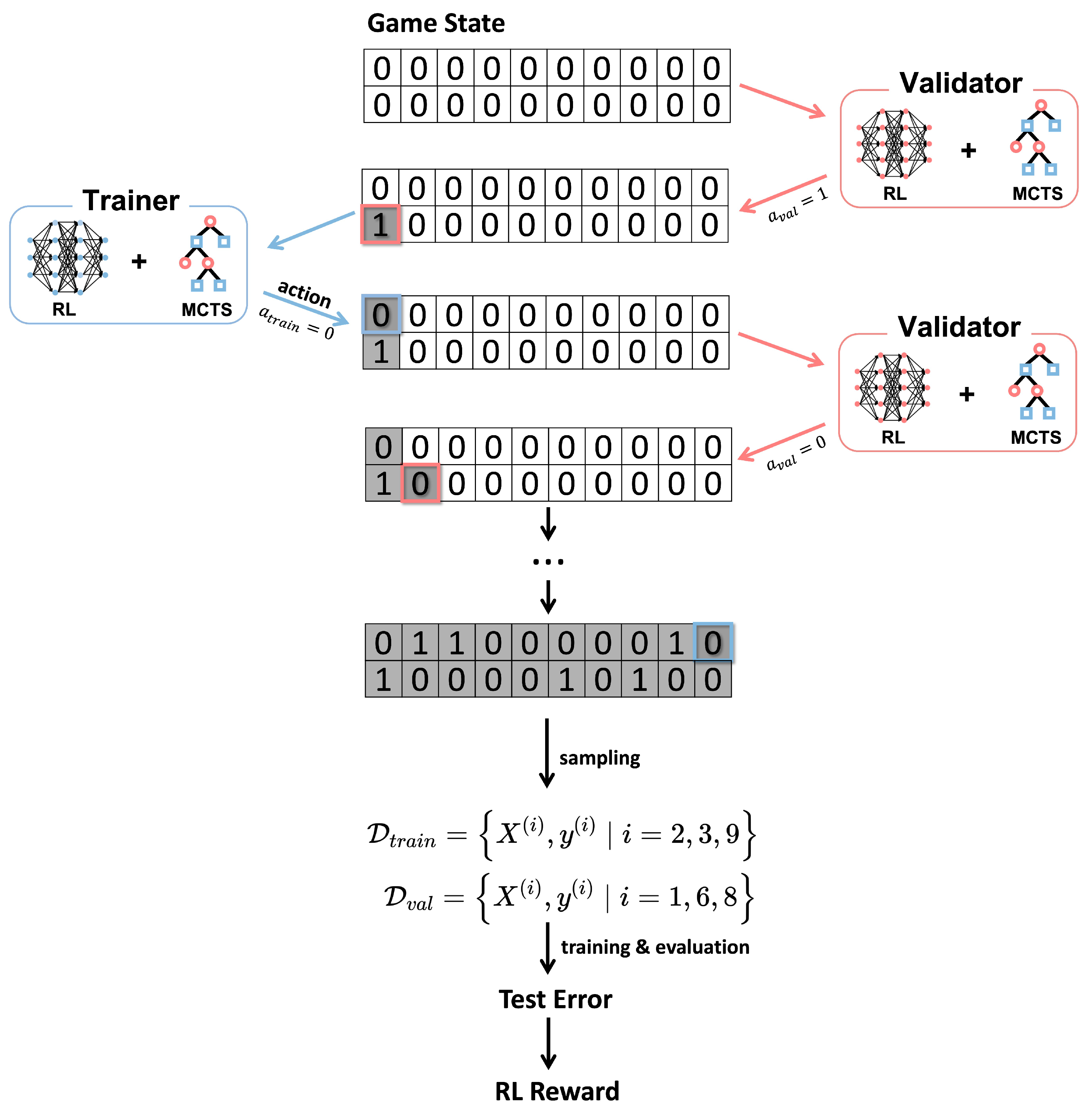
We formulate the sampling process as a two-player game, which is illustrated in Figure 1. A trainer aims to select the training data that minimizes the test error, while the validator selects the validation data to maximize the test error. The purpose of the validator is to provide adversarial examples during the training process so as to enhance the model generalizability. The game information, including each player’s move and the game result, is stored to update the strategy of each player. After several rounds of games and the convergence of the player’s strategy, the equilibrium is achieved so that the optimal data set components and sizes (i.e., N t r a i n and N v a l ) are determined.
The game starts with empty training and validation sets, and the trainer and validator take turns to select or skip the next data point (i.e., next feature-label pair) until all data points have been chosen. Below is an example game built on a small dataset with 10 data points in total. The validator moves first by selecting the first data points into the validation sets, and the trainer then decides to skip the first data. The validator moves on according to the historical moves of both the trainer and validator. After 10 turns, the validator selects the 1st, 6th, and 8th data points into the validation set D v a l , and the trainer selects the 2nd, 3rd, and 9th data points into the training set D t r a i n . The training and evaluation processes are followed to calculate the reward, which will be used to update the trainer and validator. In the remainder of this section, we will introduce the details of the two-player game, including its states, actions, rules and scores. The architecture of each game player, which contains reinforcement learning (RL) and Monte Carlo tree search (MCTS) components, will also be detailed.

3.2.1. Game State

The game is fully observed, i.e., both the training and validation player has access to the historical data selection. The current game state can be mathematically represented as a binary indicator vector s = [ t 1 , , t N , v 1 , , v N ] to indicate whether the corresponding training and validation data points are selected, where N is the size of the dataset, i = 1 N t i = N t r a i n and i = 1 N v i = N v a l . For example, t 1 = 1 means the 1st data point is selected into the training set, i.e., D ( 1 ) D t r a i n . In the initial state, all elements of the game state are 0.

3.2.2. Game Action

In the example game, the actions of both players are the same: given the current state, each player chooses whether to select the next data point or not. We denote the action set as A = { 0 , 1 } , where 0/1 indicates selecting/skipping the next data. Each player starts with the first data, which corresponds to the leftmost side of the dataset, and determines the choice of the next data by outputting the action a A . The player policy, i.e., the probability of each action set element to be selected, will be discussed later as shown in Equation (4).
The player will not have legal moves when all data has been traversed, and the game stops when both players don’t have any legal moves. The final state records our data selection.

3.2.3. Game Rule

The game is initialized with an empty game state. The game starts with the validator making the first move. Each player determines the action to select/skip the next data, starting from the leftmost data point (i.e., D ( 1 ) ). After making the selection, the current player is switched. The game terminates when both players have considered all the data, and the selected data is applied to train the model f, which will then be evaluated using the holdout test set.

3.2.4. Game Score

In the example game, the mean squared error (MSE) is used to evaluate the performance of the model, and thus can be considered as a score to evaluate the data selection. If the score is high, the validator wins the game, and vice versa. Then, a non-trivial question is how to determine the MSE threshold for claiming a winner. In contrast with traditional two-player games, like chess and go games, the trainer and validator play asymmetric roles in the game of sampling data. To address the matter, we first measure the average test MSE of a random sampler, which we call the base MSE. We claim the trainer (validator) as the winner if the test MSE is significantly lower (higher) than the base MSE. Suppose our two players play randomly for sufficient games; the test MSE of the trained model is then a random variable, denoted as M = i N t e s t | y t e s t ( i ) f ( X t e s t ( i ) | θ * ) | 2 / N t e s t , where θ * is the optimal parameter. The test MSEs of different games are independently and identically distributed. The expectation of M, which is in fact the base MSE, should be a moderate value because both players lack intelligence, and thus there is no guarantee one could always outperform the other. To win the game, the test MSE should be significantly higher (for validator) or lower (for trainer) than the base MSE E ( M ) . In practice, we use the mean of M to approximate E ( M ) : M i / n E ( M ) , where n is the number of games played.
Another non-trivial question is that, in implementation the player may use as much data as possible, which is a conservative policy. However, the redundant data will incur computation costs and also may hide the essential one. To solve that, we penalize the amount of data each player chooses. We encourage both players to choose as little data as possible while trying to win the game. The benefit of this trick is to unveil the most optimal and efficient data points. Our score definitions are as follows:
S t r a i n = M S E + α | | s | | 0 S v a l i d = M S E α | | s | | 0
where s is the final game state, α controls the penalty for the selected data size, and | | · | | 0 is the L 0 norm that computes the number of non-zero elements. It is hard to find a unified form of the score for both the trainer and validator because they have opposite targets. Therefore, scores are calculated for both the trainer and validator separately, and the means of scores after sufficient games are S ¯ t r a i n = i = 1 n S t r a i n ( i ) / n and S ¯ v a l i d = i = 1 n S v a l i d ( i ) / n for the trainer and validator, respectively.

3.2.5. Game Reward

The game reward, usually ranging from −1 to 1, describes how favorable the game outcome is towards each player. As two players in our game play competitively, the rewards for the trainer and validator are opposite. We adopt a mapping function to convert the scores to rewards. Let S t r a i n n e w and S v a l i d n e w denote the score of a new game. If both the scores are bigger or lower than the average scores S ¯ t r a i n and S ¯ v a l i d by a tolerance, we may announce a winner, and reward for the winner is +1 and for the loser is −1. Otherwise, the game result is a tie. The reward is defined as follows:
  • If S t r a i n n e w < S ¯ t r a i n t o l and S v a l i d n e w < S ¯ v a l i d t o l , then r e w a r d t r a i n = 1 and r e w a r d v a l i d = 1
  • If S t r a i n n e w > S ¯ t r a i n + t o l and S v a l i d n e w > S ¯ v a l i d + t o l , then r e w a r d t r a i n = 1 and r e w a r d v a l i d = 1
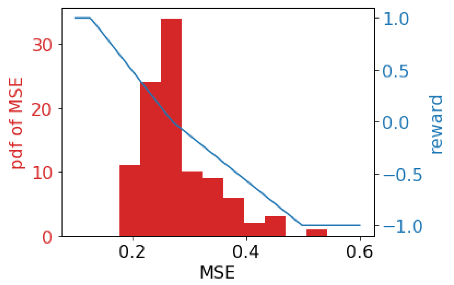
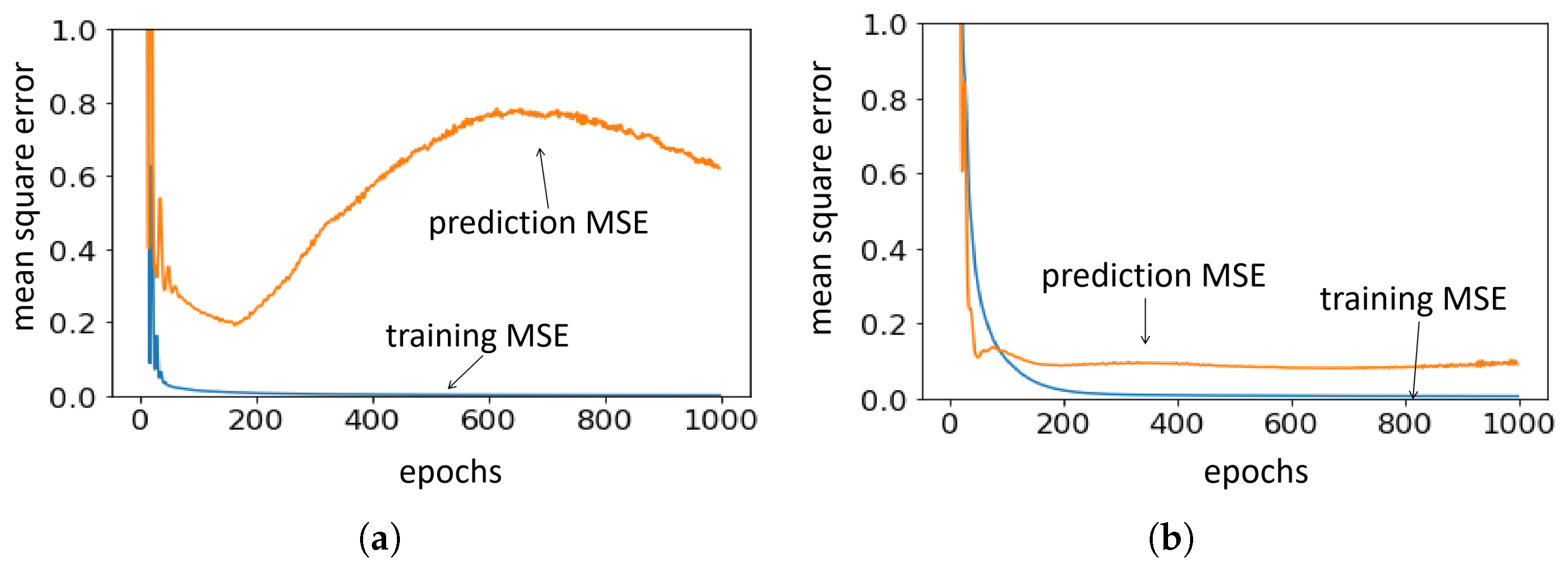
  • Otherwise, a piece-wise linear function is adopted to map the score to the reward, which is shown in Figure 2. We randomly sample the training and validation data, then train and evaluate a CF model (the CF model will be introduced in Section 4), and Figure 2 shows the distribution of the test MSE (left y-axis). The blue line shows the piece-wise mapping function of the reward (right axis), and the validator’s score-to-reward mapping is the opposite of the trainer.
The range of t o l is the same as the average scores S ¯ t r a i n and S ¯ v a l i d . Otherwise, if t o l is too large, most games will end up with draws and return zero rewards; if t o l is too small, a win with a narrow margin will receive a high reward value, imposing fluctuation on the game results. In experiments, t o l is a hyperparameter to tune.

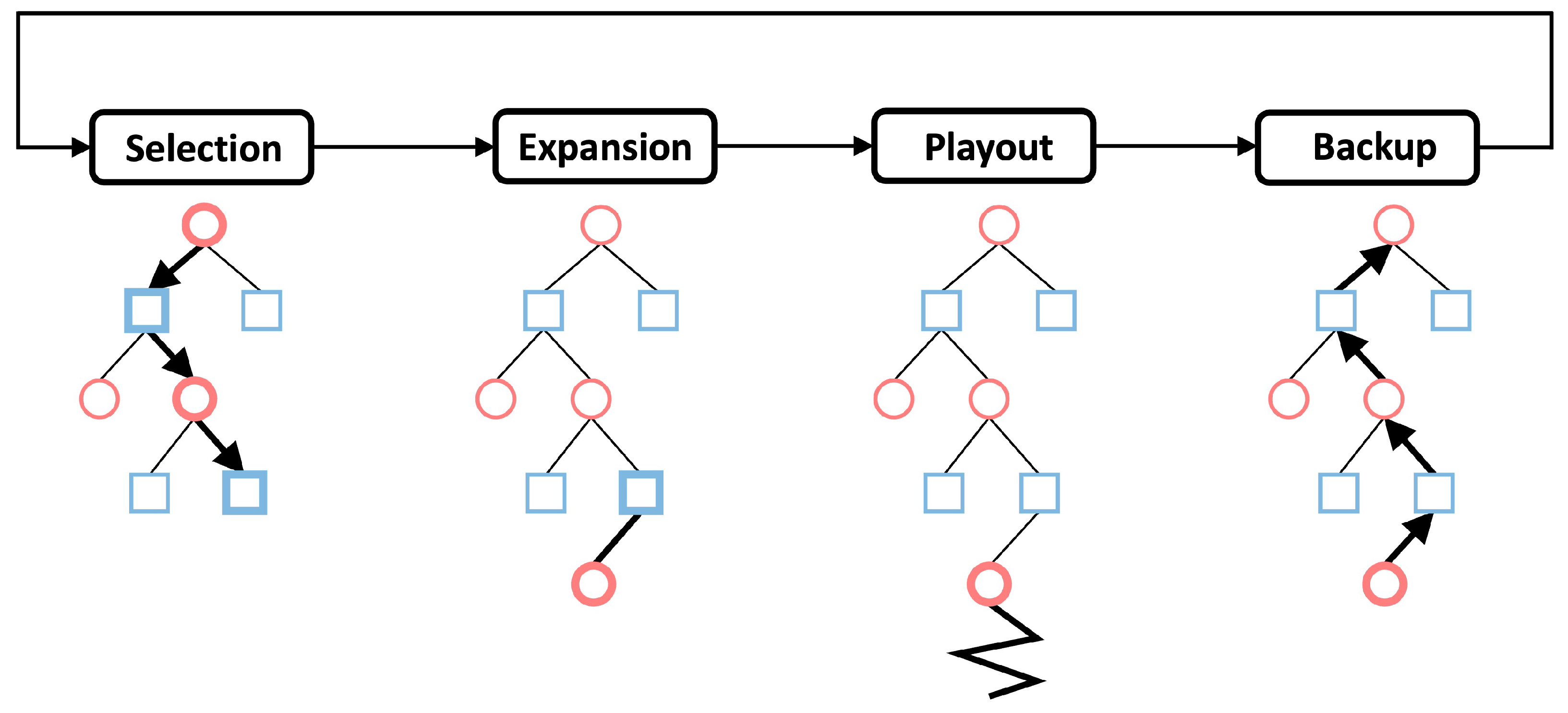
3.3. Monte Carlo Tree Search (MCTS)

In avoidance of myopic and greedy moves, a player always chooses its next action considering its opponent’s future moves. In other words, each player solves a search problem, where the size of the search tree grows exponentially if multiple moves ahead are taken into consideration. To tackle this issue, MCTS iteratively explores the searching space, and gradually adjusts its exploration towards the most promising region. Below, we briefly introduce the tree components before moving on to the tree search strategy.
A node s represents the state of the game at a certain stage. For example, a root node represents the initial game state with empty training and validation sets, and a termination node represents the final game state where the training and validation sets are sampled. All nodes, except for the termination node, connect to their children nodes through edges, which represent actions of the current player. A tree starts with the root node as its only component and grows by appending one child node. The newly added child node is called a leaf node, and it turns into a non-leaf node if one of its children nodes is also appended to the tree. Note that either the leaf or non-leaf attribute is specifically for the existing nodes of the tree. The termination node is not a leaf node until it is visited and appended to the tree.
The search iteration (Figure 3) involves traversing the existing tree from the root node to one leaf node, together with extending the tree by appending a new leaf node. In Figure 4, the red circle means the current player is the validator, and the blue square means the current player is the trainer. Specifically, each iteration includes four phases:
  • Selection. The first phase starts with the root node and sequentially selects the next node to visit until a leaf node is encountered. Each selection is based on:
    SELECT argmax a { r ¯ ( s , a ) + c puct b n ( s , b ) 1 + n ( s , a ) } ,
    where r ¯ ( s , a ) is the average reward gathered over all tree-walks, n ( s , a ) is the number of visit of edge a, and b n ( s , b ) is the number of visit of node s. c p u c t is a constant determining the level of exploration.
  • Expansion. When a leaf node is encountered, one of its children nodes is appended and the tree thus grows.
  • Playout. After the expansion phase, a random playout is used to finish the remaining search. That is, each player will randomly move in the rest of the game the termination node is reached and computing the associated reward.
  • Backup. The node and edge statistics are updated in the last phase of a searching iteration. First, the number of the visit of all traversed nodes and edges are incremented by one. Second, the current reward computed in the playout phase is back-propagated along the traversed path, and is used to update the average reward r ¯ ( s , a ) .
After the statistics of the nodes and edges are finished being backed up, MCTS starts the next iteration from the root node. The searching process terminated when the number of iterations reaches a preset value n u m I t e r s , which is tuned to allow the game to reach equilibrium while avoiding excessive iterations. Then, the current player makes its next move based on the following policy
π ( a | s ) = n ( s , a ) 1 / τ b n ( s , b ) 1 / τ ,
where τ is a constant tunable hyperparameter that controls the level of exploration. A large τ encourages random move selection, and a small τ prefers the move with the highest number of visits. After that, the other player takes turns to continue the game.

3.4. Reinforcement-Learning-Aided MCTS (RL-MCTS)

Taking inspiration from AlphaGo Zero [19], we adopt reinforcement learning (RL) to further narrow down the searching space by gradually biasing the search to a more promising region.

3.4.1. Value Network

The key idea of applying RL to MCST is to replace the random and time-consuming playout with a function evaluation. When a leaf node is encountered, the current player approximates the average reward by a surrogate model instead of using the random playout. We employ two value network q θ T ( s , a ) and q θ V ( s , a ) for the trainer and validator, respectively. The networks take in the game state and action, and return the position value for the current player. We use the replay buffer to train the value network, where the states traversed together with the game results are fed into the value network as the training examples. As introduced in Section 2, the difference between two networks is that they are fed with different rewards after the game is completed.

3.4.2. MCTS with Value Networks

Aided with RL, the RL-MCTS processes are updated as follows
  • Selection. Each selection is based on:
    SELECT argmax a { q θ ( s , a ) + c puct b n ( s , b ) 1 + n ( s , a ) } .
    Compared with Equation (3), the difference of RL-MCTS’s selection phase is that the average reward is replaced with the evaluation of the value function.
  • Expansion. This phase is the same as the MCST.
  • Playout. The reward attained from a random playout is replaced with the evaluation of the q value function.
  • Backup. The backup is the same as the MCTS, except for that the q value rather than the average reward is the statistic to be updated.

3.5. Summary

The architecture consisting of a simulation platform and the two player game is bi-level. The trainer and validator play the sequential competitive game. After the game is finished and the data is generated, the test MSE is calculated at the simulation level, in which a neural network CF model is trained with the trainer’s data and validated by the validator’s data. The reward is then computed by the pre-defined rules and returned to the game level as the target for training the value network. The whole process is shown in Algorithm 1.
Algorithm 1: Two-player game
Input: The components of the two-player game defined in Section 3.
Output: Two trained value networks for both players, which will manage to evaluate the current position according to the current player.
     Initialization:
1:
Initialize empty sets of the training examples for the value network of trainer and tester: t r a i n E x a m p l e s [ ] , v a l i d E x a m p l e s [ ] .
2:
Set the board limit for both players: p o s L i m i t s = [ n , n ]
3:
fori in [0, ..., n u m I t e r s − 1] do
4:
    Empty the game state: s = [ 0 , , 0 n , 0 , , 0 n ]
5:
    Initialize the current player: c u r r e n t P l a y e r = 1 (1 for tester, 0 for trainer).
6:
    Initialize the current position for the trainer and tester to be the leftmost position: p o s T r a i n V a l i d = [ 0 , 0 ] .
7:
    Initialize empty tree of the Monte Carlo Tree Search, set the hyperparameter τ = 1 for “exploration and exploitation”
8:
    while True do
9:
        
10:
        if  p o s T r a i n V a l i d [ c u r r e n t P l a y e r ] > = p o s L i m i t s [ c u r r e n t P l a y e r ]  then
11:
            c u r r e n t P l a y e r = 1 c u r r e n t P l a y e r + 1 . Continue to the next loop
12:
        end if
13:
        Check for all legal actions at current state s according to the game rules.
14:
        Given current state s, get the action probabilities π ( s , · ) for all legal actions by performing n u m M C T S S i m s times of MCTS simulations.
15:
        Sample action a { 0 , 1 } from probabilities π ( s , · ) .
16:
        
17:
        if  c u r r e n t P l a y e r = = 0  then
18:
             s [ p o s T r a i n V a l i d [ c u r r e n t P l a y e r ] ] = a
19:
        else
20:
             s [ p o s T r a i n V a l i d [ c u r r e n t P l a y e r ] + m ] = a
21:
        end if
22:
        if  p o s T r a i n V a l i d = = p o s L i m i t s  then
23:
            break
24:
        end if
25:
    end while
26:
    Evaluate the score for the trainer and tester.
27:
    Evaluate the reward r for trainer and tester.
28:
    Append the history in this game episode [ s , a , r ] to t r a i n E x a m p l e s and v a l i d E x a m p l e s
29:
    Train the value networks q θ T and q θ V with t r a i n E x a m p l e s and v a l i d E x a m p l e s . The trained networks are used in the next game.
30:
end for

4. Case Study: Car-Following Modeling

To evaluate the performance of our proposed sampling method in training ML models, we train a neural network CF model, denoted as f θ , as a demonstration. The structure of the CF model is shown in Figure 4.
The neural network takes the velocity, velocity difference, and the headway of current time as the input, and returns the target acceleration for the next time step. According to the general neural network model that is mentioned in the literature review, we use neural network architecture shown in Figure 4. The v f t , Δ v t , and Δ x t are the follower’s velocity, velocity difference between follower and leader, and space headway at time t. Those values are called the s t a t e of the follower.
As for modeling the nonlinearity of car-following behaviours, we chose the Rectified Linear Unit (ReLU) as the activation function in this neural network model. The equation is as follows:
h m , n = Re LU W m , n x + b m , n = W m , n x + b m , n ; x > 0 0 ; x 0 ,
where h m , n denotes the nth hidden unit in the mth hidden layer, W m , n and b m , n are the weight matrix and bias for h m , n , and x is a vector of all inputs from the last layer.
As the acceleration is normally between −3 m/s2 and 3 m/s2, we add a Hyperbolic Tangent Layer to constrain the scale of output acceleration. The Hyperbolic Tangent activation function is defined as:
a ^ t = t a h n ( W m , n x + b m , n ) = 3 ( 2 1 + e 2 ( W m , n x + b m , n ) 1 )
where a ^ t is the output acceleration at time t, x is a vector of all input from the last hidden layer in this architecture.

4.1. Data Description

The data is from the Next Generation Simulation (NGSIM) project, a national project aiming at helping develop algorithms and datasets for the calibration and validation of traffic models.
The NGSIM freeway database consists of vehicle trajectories on two test sites. The I-80 test section is a 0.4-mile six-lane freeway. The processed data include 45 min of vehicle trajectories in transition (4:00–4:15 p.m.) and congestion (5:00–5:30 p.m.). The US101 site is a 0.3 mile weaving section with five lanes. The processed data include 45 min of vehicle trajectories in transition (7:50–8:05 a.m.) and congestion (8:05–8:35 a.m.). The data have been extracted from video recordings using machine vision algorithms.
The oscillation area only counts a few parts for the whole dataset, but is hard to predict very well. Here we take a closer look at this problem, with the aim of intelligently choosing data for a stable, robust model.
The whole dataset we select consists of nine trajectory segments from free flow and one trajectory segment from the oscillation area, which is consistent with the fact that the oscillation data count only for a limited part of data in the NGSIM dataset and other naturalistic datasets. The duration of these data is from 10 s to 15 s. To validate the performance of the model, we choose a relatively complete trajectory, where the free flow, acceleration, and deceleration share the almost same ratio.
The goal of this experiment is twofold: (1) to verify the ability to select data for both players. This ability is verified by alternative activating one player and deactivating another, and the active player will outplay (increasing prediction MSE for trainer and decreasing MSE for validator) the other. (2) to verify the data generated from the alternative play mentioned above is help to train a more stable model. The essence is that the role of the validator is to explore the data which the trainer may ignore, and the trainer would find more data to make up for it in the next turn. In this way, the model will less likely to overfit on the majority genre of data, which in our case is the free-flow scenario.

4.2. Experiment Setting

We train two network car-following models with identical configurations, one denoted as f θ B that is trained with randomly sampled data, the other denoted as f θ G that is trained with RL-MCTS-sampled data. Both networks have three hidden layers, the size of which is 64, 64, and 32. The only difference is the data we feed into them. To expedite the self-play process, we set the n u m M C T S S i m to only two. The Adam optimizer is used to train the neural networks.

4.3. Results

Figure 5 presents the model stability comparison. The left and right figures are the error curves of the random and RL-MCTS sampling methods, respectively. The x-axis is the training epoch and the y-axis is the test MSE. We can see that when training the model with the randomly sampled data, the model overfits and the prediction MSE spikes during the training. When training the model with the RL-MCTS sampled data, the overfitting is mitigated, and both the training and test errors converge. This can be explained because the RL-MCTS sampled training data already considers the data heterogeneity and thus is less vulnerable to overfitting. To demonstrate that, Figure 6 compares the velocity distributions of two sampling methods, the left and right for the random and RL-MCTS sampling, respectively. The x-axis is the vehicle velocity and the y-axis is the probabilistic density. We can see that the randomly sampled data clearly contains the major velocity and the minor velocity, which also reflect the naturalistic velocity distribution of the human driving data. The data sampled by RL-MCTS as a more balanced distribution, which can help mitigate the overfitting.
Apart from the result illustration of one sampling, we are more interested in the overall performance of several rounds of sampling. Thus, we repeat each experiment 100 times with both the random and RL-MCTS sampling. The distributions of the test MSE and reward are shown in Figure 7, where the blue and orange stand for the RL-MCTS and the random sampling, respectively. We can see that model trained using the RL-MCTS sampled data is more robust towards the data randomness.

5. Conclusions

The prediction performance of ML models depends on their training and validation datasets. Thus, the strategic selection of training and validation datasets is crucial for the robustness of the trained models. A case study of modeling human car-following driving behavior has been understudied. This paper aims to develop an AI-guided experiment design framework in which training and validation datasets are strategically selected so that the model prediction performance can be optimized. We consider a CF modeling problem comprised of three intelligent players, namely, the training data selector, and the validation data selector, each of whom has different objectives. The training data selector and the validation data selector play a non-cooperative game on the upper level as leaders. The trainer aims to minimize the MSE of the estimated model outputs, while the validator aims to maximize MSE to ensure the predictive power of the trained model. The action spaces of the training data selector and the validation data selector are 0,1, standing for whether to choose the next data or not. This is essentially a combinatorial problem. To reduce the action search space, RL-aided MTCS is applied. We test the developed algorithm using the neural network car-following model.
We select an optimal combination of training and validation datasets that achieves the highest robustness of the model. The result shows that if we resample the original dataset in the training step and add more weights to those data which will impair the model performance, the model will become more robust.
This work provides an approach to robustly and efficiently exploit real-world long-tail data. By training each player in a competitive game and penalizing the data size, the most critical data points are discovered. The result indicates a potential application in the real-world training and deployment of ML models, where the discovered critical data can help accelerate the training process and reduce computational time.
Albeit novel, this work can be extended in the following ways:
  • We have only verified the algorithm in a small dataset. We can apply this algorithm to a bigger dataset with diverse characteristics.
  • Transforming the original one-shot problem to a sequential one will lead to a sub-optimal solution. This problem can be addressed if we allow the player to retract a false move.

Author Contributions

Conceptualization, Z.M. and X.D.; methodology, Z.M. and R.S.; validation, Z.M.; formal analysis, Z.M.; writing—original draft preparation, Z.M.; writing—review and editing, X.D.; supervision, X.D. and R.S.; funding acquisition, X.D. All authors have read and agreed to the published version of the manuscript.

Funding

This research is partially sponsored by the National Science Foundation (NSF), United States under NSF CPS-2038984.

Data Availability Statement

Not applicable.

Conflicts of Interest

We confirm that neither the manuscript nor any parts of its content are currently under consideration or published in another journal. All authors have approved the manuscript and agree with its submission to the journal “Games.”

References

  1. Fu, Y.; Xiang, T.; Jiang, Y.G.; Xue, X.; Sigal, L.; Gong, S. Recent advances in zero-shot recognition: Toward data-efficient understanding of visual content. IEEE Signal Process. Mag. 2018, 35, 112–125. [Google Scholar] [CrossRef]
  2. Mo, Z.; Shi, R.; Di, X. A physics-informed deep learning paradigm for car-following models. Transp. Res. Part C Emerg. Technol. 2021, 130, 103240. [Google Scholar] [CrossRef]
  3. Mo, Z.; Fu, Y. TrafficFlowGAN: Physics-informed Flow based Generative Adversarial Network for Uncertainty Quantification. In Proceedings of the European Conference on Machine Learning and Data Mining (ECML PKDD), Bilbao, Spain, 13–17 September 2022. [Google Scholar]
  4. Shi, R.; Mo, Z.; Huang, K.; Di, X.; Du, Q. A physics-informed deep learning paradigm for traffic state and fundamental diagram estimation. IEEE Trans. Intell. Transp. Syst. 2021, 23, 11688–11698. [Google Scholar] [CrossRef]
  5. Shi, R.; Mo, Z.; Di, X. Physics-informed deep learning for traffic state estimation: A hybrid paradigm informed by second-order traffic models. In Proceedings of the AAAI Conference on Artificial Intelligence, Virtual, 2–9 February 2021; Volume 35, pp. 540–547. [Google Scholar]
  6. Ossen, S.; Hoogendoorn, S.P. Validity of trajectory-based calibration approach of car-following models in presence of measurement errors. Transp. Res. Rec. 2008, 2088, 117–125. [Google Scholar] [CrossRef]
  7. Hoogendoorn, S.; Hoogendoorn, R. Calibration of microscopic traffic-flow models using multiple data sources. Philos. Trans. R. Soc. A Math. Phys. Eng. Sci. 2010, 368, 4497–4517. [Google Scholar] [CrossRef] [PubMed]
  8. Fernández, A.; Garcia, S.; Herrera, F.; Chawla, N.V. SMOTE for learning from imbalanced data: Progress and challenges, marking the 15-year anniversary. J. Artif. Intell. Res. 2018, 61, 863–905. [Google Scholar] [CrossRef]
  9. Tokdar, S.T.; Kass, R.E. Importance sampling: A review. Wiley Interdiscip. Rev. Comput. Stat. 2010, 2, 54–60. [Google Scholar] [CrossRef]
  10. Kantarcıoğlu, M.; Xi, B.; Clifton, C. Classifier evaluation and attribute selection against active adversaries. Data Min. Knowl. Discov. 2011, 22, 291–335. [Google Scholar] [CrossRef] [Green Version]
  11. Liu, X.; Hsieh, C.J. From adversarial training to generative adversarial networks. arXiv 2018, arXiv:1807.10454. [Google Scholar]
  12. Liu, G.; Khalil, I.; Khreishah, A. GanDef: A GAN based Adversarial Training Defense for Neural Network Classifier. In Proceedings of the IFIP International Conference on ICT Systems Security and Privacy Protection, Lisbon, Portugal, 25–27 June 2019; Springer: Berlin/Heidelberg, Germany, 2019; pp. 19–32. [Google Scholar]
  13. Browne, C.B.; Powley, E.; Whitehouse, D.; Lucas, S.M.; Cowling, P.I.; Rohlfshagen, P.; Tavener, S.; Perez, D.; Samothrakis, S.; Colton, S. A survey of monte carlo tree search methods. IEEE Trans. Comput. Intell. AI Games 2012, 4, 1–43. [Google Scholar] [CrossRef] [Green Version]
  14. Zhou, M.; Qu, X.; Li, X. A recurrent neural network based microscopic car following model to predict traffic oscillation. Transp. Res. Part C Emerg. Technol. 2017, 84, 245–264. [Google Scholar] [CrossRef]
  15. Sharma, A.; Zheng, Z.; Bhaskar, A. Is more always better? The impact of vehicular trajectory completeness on car-following model calibration and validation. Transp. Res. Part B Methodol. 2019, 120, 49–75. [Google Scholar] [CrossRef]
  16. Wang, X.; Jiang, R.; Li, L.; Lin, Y.; Zheng, X.; Wang, F.Y. Capturing car-following behaviors by deep learning. IEEE Trans. Intell. Transp. Syst. 2017, 19, 910–920. [Google Scholar] [CrossRef]
  17. Zhu, M.; Wang, X.; Wang, Y. Human-like autonomous car-following model with deep reinforcement learning. Transp. Res. Part C Emerg. Technol. 2018, 97, 348–368. [Google Scholar] [CrossRef] [Green Version]
  18. Nageshrao, S.; Tseng, E.; Filev, D. Autonomous Highway Driving using Deep Reinforcement Learning. arXiv 2019, arXiv:1904.00035. [Google Scholar]
  19. Silver, D.; Schrittwieser, J.; Simonyan, K.; Antonoglou, I.; Huang, A.; Guez, A.; Hubert, T.; Baker, L.; Lai, M.; Bolton, A.; et al. Mastering the game of go without human knowledge. Nature 2017, 550, 354. [Google Scholar] [CrossRef] [PubMed] [Green Version]
  20. Wang, K.; Sun, W.; Du, Q. A cooperative game for automated learning of elasto-plasticity knowledge graphs and models with AI-guided experimentation. Comput. Mech. 2019, 64, 467–499. [Google Scholar] [CrossRef]
Figure 1. Illustration of sampling training and validation sets as a two-player game.
Games 14 00013 g001
Figure 2. Score-reward mapping function of the trainer.
Games 14 00013 g002
Figure 3. Illustration of MCTS.
Games 14 00013 g003
Figure 4. Neural network CF model.
Games 14 00013 g004
Figure 5. Error curves of the random (a) and the proposed sampling method (b).
Games 14 00013 g005
Figure 6. Velocity distributions of the random (a) and the proposed (b) sampling.
Games 14 00013 g006
Figure 7. Comparison of the scores (a) and reward (b) between random and the proposed sampling methods.
Games 14 00013 g007
Disclaimer/Publisher’s Note: The statements, opinions and data contained in all publications are solely those of the individual author(s) and contributor(s) and not of MDPI and/or the editor(s). MDPI and/or the editor(s) disclaim responsibility for any injury to people or property resulting from any ideas, methods, instructions or products referred to in the content.

