1. Introduction
TinyML/Embedded Intelligence is a research field dedicated to implementing Machine Learning (ML) techniques in Embedded Systems, the core of all devices at the end of the network. Embedded systems have more limitations than Cloud computers [
1,
2]. The main focus is to empower such devices to perform intelligent tasks that were once developed for computers. This implementation reduces the need for a Cloud computer to perform all the intelligent layer tasks and creates more autonomous systems [
3,
4]. However, there are Embedded Systems that are more limited in terms of memory and processing than others, which are called Resource-Scarce Embedded Systems (RSESs). The memory and clock speed of an RSES are under 1 GB and 1 GHz, respectively. To implement an intelligent system, one has to optimize such ML models and techniques to fit the constraints of an RSES [
5].
Because more IoT devices are being broadly deployed with intelligent applications on them, obtaining solutions to understand whether the data being gathered by the device are similar to those used during the training phase is of great importance for post-deployment ML verification, sometimes known as outlier detection [
6]. Outlier detection is vital to determine whether a model running on specific hardware or in a certain environment will perform accordingly to expectations. Fields of study such as healthcare commonly use such techniques to verify if previous models can be transposed for new studies [
7]. As discussed in
Section 2.4, common techniques for verification are Data Distribution drift verification and outlier detection. However, in the last few years, with the advent of big data, Topological Data Analysis (TDA) has gained the attention of multiple users, and this novel approach is intended for use in RSES ML post-deployment verification systems.
TDA reduces a dataset to its topological features, allowing it to compare multiple datasets, understand its shape, and even find abnormalities. It reduces a dataset to its simplicial space, where connecting samples creates shapes, such as points, holes, tetrahedrons, and other geometrical shapes. It builds such shapes by grouping samples using a distance metric, where points with a distance of less than
r from each other are considered connected [
8,
9]. However, the problem with TDA resides in the decision of the best
r to use. Persistent Homology (PH) mitigates part of this problem. PH builds diagrams through iterative increases of
r, starting at 0. Then, it counts the number of
D-dimensional holes in each
r, storing the information regarding the birth of a new
D-dimensional hole or its death (when it fills itself). These PH Diagrams, known as birth–death diagrams, or barcodes, are snapshots that tell us about the lifespan of every topological feature [
10,
11,
12,
13].
Our previous work [
14] shows how to implement 0-Dimensional PH analysis in an RSES, considering a small number of samples. 0-Dimensional PH is the simplest method, because a simplicial complex is a point or a group of connected points, and a 0-dimensional hole is simply a line. Therefore, every simplicial complex is born at 0 and dies at
. The method is even able to fit RSESs such as the ARM Cortex-M0+, and since the PL method deployed in this work is very simple, one can perform this type of analysis in this constrained device as well.
This work is built upon our previous work and intends to include the capability of calculating on-the-fly Persistence Landscapes, which allows us to compare Persistent Diagrams [
15,
16]. After that, we show that if one looks at the landscapes obtained from multiple devices spread across a network, all landscapes converge to the same values. Therefore, by calculating the distance between the landscapes and setting a threshold, one can verify if a device is gathering samples from a distinct dataset shape.
1.1. Contributions
This works aims to show that the implementation of PL in an RSES is possible and that it is a helpful tool to verify, in real-time, the similarities between two or more datasets by developing an iterative method for the mean calculation of PL using cached samples. Therefore, this work contributions are the following:
The first implementation of 0-dimensional PL analysis in an RSES.
A post-deployment ML model data verification system using PL, which is helpful for TinyML/ Embedded Intelligence.
A mechanism to verify whether devices are collecting the same dataset, through dataset convergence verification, which is helpful in applications such as the Internet of Things (IoT); Wireless Sensor Networks (WSN); and Cyber-Physical Systems (CPS).
A reduction of the need for a central system (i.e., Cloud Computer) to analyze the entire dataset.
1.2. Organization of the Work
This work is organized as follows: In the introduction, the current section, we summarize the works related to the motivation of this paper regarding IoT healthcare services and present the motivations and objectives. In
Section 2, we present the data analysis. In
Section 3, we introduce the methodology of the work. In
Section 4, we present the experimental design with the setup metrics. In
Section 5, we present the results of this work and
Section 6 draw the conclusions of this work.
2. Topological Data Analysis (TDA)
Many fields of study use the TDA as an analysis tool to find solutions to their questions. These fields of study range from medical sciences to sensor networks. The interest in such analysis resides in the increasing amount of data and the necessity of finding meaningful insights about them. To do so, TDA uses methods from algebraic topology.
One of the TDA’s primary tools is Persistence Homology (PH), an algebraic method that recognizes topological features. PH achieves this goal by verifying how points in the dataset connect to build simplicial complexes. A point is said to be connected with another if two points have a distance of equal to or higher than r. For each r, a different number of shapes is formed. The question resides in knowing which r to choose.
To avoid choosing a random r, PH starts with and increases it, storing information about the birth and death of each simplicial complex for each r. Then, it counts the number of h-dimensional holes at each r, sometimes denominated as the Betti numbers (), to produce a persistent module.
2.1. Persistence Modules
Persistent Modules (PM) are the main focus of study in TDA. One can perceive a PM as a finite sequence of birth–death pairs:
, where
. This finite set of points is obtained from a point cloud,
, that exists in a plane
. If each point in
is replaced by a
-dimensional ball,
, of radius
r and centered in
(Equation (
1)), one obtains a set of unions,
, from where to withdraw our homology.
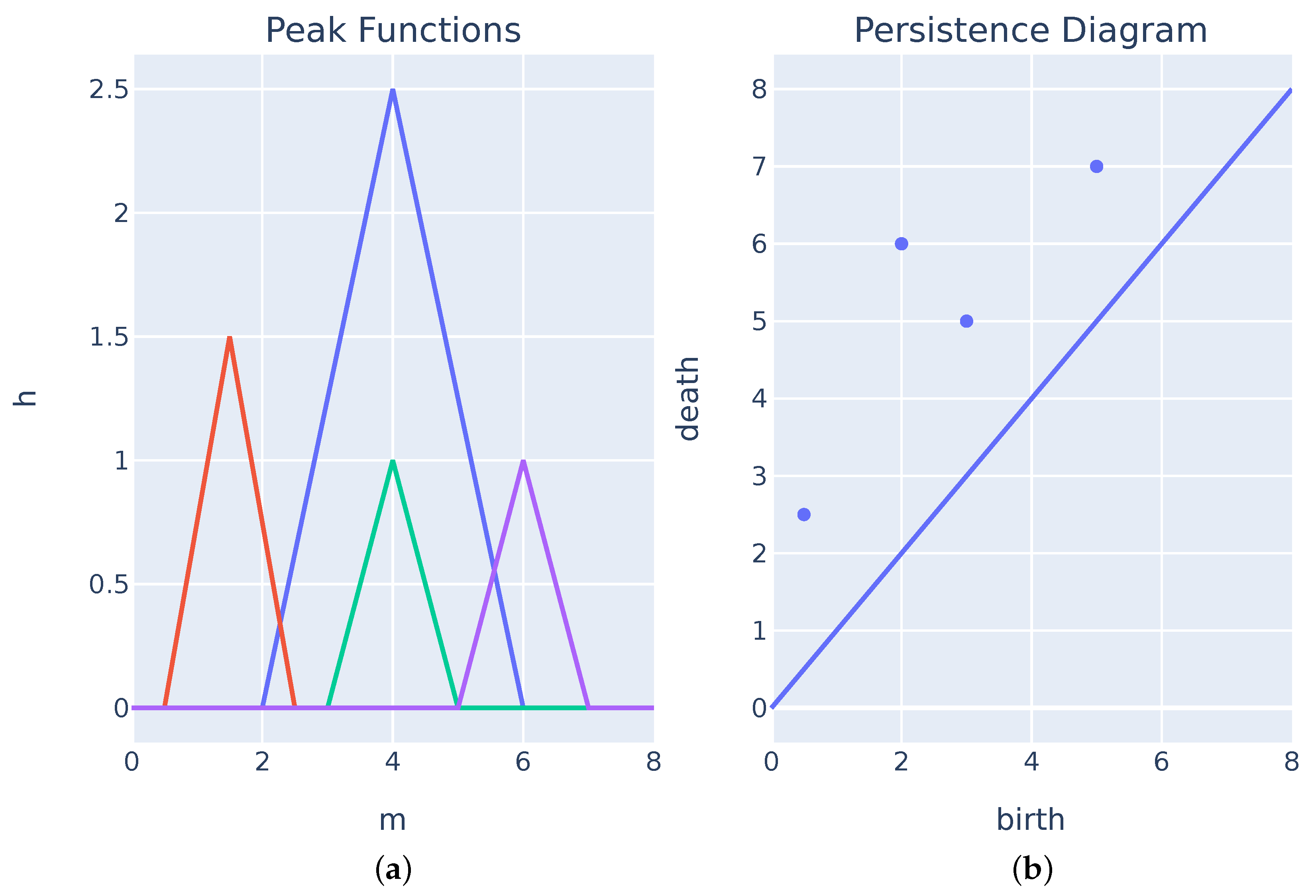
The finite set of birth–death pairs can be plotted into Persistence Diagrams, , or barcodes, that condense the entire PM study and provide us with information about the lifespan of each topological feature. The PD varies according to the homology dimension () one uses. The value provides information about the dimensions of the voids found, where means that a component dies whenever it connects to another. In contrast, means that the component dies when a 2-dimensional space (a circle) between a set of points is filled.
The main focus of this study is , because, as demonstrated before, it its simplicity allowed to make optimization to fit the RSES constraints. For , every component has its birth at 0 and dies when a connection is made with another component. This is essential information to have in mind because it will be the building stone of our solution.
Each point cloud will have a distinct
. One can use the bottleneck distance to verify the similarity between two PDs. The bottleneck distance between two PDs,
A and
B, is the maximum cost function’s value from all possible partial matches between the collection of pairs,
. Therefore, for each match, one considers a cost function
, Equation (
2), which is the
norm between the two points. For any unmatched pair,
is equal to
, where
b and
d are the birth and death coordinates for the unmatched point. The bottleneck is defined as the cost of the most efficient partial match (see Equation (
3)).
Because the bottleneck distance is the maximum of all possible sets and unmatched points, one can perceive it as being computationally expensive and messy to compute due to all the possible partial matches to compute.
However, one can perform another PD comparison using the Wasserstein Distance (WD), also known as the Earth’s mover distance. The WD gives us the work needed to transform one diagram into another. The WD equals the maximum
norm of all bijections between diagrams A and B, as shown in Equation (
4). For
, one obtains the Bottleneck Distance.
2.2. Persistence Landscapes
The main idea behind mapping a
to a set of persistence landscape functions (
) is to use a space in which the concept of the mean is well-defined, therefore allowing us to perform a pointwise comparison between datasets. To make such a mapping, one creates a set of peak functions
, where we let
One can use the piecewise function from Equation (
6) to create the peak functions from
.
Figure 1 shows the PD and its respective peak function. These peak functions have a value of zero everywhere except during the component’s lifespan and can be perceived as a 45 degree rotation of the Persistent Diagram.
From the peak function set
, one can now obtain the respective set of landscape functions,
, which are equal to
where, for each
, one can use the maximum values that are unused in
and so forth until
.
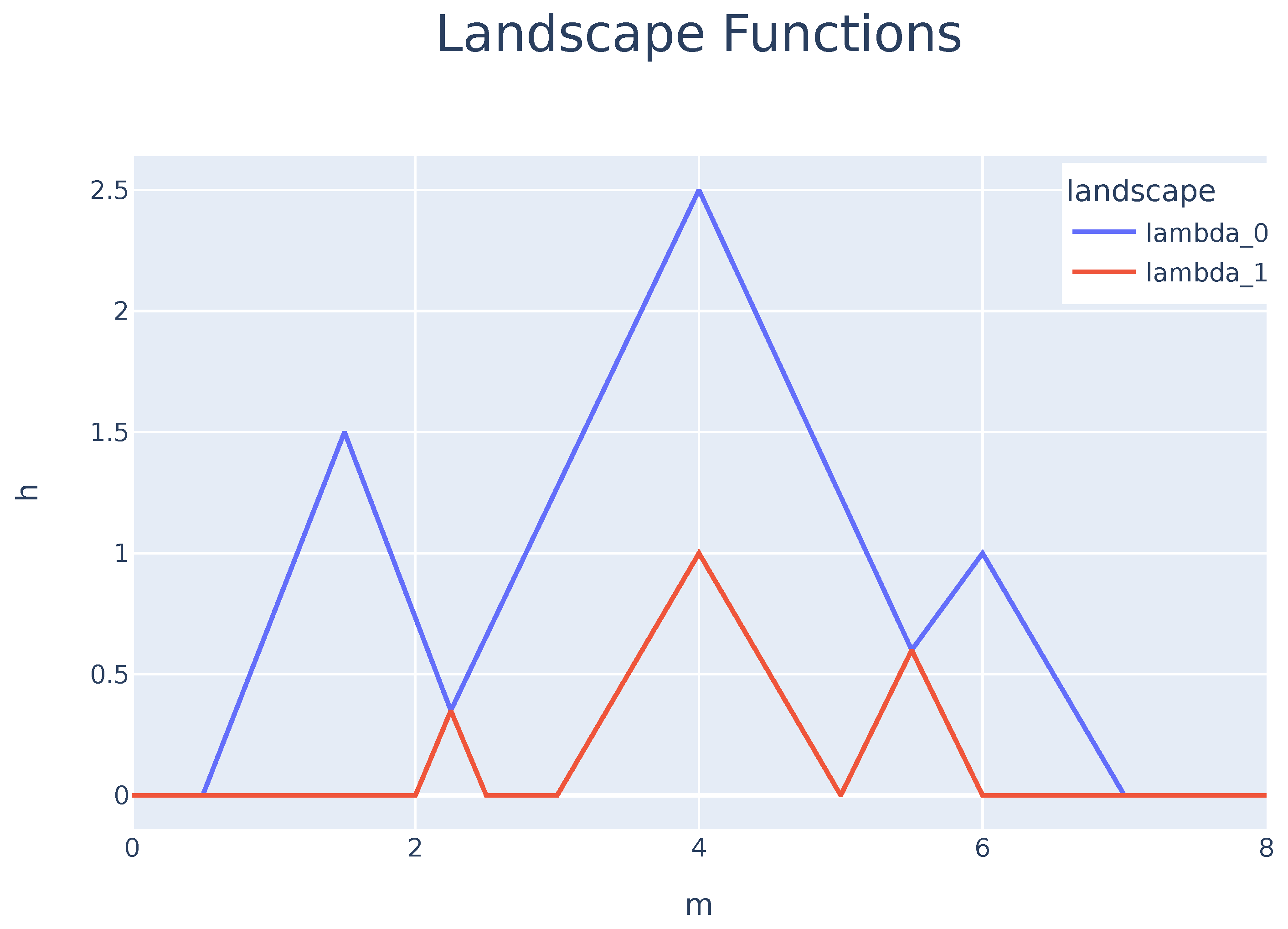
Figure 2 shows the set
obtained from the peak functions presented in
Figure 1. Using
, one can now determine the mean for every
function through
Persistence Landscapes have been used to solve problems or improve known analytical methods. The fields in which such tools are applied range from deep learning [
17] to microstructures [
18] and medical science [
19].
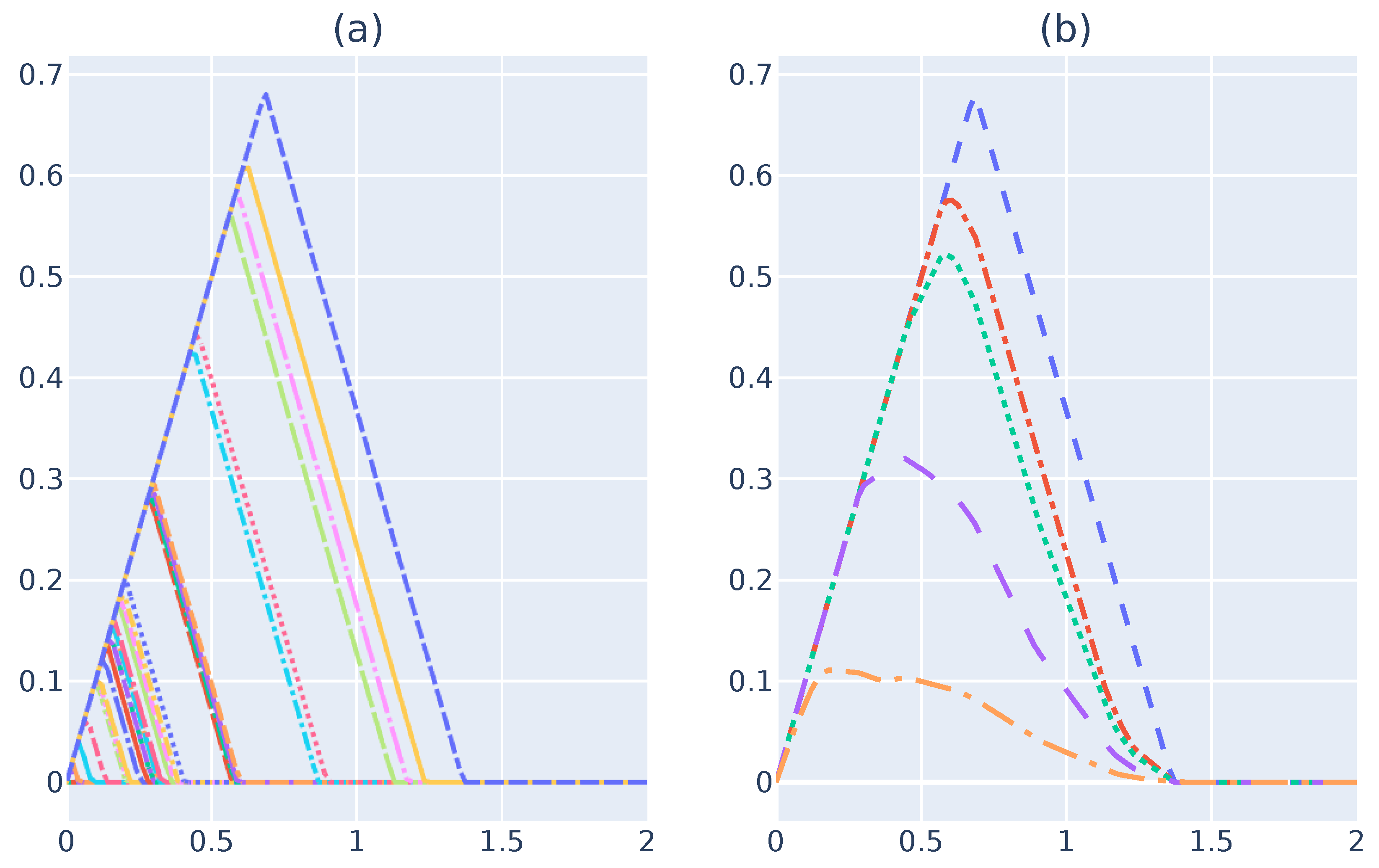
2.3. 0-Dimensional Persistence Landscapes
This entire work focus on building Persistent Landscapes for barcodes obtained by performing a 0-dimensional persistent homology analysis. There a few aspects in this dimension that are useful to pay attention to. Such aspects that facilitate Persistent Landscape building in an RSES,
Figure 3a illustrates the peak function drawn from a 0-dimensional barcode. As one can see, the peak functions share the left side of the triangle. The reason for such behavior is because, in
, every single point is a connected component, which means that every simplicial component is born at 0.
Because the peak functions for
are triangles inside one another and, as explained previously,
is a set composed of each triangle, since the maximum value at step
i will be the outside triangle, which is removed at step
. This property makes the Persistence Landscape set
equal to the peak function set
F and makes persistence landscapes at
simple to compute. Now, one can obtain
using Equation (
8). One can compute the entire set of
to determine the overall mean. However, in terms of the memory efficiency, one can identify the mean at each step
i to obtain a temporary value,
.
Figure 3b illustrates the result of
. At the end, one will obtain the same value as the value expected from computing all
values first. However, to do so, one must keep track of
i and multiply the previous
by
i before performing
.
Figure 3b illustrates
for each step.
This particular property for is essential to perform the calculations in an RSES due to their limited amount of memory, because it allows the landscape function and the mean calculation to be performed on-the-fly without having to keep too much data in the memory.
2.4. Related Work
The implementation of Persistence Landscapes is of great interest, and one can see this importance by the number of toolboxes and libraries that implement methods for PL analysis and calculation [
20,
21,
22,
23,
24]. The set of tools that exist is generic and developed for high-end computers and high-level programming languages, such as Python [
25] or Java [
26], whose memory and processing capabilities are many magnitudes greater than the smallest RSES tested, the Arduino M0 Pro, which has only 256 Kb of Flash, 32 Kb of SRAM, and a processor that runs at 48 MHz. Our method intends to fill this gap and optimize the existing methods to fit the memory and processing constraints of an RSES. However, they help to perform a higher dimensional homology analysis or verify the results obtained from the device. Multiple works have shown some Persistence Landscape properties maintain their stability, even in subsets of more extensive datasets and when their means converge [
16,
27]. However, in many of these tests, subsets of samples with lengths that are not suitable for comfortable processing in an RSES were used. This was shown to be 32 samples in our previous work, which means that a significant number of samples that hold enough information is needed for our method to provide any result that shows convergence.
In the literature, it one can find multiple works that intend to make post-deployment validations on a dataset to ensure that the ML model behaves correctly. Commonly used methods are created to detect outliers or drifts in the distribution. Sá et al. showed [
28] the importance of post-deployment validation of the dataset and sensor calibration for networks of devices gathering environmental data. In their extensive survey [
29], Ayadi et al. enumerated the challenges of outlier detection in WSN, mainly for the constraints the devices have and the primary applications such techniques have. The authors showed that five main approaches are used. These approaches are based in the following methods: statistical, nearest-neighbor, machine-learning, clustering, and classification. They showed that there are many problems with these approaches, ranging from their complexity, which drains the available RSES resources, to lack of a historical data. In another study [
30], Kang et al. used a variance metric in a WSN to check whether it was worth sending data to the Cloud or not, and this was shown to reduce the data volume by up to 99.5%, which translated into energy savings for the devices.
Therefore, finding solutions for detecting outliers is of high importance in the ML post-deployment phase, when one can expect that data gathered may not be similar to those used during training. Moreover, on some occasions, perceiving whether data are different can be used as a metric to ensure that only meaningful data are sent to a Cloud computer, saving energy and time and reducing the Cloud’s workload. As shown, the use of PL is left out of the equation because of its novelty and the lack of tools available for its calculation in an RSES.
3. Methodology
As mentioned in the above sections, tools are available to perform landscape analysis. However, none of the tools were designed to fit the RSES constraints. Our method follows the idea of implementing such a tool only for , due to its simplicity, which allows for multiple optimizations.
After obtaining the Persistence Diagram from our previous work, the first landscape can be found, which, for , is the first peak function. One cannot determine the mean right away. After obtaining the second landscape, one can determine the means of both landscapes. To save memory, one can only keep two landscapes at each step: the mean and the new landscape. One should keep a counter on the number of landscapes to avoid mean errors. We repeat this step until no more peak functions are available.
One could use Wasserstein or Bottleneck distances to verify whether the landscape falls into the expected values. However, due to the complexity of these distance metrics, the authors opted to calculate the entire area between the newly calculated mean and the landscape obtained from previous tests and training. The formula used to calculate this distance is given in Equation (
9) and is just the sum of the differences for each point.
For this calculation method to work, one must guarantee that each i represents the same value for each landscape. Therefore, one should define the minimum and maximum values for and the number of points to calculate beforehand. For all tests conducted, , and the number of points is 100, meaning that . This value was chosen because it was the one that showed the best results for our case scenario, but this number can, in some cases, be higher or lower, and one must test until the value that holds enough information to make the verification intended is found.
After determining the distance, one must verify whether it is under the threshold set during the tests. If so, one should consider that sampling was performed on the same dataset. Otherwise, one should proceed with caution and wait for more information.
4. Experimental Design
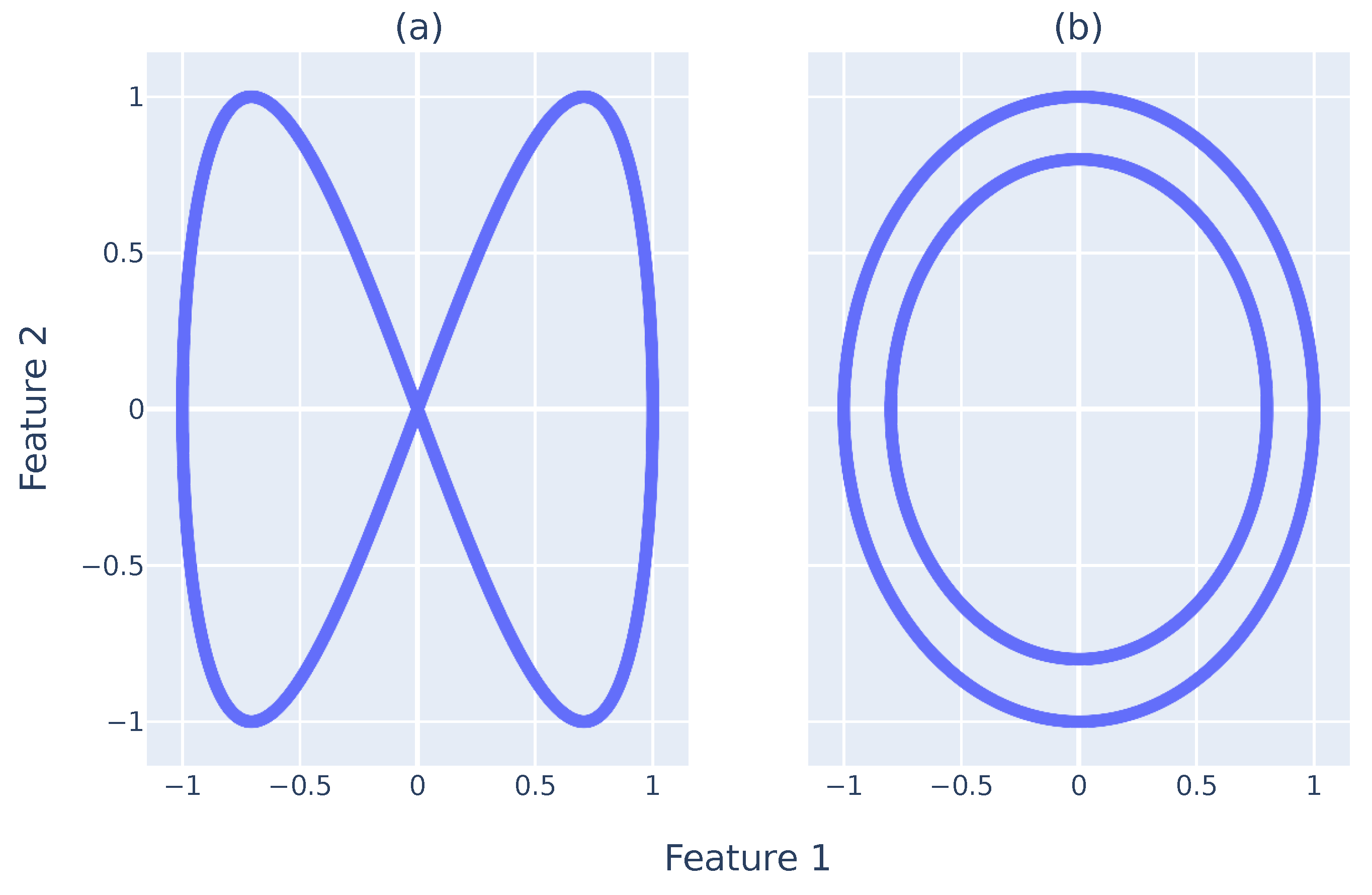
Figure 4a,b illustrates the point clouds,
, used to test the methodology followed and deployed. The two-point clouds have two dimensions,
, and have distinct shapes for easy visual guidance and explanation. The first
is shaped as an infinity sign, and the other forms two circles inside the other. Each
has 2000 data points. In this design, the
are considerably condensed. Therefore, performing an
analysis in both would create a
with all simplicial complexes dying at distances of close to 0, because a small
r creates connections between all points.
If one could perform the analysis, one would obtain two main topological features. However, one would die much earlier. This topological feature would represent the gap between circles in the two circles’ datasets. The inside circle would have its topological feature, which would persist for an extended period of time, r. In the infinity sign, there would be two topological features that would be born and die at the same time. Nevertheless, performing an analysis directly in an RSES is expensive and does not fit its constraints.
Our previous work [
14] showed that most RSESs can only handle
analysis using point clouds with 32 samples or less. Therefore,
had to be resampled into subdatasets of 32 samples for our case scenario. As shown in the next section, this resampling process will create a more meaningful
analysis, because points are expected to spread across feature space.
The two were divided into smaller point clouds, , one for training and the other for testing, to conduct the tests discussed in this work. Each X was composed of 1000 points. Each X was subdivided into five smaller point clouds of 200 points each, .
Five devices, called -devices, were then subdivided for training and five, called -devices, were used for testing. The and -devices were used to analyze a , where is the infinity-sign-shaped point cloud. Ten devices were considered for the analysis of the two circle-shaped . These devices were named -devices, and these simulated devices that would collect the wrong data in a real-life scenario.
All devices performed multiple analyses in random batches of 32 points. Then, the devices obtained the mean of each batch each time point. At each step, one of the 32 points was randomly replaced by a new one from the 200 available from . This test was intended to show that, independently of the starting point and given enough time, the mean landscape for both devices will converge to the same values. Therefore, performing a landscape analysis on-the-fly is possible, and one can verify the stability across multiple devices using this method.
One can obtain the landscape of each of the -devices, , and all -devices are expected to have similar landscapes. After verifying that the landscapes are similar, by plotting them, the method calculates the distance between the training landscapes’ means () and between each training landscape, ). Then the limit to accept another landscape as being from the original can be found, and this limit is called . Therefore, if , it is verified that a new device is collecting the same data as previously seen.
Now, one can calculate the -devices’ landscapes, . Then, one can verify whether . If the condition is true, . The training and testing landscapes are expected to be similar and close together. The same is done to the -devices, and it is expected that in most calculations one will obtain .
5. Results
The following section describes the results obtained from the tests made. The section is divided into three parts. The first regards the proof that, given enough landscapes, their mean will converge to a single shape. The second tries to show that the distance between the mean of all training landscapes is smaller for the training and testing datasets and much higher for the dataset. The third focuses on verifying how well our method can predict whether a given subsample of the point cloud is from the original dataset.
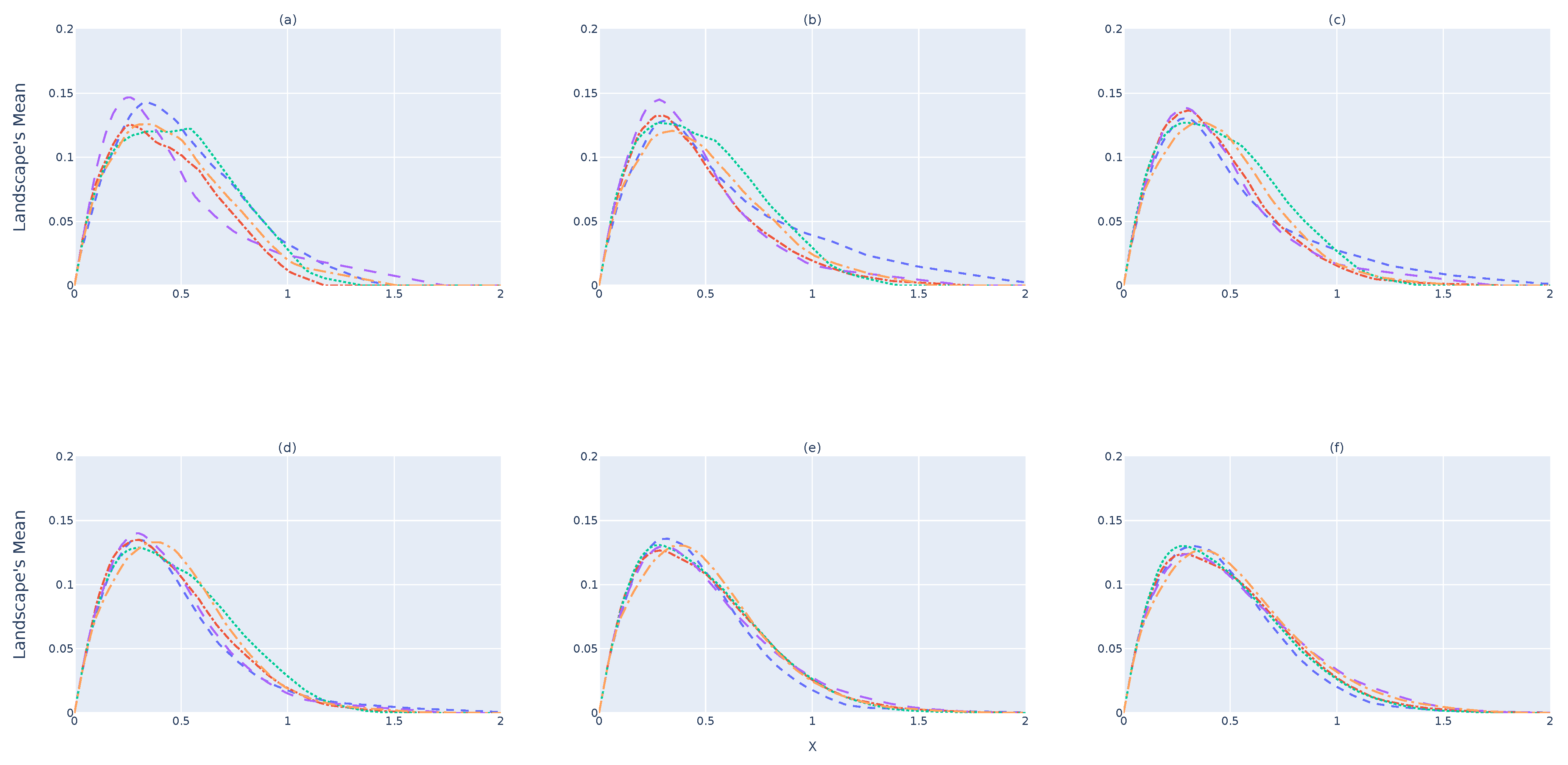
5.1. Convergence between Devices and Datasets
Figure 5a illustrates the
for
-devices when a single landscape is considered. It is expected that the amount of information provided from a single landscape will not represent the dataset, because the number of samples selected is small due to the memory constraints of an RSES. As shown,
values do not yet converge to the same shape. By increasing the number of landscapes to obtain
,
Figure 5b,c, shows better convergence to a single line. This convergence happens when 32 barcodes/landscapes are considered for
, as illustrated in
Figure 5d. Nevertheless, considering more landscapes, as shown in
Figure 5e,f, makes the results for each device almost indistinguishable. These results show that a single landscape does not provide enough information to verify whether the data collected follow the same
structure. One should consider and study the minimum number of landscapes to use before stating that
.
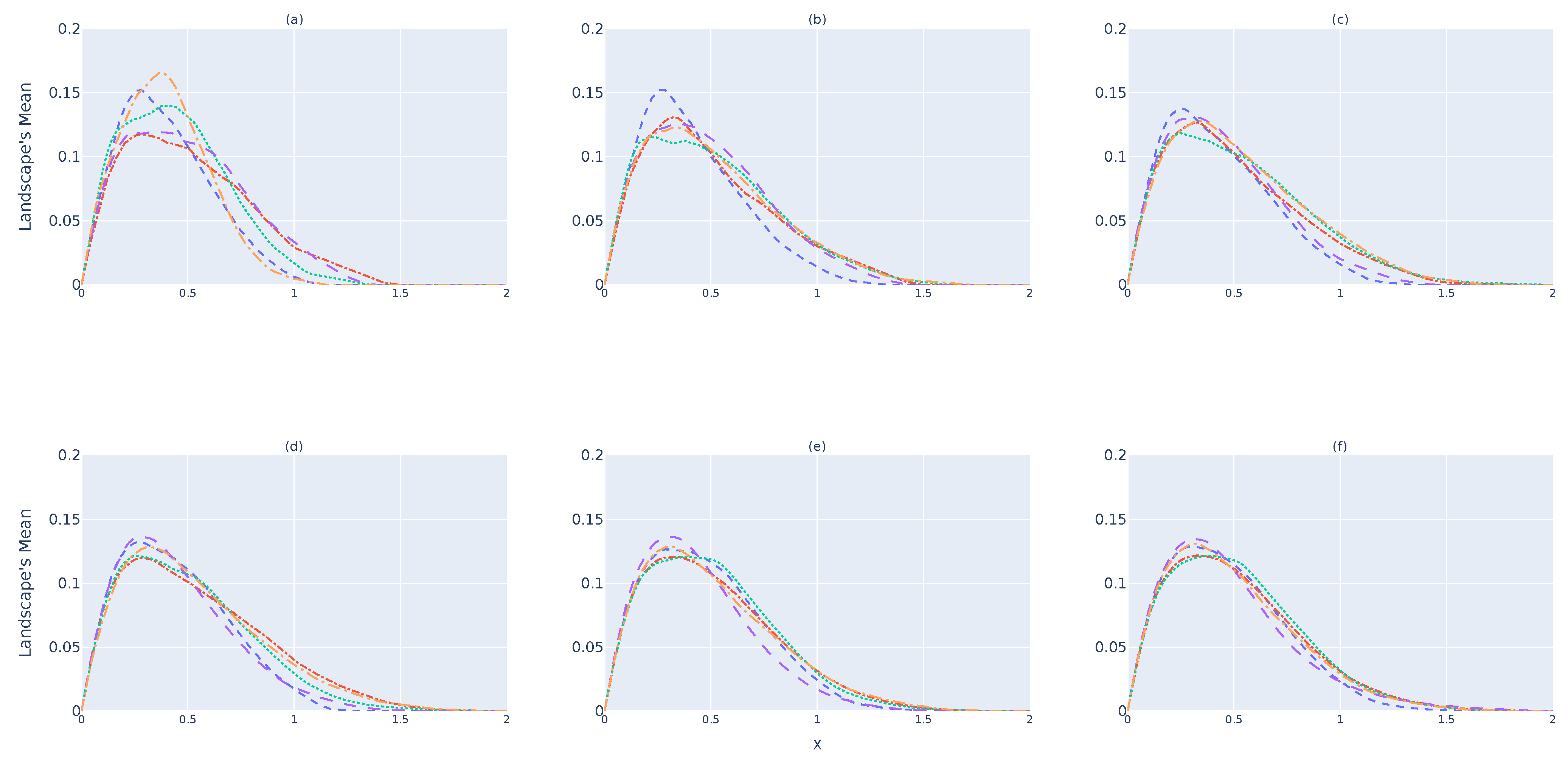
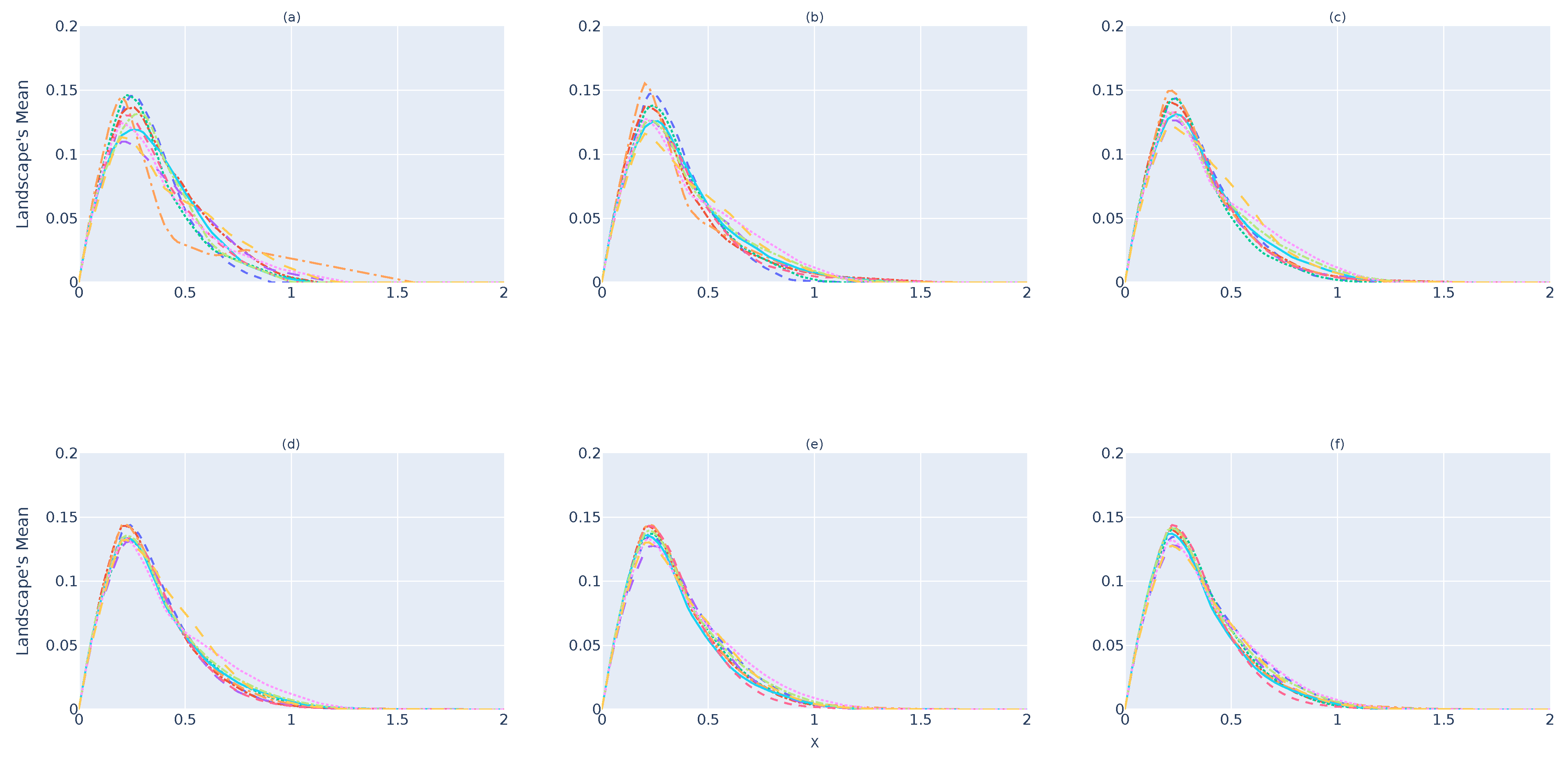
Figure 6 and
Figure 7 illustrate the results for the
and
devices, respectively. As it is possible to state, the same behavior as that verified for the
device occurs in both cases. By comparing
Figure 5,
Figure 6 and
Figure 7, one can perceive that
and
tend to be much more similar than
, which shows that the system will be capable of predicting whether
is a subset of the original point cloud or not. However, as discussed previously, one can see that, over time (d), there are greater differences between
and
, while
and
present themselves to be closer to each other. Therefore, 32 landscapes seems to be the point from which one can have greater certainty regarding
.
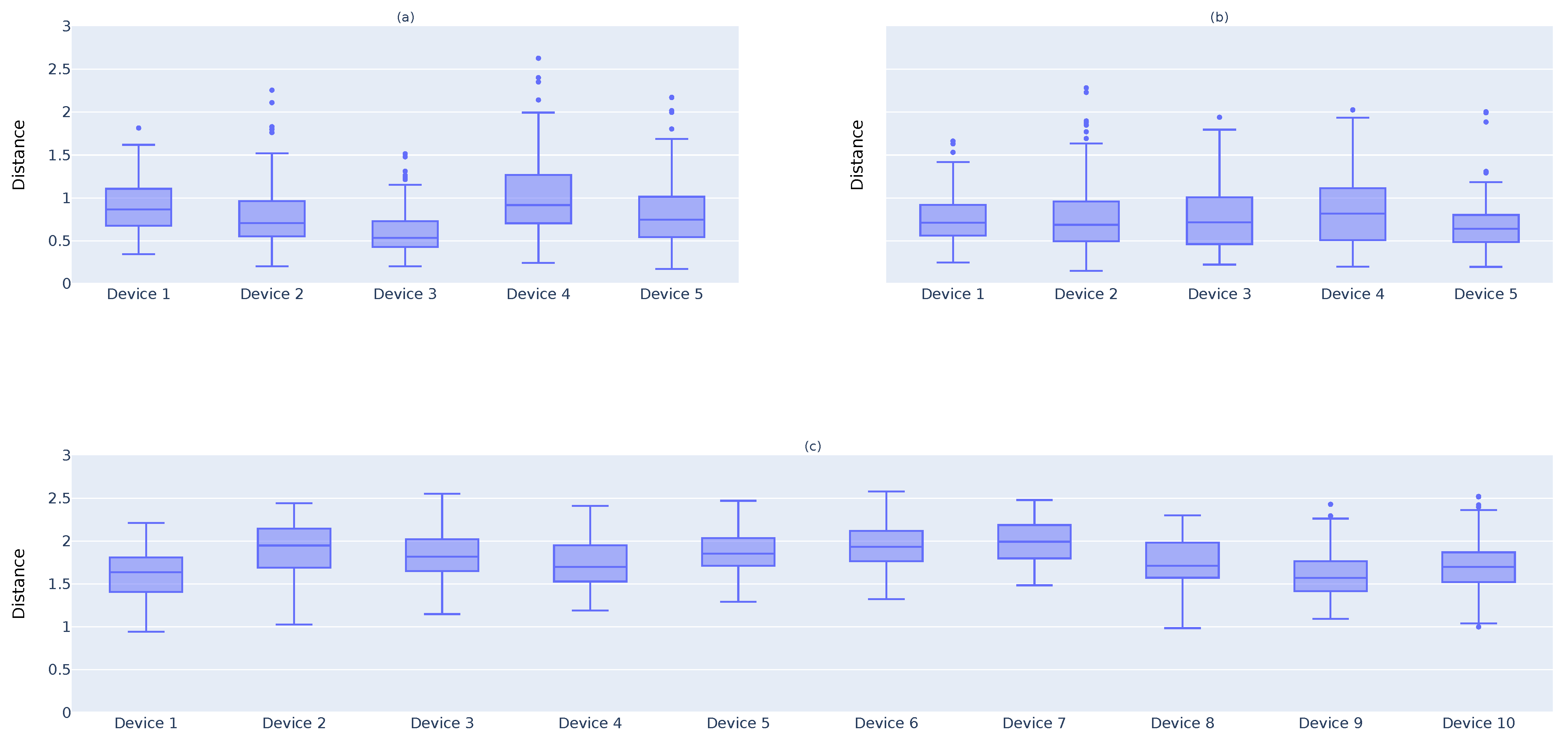
5.2. The Distance in Landscapes
Finding whether PLs are similar to , involves the use of a metric to measure the level of similarity and a threshold to accept or discard PLs as similar to . The threshold is the maximum distance value that separates the two datasets without creating significant number of false negatives. Finding the perfect threshold is essential to discard or avoid the acceptance of unwanted PLs. Therefore, depicting the results from the similarity metric between all PLs to is important to verify whether such a threshold exists and what its perfect value may be.
The second test was done to verify whether one can calculate the point-wise distance (
9) between all
and
values and, with it, calculate the perfect threshold,
, that will allow us to identify if
. The box plots in
Figure 8 show the
.
Figure 8a presents the distance results for the
devices. The box plot clearly shows that the majority of
values for these devices are under 1. Therefore, one may consider that the correct value is
. Now, one may look at
Figure 8b, which plots the distance for the
devices. Since these devices are collecting the same data as
, one must verify whether
is a suitable value to use for a threshold. As one can verify, the vast majority of
devices have
, which is a good result. Finally, one must verify whether the same
could discard the results from
devices.
Figure 8c shows that most
d values for
are above 1. Thus, if one selects
, the main intention to cut off the results from
devices is achieved.
5.3. Dataset Identification
The fundamental reasoning behind the entire work was to verify whether PL can be used to verify whether two devices are collecting the same dataset. If this occurs, one has achieved the goal of producing a system that can alert the device of malfunctioning or novel data findings. As shown in
Section 5.2, the threshold,
, is the perfect distance that most
and
values do not go above. Now, it is essential to verify, using random sampling and performing multiple tests, whether, with this
value, one can identify a landscape as not belonging to the infinity-shaped point cloud and determine which is the perfect number of landscapes to use to have certainty of such detection.
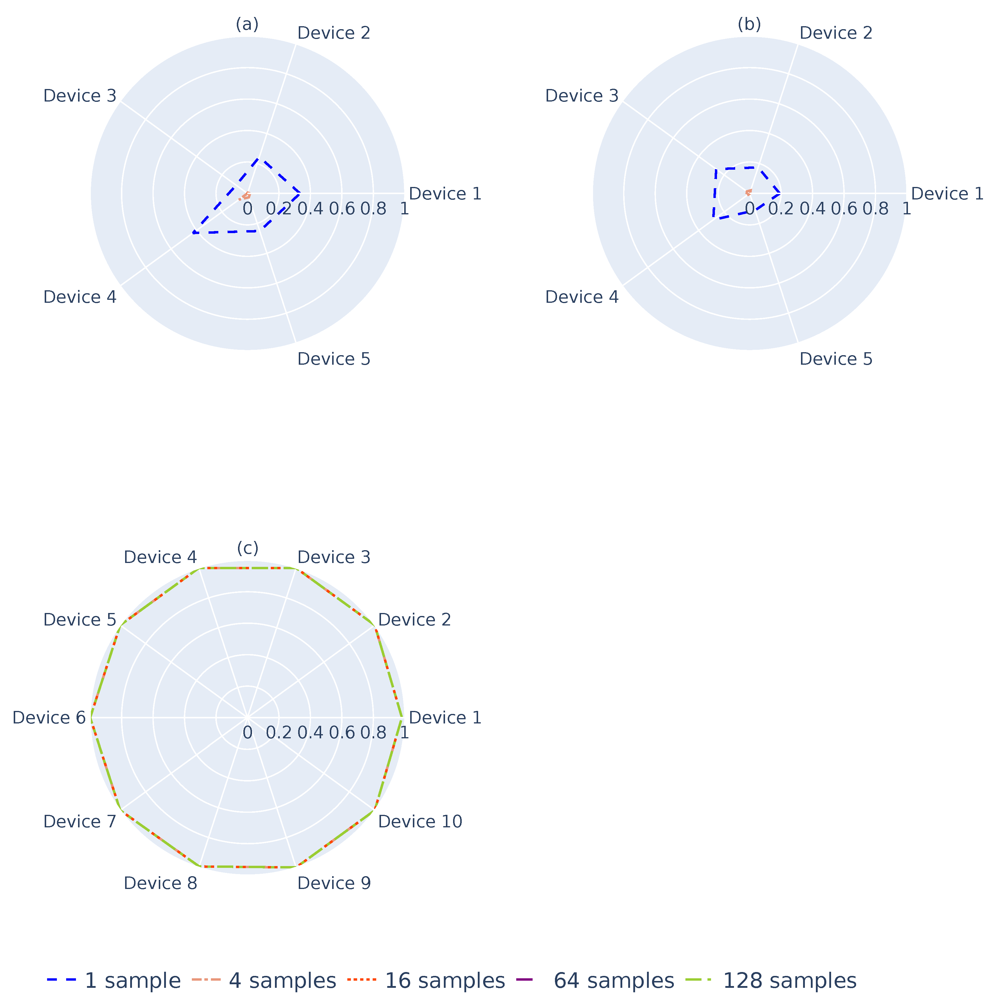
Figure 9 depicts the flag rate from generating 10,000 sampling groups from the previous landscapes obtained for each
. The groups were randomly generated and composed of 1, 4, 16, 64, or 128 landscapes. As one can see, using a single landscape (blue dashed line), the flag rates for both
and
-devices were high and in some cases were above 20%, as shown in
Figure 9a,b. For cases with 4 landscapes, the flag rate can be up to 5%, which is still a high result. With 16 landscapes, a residual number of landscapes was obtained for the flagged
and
devices, which is the expected behavior for the system. Contrary to this,
Figure 9c illustrates that, even with a single sample, the system can identify the
-devices. However, because of the flag rates of the
and
-devices, one must choose to use 16 or more landscapes for identification.
6. Conclusions and Future Work
The present work shows how Persistence Landscape analysis allows one to verify whether a given device collects data that are a subset of the original point cloud. Therefore, intelligent systems can now autonomously recognize when their performance may not be as expected, since the data collected do not represent the problem it was built from. Persistence Landscapes were obtained through H0 PD, which is computable in an RSES. With this analysis being made directly by an RSES, a new layer of trust is provided for intelligent systems built using these constrained devices. They can dynamically understand that they are facing an unknown environment, which is a stepping stone to avoiding errors, finding hardware malfunctions, and reducing the necessity for Cloud systems.
However, this method has some limitations, and the success of it is greatly dependent on the dataset and the proximity between the samples, because the 0-dimensional PH analysis constructs the PD based on connections, which means that if the points are close together, one will not have any meaningful information. Besides the intention to reduce the necessity for Cloud computing, this work could be improved with a central system or it could be used to decrease the workload of a Cloud system. For example, a device can initiate communication with a Cloud system only if it can previously verify that the point cloud being collected is not similar to any previous one seen. Moreover, if all devices send their PL to a Cloud system, even during data collection, the Cloud can check which devices should send data to avoid repetition.
In terms of future work, developments, and directions, the authors have considered the following: test the limits of this analysis with a broader range of datasets to verify whether there are any datasets for which this type of analysis will not provide meaningful results; test the differences in the PL analysis of -PD built with 32 samples or 64 samples; and create an algorithm to find the minimum number of landscapes to have certainty that .


 ,
, 


