
Rendezvous Based Adaptive Path Construction for Mobile Sink in WSNs Using Fuzzy Logic


Abstract
:1. Introduction
2. Related Work
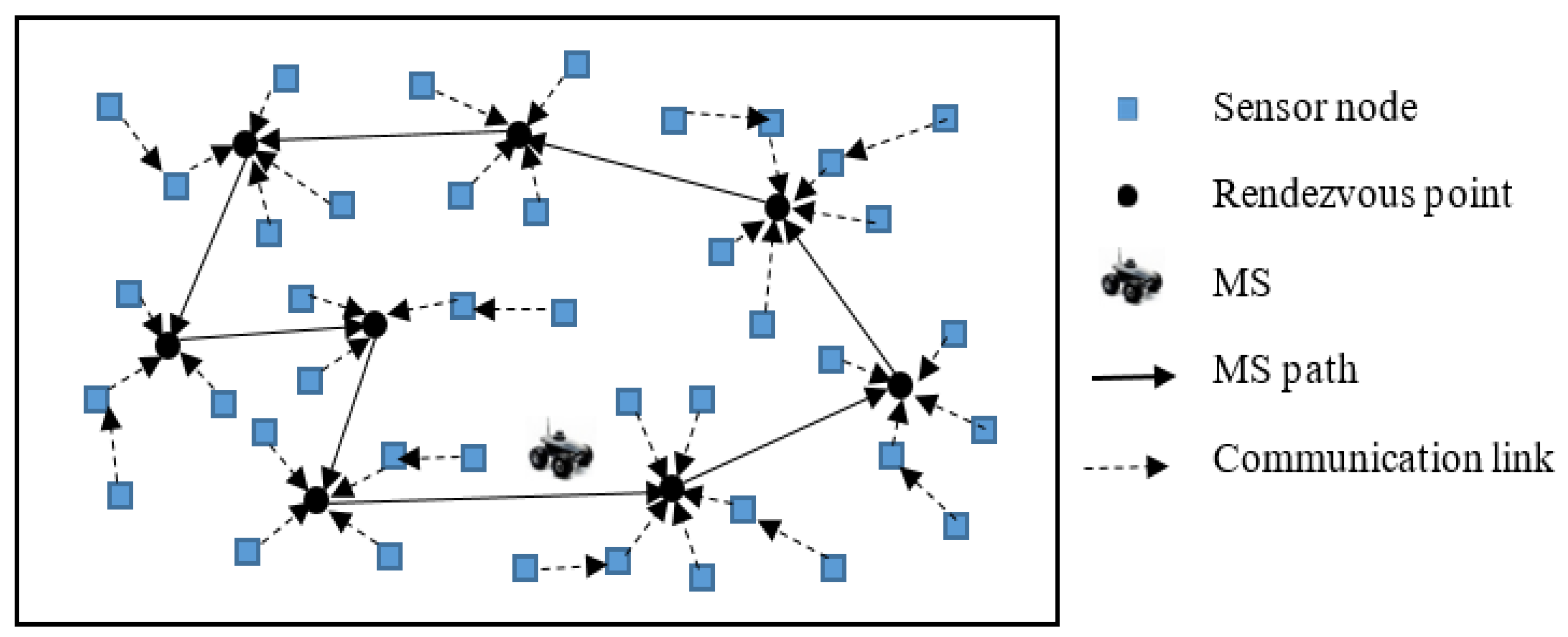
3. System Model
4. Proposed Approach
4.1. Initial Locations of the RPs
| Algorithm 1: Finding the initial locations of the RPs | |
| INPUT: S, PLthreshold | |
| OUTPUT: C, path for MS | |
| 1: | Begin RPs INITIAL LOCATIONS |
| 2: | P = k-means(S); // Cluster the S sensor nodes into P clusters using k-means algorithm [21] |
| 3: | for i = 1 to P do |
| 4: | Calculate the priority value of RP i using Equation (4) |
| 5: | End for |
| 6: | Sort the set P of RPs based on their priority values in descending order |
| 7: | C = { }; /* Set C contains the RPs that will be used to construct the MS path*/ |
| 8: | RPx = remove RP from P |
| 9: | |
| 10: | c = 1 |
| 11: | While True do |
| 12: | RPy = remove RP from P |
| 13: | |
| 14 | c = c + 1 |
| 15: | PL = TSP(C);/* Call traveling sales person algorithm to obtain the path between the RPs in C */ |
| 16: | If then break |
| 17: | End While |
| 18: | If (size(P) > 0) then /* if some RPs in P are not used to construct the path */ Redistribute the nodes attached to the RPs in P to the RPs in C |
| 19: | until the path length is equal or larger than the specified threshold. |
| 20: | End if |
| 21: | End |
- The current locations of the RPs.
- The ID of the corresponding RP for each sensor.
- The distance between each sensor and the corresponding RP.
- The energy level of each sensor.
- The number of surrounding sensor nodes for each sensor node.
4.2. Updating the RPs Locations
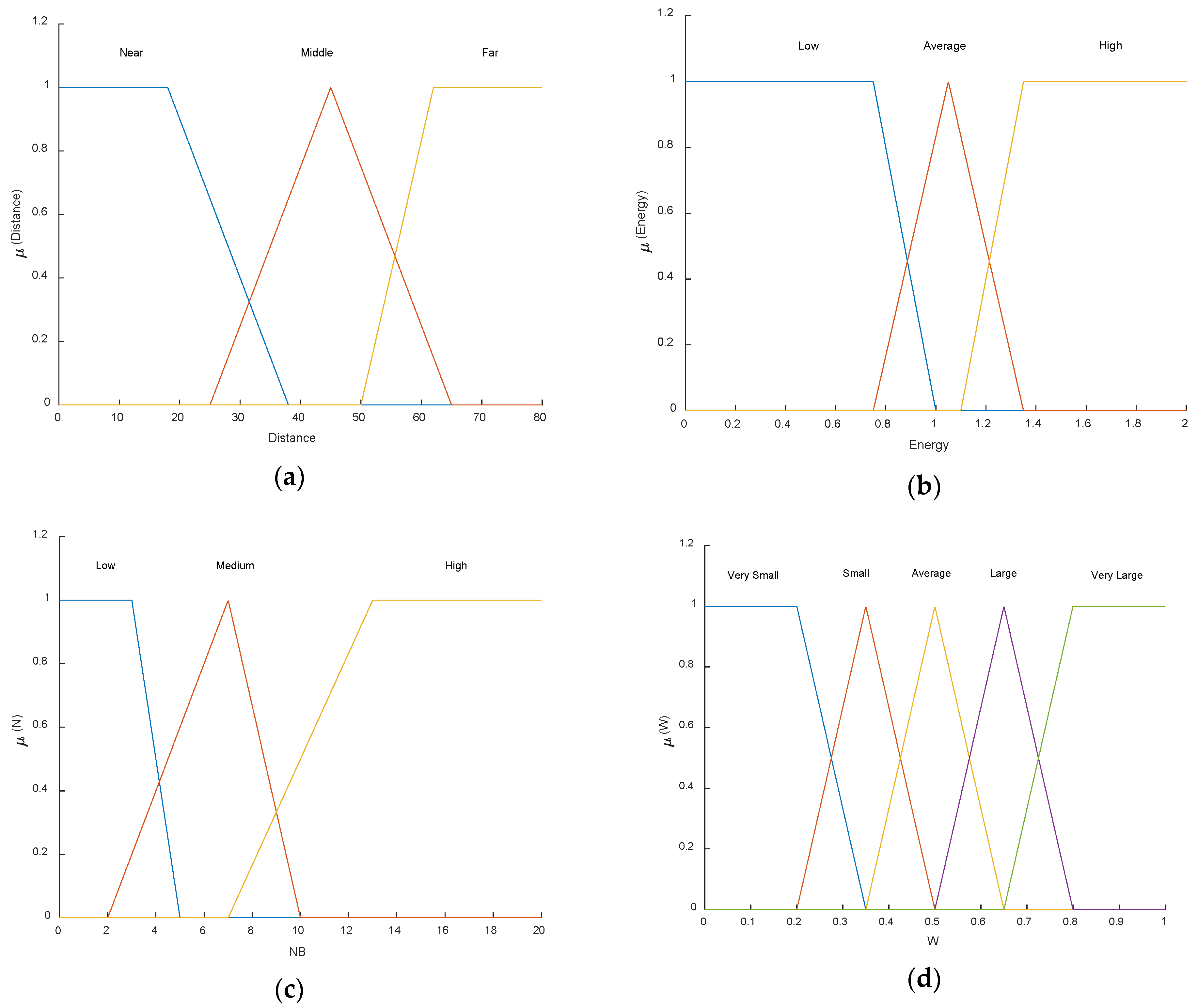
- The energy of each sensor around the RP. The energy level of each sensor influences how much the RP should be moved close to the sensor node. To balance the energy consumption and extend the network lifetime, the sensor with a low energy level has more impact to change the RP location and bring the RP close to it.
- The distance between the sensor node and the corresponding RP. As the distance of transmission influences the amount of energy consumption, the location of RP should be updated to balance the distance between all sensor nodes and their corresponding RP. This factor has a significant impact to mitigate the overall energy consumption during the network lifetime.
- The number of sensor nodes around each node. The sensor node within the dense region has more impact compared to the sensor node within the sparse region to influence the change of the RP location. The idea behind this factor is to attract the MS towards the dense region in order to be close to as many nodes as possible and therefore reduce the energy that will be used for transmission by the sensor nodes. This factor breaks the tie when two or more nodes have the same distance to their corresponding RP. For example, when two sensors have the same energy level and the same distance from the current corresponding RP, the sensor node with a high number of surrounding sensor nodes will attract the MS to update the location of the current corresponding RP towards it more closely compared with the sensor node in the sparse region.
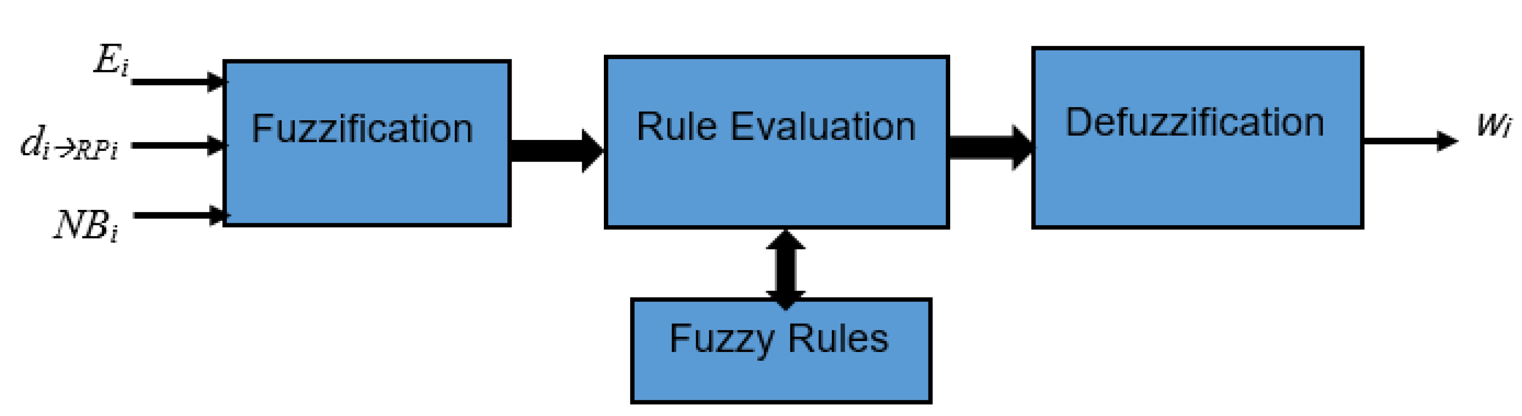
- Ei: the remaining energy of sensor node i.
- di⟶RPi: the distance between sensor node i and its corresponding RP.
- NBi: the 1-hop neighbors of sensor node i.
| Algorithm 2: Fuzzy-based Adaptive Path Selection | |
| INPUT: S, C, U /* U is the period value to update the path */ /* C is the set of RPs that are used to build the MS path */ /* S is the set of sensor nodes */ | |
| OUTPUT: updated path for MS | |
| 1: | Begin FUZZY_RPs |
| 2: | Round = 1; /* current round of collection data */ |
| 3: | while there is still active nodes AND (mod(Round, U) = 1) OR Round = 1) do |
| 4: | for j = 1 to sizeof(S) do |
| 5: | Determine the Nearest Corresponding RP of sensor sj |
| 6: | Discover number of the One-Hop nodes of sensor sj |
| 7: | End for |
| 8: | for i = 1 to sizeof(C) do |
| 9: | RPi = Ci |
| 10: | for each sensor sj associated with RPi do |
| 11: | wj =FIS [energy(sj), dist(sj to RPi), Num of one Hop nodes (sj) |
| 12: | Calculate XRPi→j using Equation (6) |
| 13: | Calculate YRPi→j using Equation (7) |
| 14: | End for |
| 15: | New X of RPi = Calculate New XRPi using Equation. (8) |
| 16: | New Y of RPi Calculate New YRPi using Equation (9) |
| 17: | End for |
| 18: | Round = Round + 1 |
| 19: | End while |
| 20: | Use TSP algorithm [25] to construct the path that passes through the RPs in C |
| 21: | End |
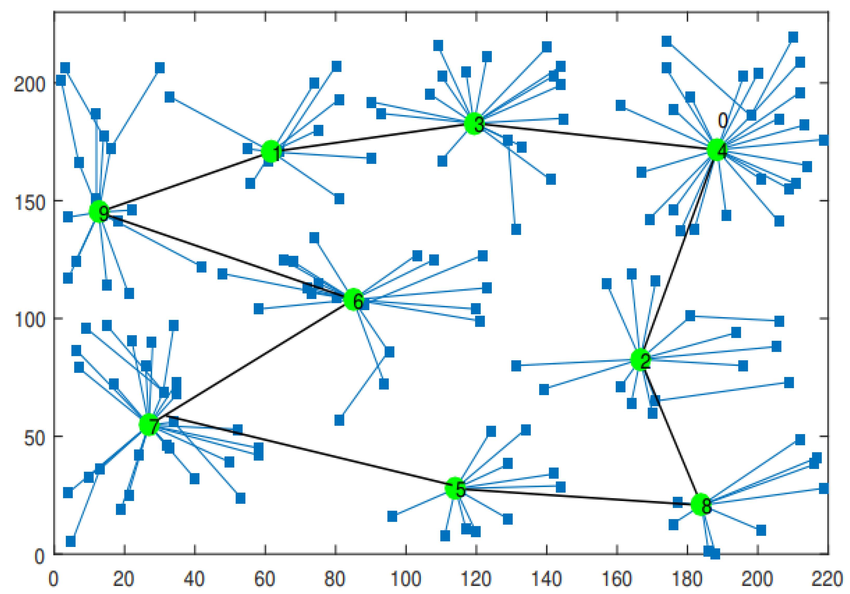
5. Performance Evaluation
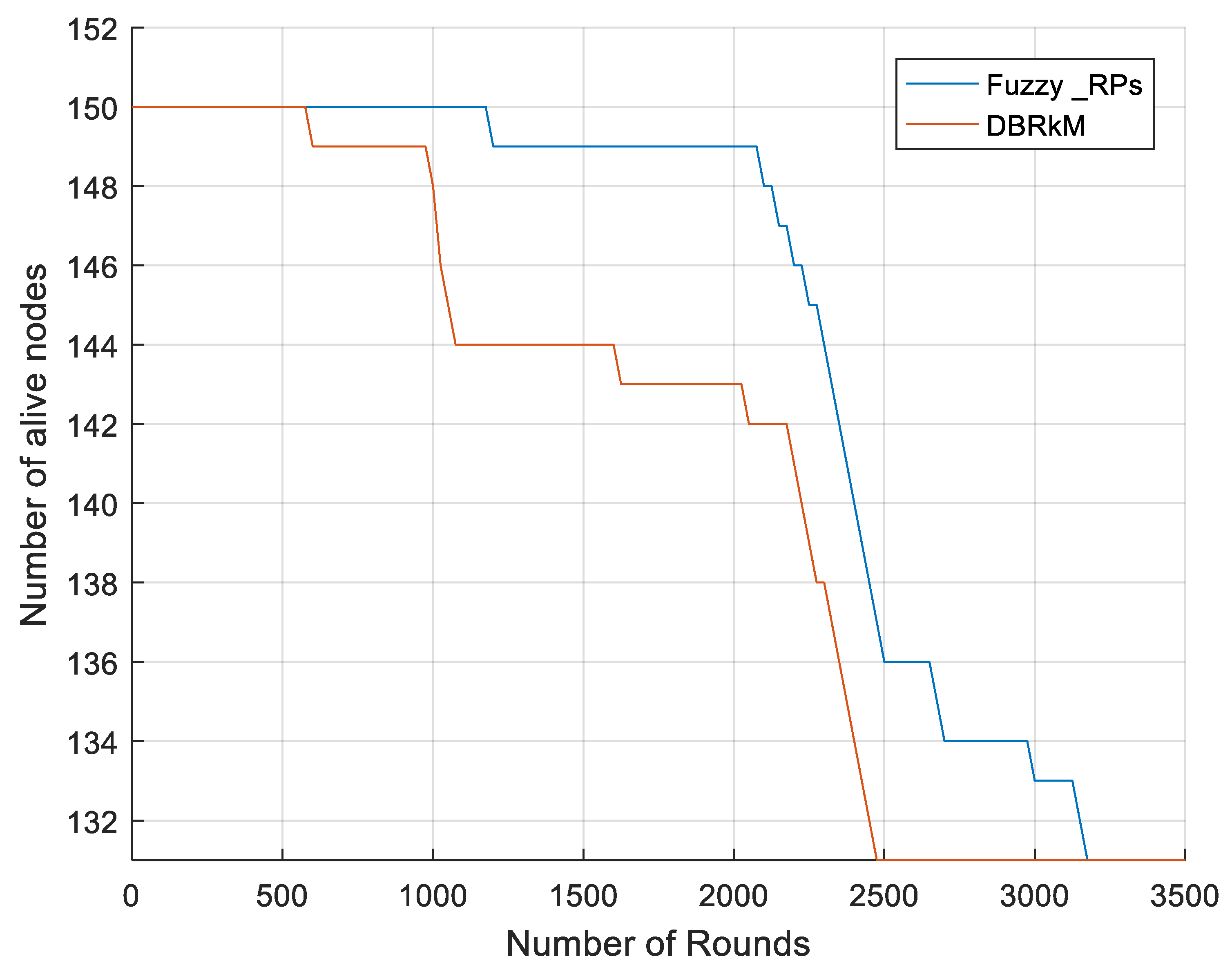
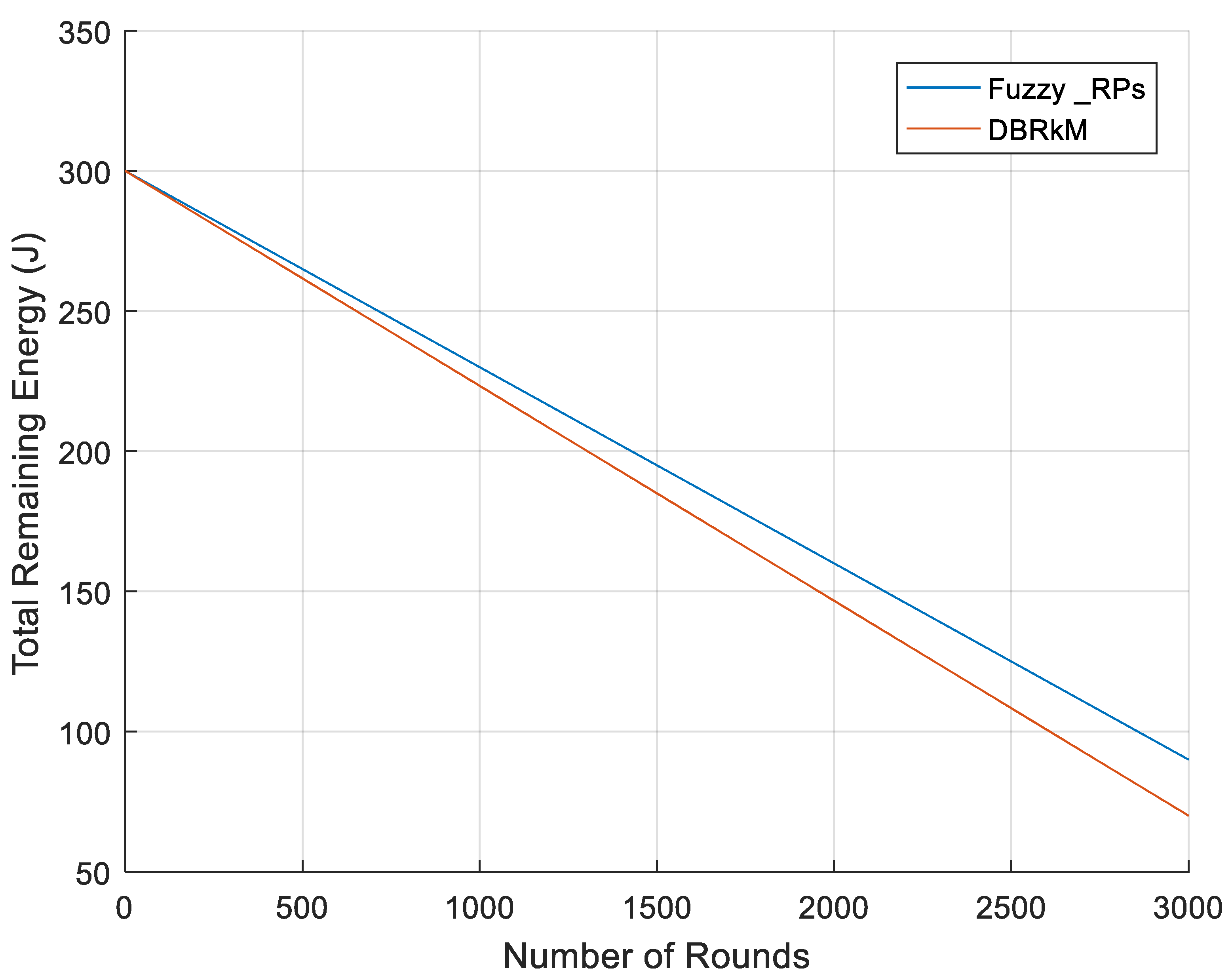
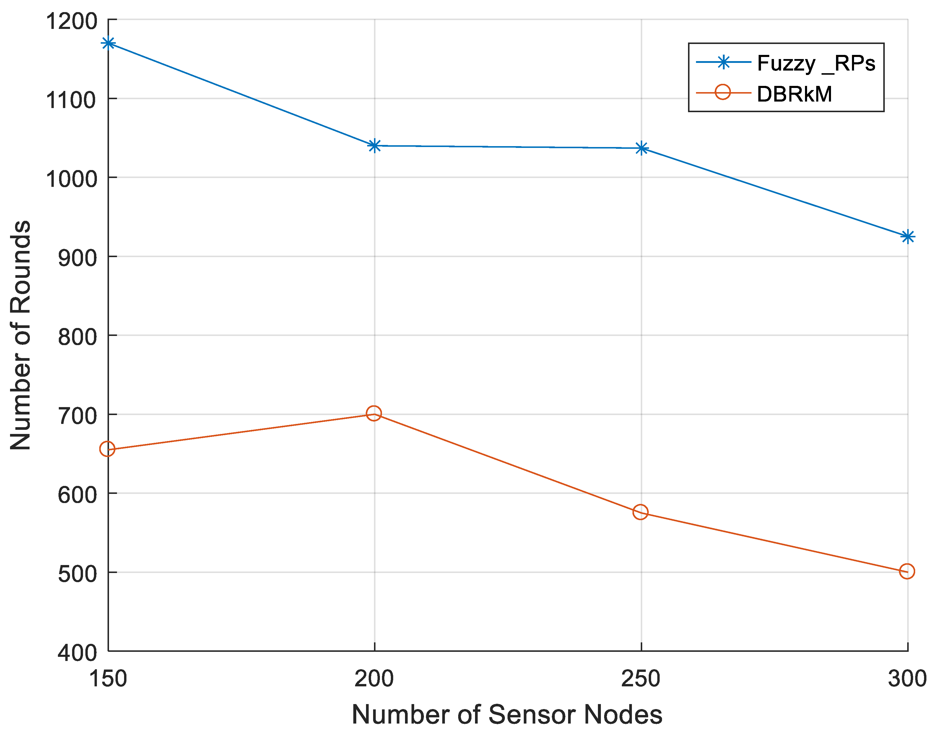
5.1. Network Lifetime
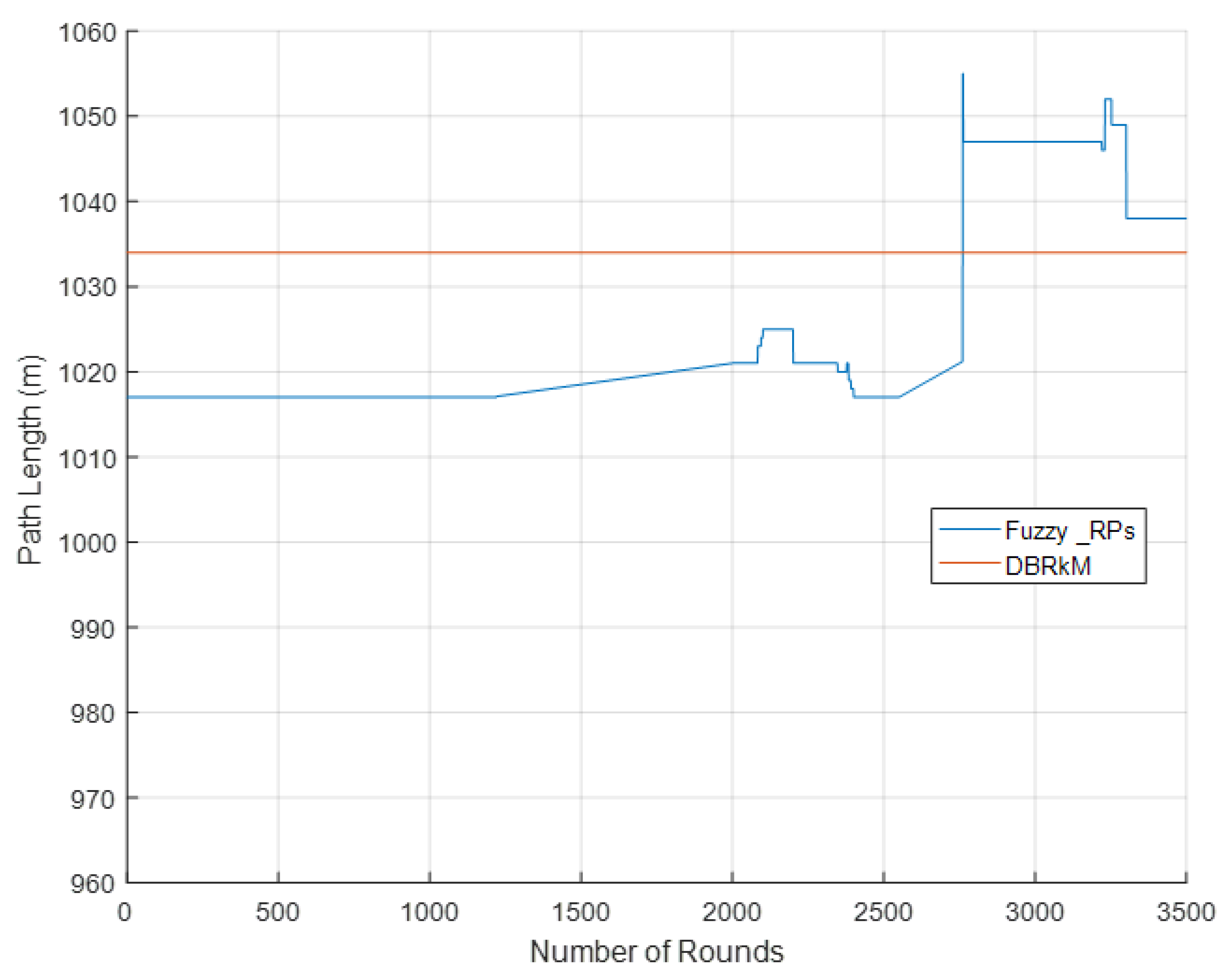
5.2. Path Length during the Network Life Time
6. Conclusions
Author Contributions
Funding
Informed Consent Statement
Data Availability Statement
Conflicts of Interest
References
- Abdur, R.M.; Arafatur, R.M.; Rahman, M.M.; Asyhari, A.; Bhuiyane, M.; Ramasamy, D. Evolution of IoT-enabled connectivity and applications in automotive industry: A review. Veh. Commun. 2021, 27, 100285. [Google Scholar] [CrossRef]
- Agarwal, V.; Tapaswi, S.; Chanak, P. A Survey on Path Planning Techniques for Mobile Sink in IoT-Enabled Wireless Sensor Networks. Wirel. Pers. Commun. 2021, 119, 211–238. [Google Scholar] [CrossRef]
- Akbar, M.; Javaid, N.; Abdul, W.; Ghouzali, S.; Khan, A.; Niaz, I.A.; Ilahi, M. Balanced Transmissions Based Trajectories of Mobile Sink in Homogeneous Wireless Sensor Networks. J. Sens. 2017, 2017, 4281597. Available online: https://www.hindawi.com/journals/js/2017/4281597/ (accessed on 1 September 2022). [CrossRef]
- Temene, N.; Sergiou, C.; Georgiou, C.; Vassiliou, V. A survey on mobility in wireless sensor networks. Ad Hoc Netw. 2022, 125, 102726. [Google Scholar] [CrossRef]
- Suh, B.; Berber, S. Rendezvous points and routing path-selection strategies for wireless sensor networks with mobile sink. Electron. Lett. 2016, 52, 167–169. [Google Scholar] [CrossRef]
- Gupta, P.; Tripathi, S.; Singh, S. Energy efficient rendezvous points based routing technique using multiple mobile sink in heterogeneous wireless sensor networks. Wirel. Netw. 2021, 27, 3733–3746. [Google Scholar] [CrossRef]
- Irish, A.E.; Terence, S.; Immaculate, J. Efficient data collection using dynamic mobile sink in wireless sensor network. In Wireless Communication Networks and Internet of Things, Lecture Notes in Electrical Engineering; Springer: Singapore, 2019; pp. 141–149. [Google Scholar] [CrossRef]
- Wang, J.; Gao, Y.; Yin, X.; Li, F.; Kim, H. An enhanced PEGASIS algorithm with mobile sink support for wireless sensor networks. Wirel. Commun. Mob. Comput. 2018, 2018, 9472075. [Google Scholar] [CrossRef] [Green Version]
- Liang, W.; Luo, J.; Xu, X. Prolonging network lifetime via a controlled mobile sink in wireless sensor networks. In Proceedings of the IEEE Global Telecommunications Conference (GLOBECOM), Miami, FL, USA, 6–10 December 2010; pp. 1–6. [Google Scholar] [CrossRef]
- Farzinvash, L.; Najjar-Ghabel, S.; Javadzadeh, T. A distributed and energy-efficient approach for collecting emergency data in wireless sensor networks with mobile sinks. AEU Int. J. Electron. Commun. 2019, 108, 79–86. [Google Scholar] [CrossRef]
- Park, J.; Moon, K.; Yoo, S.; Lee, S. Optimal stop points for data gathering in sensor networks with mobile sinks. Wirel. Sens. Netw. 2012, 4, 8–17. [Google Scholar] [CrossRef] [Green Version]
- Kaswan, A.; Nitesh, K.; Jana, P.K. Energy efficient path selection for mobile sink and data gathering in wireless sensor networks. AEU-Int. J. Electron. Commun. 2017, 73, 110–118. [Google Scholar] [CrossRef]
- Banimelhem, O.; Taqieddin, E.; Shatnawi, I. An Efficient Path Generation Algorithm Using Principle Component Analysis for Mobile Sinks in Wireless Sensor Networks. J. Sens. Actuator Netw. 2021, 10, 69. [Google Scholar] [CrossRef]
- Sharma, S.; Puthal, D.; Jena, S.K.; Zomaya, A.Y.; Ranjan, R. Rendezvous based routing protocol for wireless sensor networks with mobile sink. J. Supercomput. 2017, 73, 1168–1188. [Google Scholar] [CrossRef]
- Vajdi, A.; Zhang, G.; Zhou, J.; Wei, T.; Wang, Y.; Wang, T. A New Path-Constrained Rendezvous Planning Approach for Large-Scale Event-Driven Wireless Sensor Networks. Sensors 2018, 18, 1434. [Google Scholar] [CrossRef] [PubMed]
- Raj, P.V.P.; Khedr, A.M.; AL Aghbari, A. Data gathering via mobile sink in WSNs using game theory and enhanced ant colony optimization. Wirel. Netw. 2020, 26, 2983–2998. [Google Scholar] [CrossRef]
- Boyineni, S.; Kavitha, K.; Sreenivasulu, M. Mobile sink-based data collection in event-driven wireless sensor networks using a modified ant colony optimization. Phys. Commun. 2022, 52, 101600. [Google Scholar] [CrossRef]
- Donta, P.K.; Amgoth, T.; Annavarapu, C.S.R. An extended ACO-based mobile sink path determination in wireless sensor networks. J. Ambient Intell. Hum. Comput. 2021, 12, 8991–9006. [Google Scholar] [CrossRef]
- Ghaleb, M.; Subramaniam, S.; Ghaleb, S.M. An Adaptive Data Gathering Algorithm for Minimum Travel Route Planning in WSNs Based on Rendezvous Points. Symmetry 2019, 11, 1326. [Google Scholar] [CrossRef] [Green Version]
- Sun, G.; Liu, Y.; Zhang, J.; Wang, A.; Zhou, X. Node Selection Optimization for Collaborative Beamforming in Wireless Sensor Networks. Ad Hoc Netw. 2016, 37, 389–403. [Google Scholar] [CrossRef]
- Hartigan, J.A.; Wong, M.A. Algorithm as 136: A k-means clustering algorithm. Appl. Stat. 1979, 28, 100–108. [Google Scholar] [CrossRef]
- Zadeh, L.A. Fuzzy sets. Inf. Control 1965, 8, 338–353. [Google Scholar] [CrossRef] [Green Version]
- Heinzelman, W.R.; Chandrakasan, A.; Balakrishnan, H. Energy-efficient communication protocol for wireless micro sensor networks. In Proceedings of the 33rd Annual Hawaii International Conference on System Sciences, Maui, HI, USA, 7 January 2000; pp. 1–10. [Google Scholar] [CrossRef]
- Banimelhem, O.; Abu-hantash, A. Fuzzy logic-based clustering approach with mobile sink for WSNs. In Proceedings of the 13th International Computer Engineering Conference (ICENCO), Cairo, Egypt, 27–28 December 2017. [Google Scholar] [CrossRef]
- Johnson, D.S.; McGeoch, L.A. Experimental analysis of heuristics for the STSP. In The Traveling Salesman Problem and Its Variations; Springer: Boston, MA, USA, 2007; pp. 369–443. [Google Scholar] [CrossRef]


| Term | Definition |
|---|---|
| S | Set of sensor nodes |
| si | Sensor node i |
| Sj | Set of sensor nodes associated with RP j |
| P | Set of potential RPs |
| C | Set of RPs that are used to build the MS path |
| SRP(i) | Number of sensor nodes associated with RP i |
| HRP(i) | Average hop distance between RP i and the sensor nodes associated with it |
| (XRPi, YRPi) | Location of RPi |
| Ei | Remaining energy of sensor node i |
| di⟶RPi | The distance between sensor node i and its corresponding RP |
| NBi | The 1-hop neighbors of sensor node i |
| PL | Path length |
| v | MS speed |
| Rule Number | Inputs | Output w | ||
|---|---|---|---|---|
| Distance | Energy | Number of Neighbors | ||
| 1 | Near | Low | Low | Average |
| 2 | Near | Low | Average | Large |
| 3 | Near | Low | High | Very Large |
| 4 | Middle | Low | Low | Average |
| 5 | Middle | Low | Average | Large |
| 6 | Middle | Low | High | Very Large |
| 7 | Far | Low | Low | Large |
| 8 | Far | Low | Average | Very Large |
| 9 | Far | Low | High | Very Large |
| 10 | Near | Average | Low | Small |
| 11 | Near | Average | Average | Average |
| 12 | Near | Average | High | Large |
| 13 | Middle | Average | Low | Small |
| 14 | Middle | Average | Average | Average |
| 15 | Middle | Average | High | Very Large |
| 16 | Far | Average | Low | Average |
| 17 | Far | Average | Average | Large |
| 18 | Far | Average | High | Large |
| 19 | Near | High | Low | Very Small |
| 20 | Near | High | Average | Small |
| 21 | Near | High | High | Average |
| 22 | Middle | High | Low | Very Small |
| 23 | Middle | High | Average | Average |
| 24 | Middle | High | High | Small |
| 25 | Far | High | Low | Average |
| 26 | Far | High | Average | Large |
| 27 | Far | High | High | Large |
| Parameter | Value |
|---|---|
| Target Area | 220 × 220 m2 |
| Number of sensor nodes | 150–300 |
| Initial Energy of sensor nodes | 2 Joule |
| Communication Range (Rc) | 40 m |
| Packet Size (Kb) | 4000 bits |
| Speed of mobile sink (v) | 2 m/s |
| Eelect | 50 nJ/bit |
| Mp | 0.0013 pJ/bit/m4 |
| Number of Sensor Nodes | Number of Rounds until First Node Dies | Improvement (%) | |
|---|---|---|---|
| Fuzzzy_RPs Approach | DBRkM Approach | ||
| 150 | 1172 | 655 | 78.93 |
| 200 | 1044 | 704 | 48.30 |
| 250 | 1037 | 575 | 80.35 |
| 300 | 928 | 505 | 83.76 |
Disclaimer/Publisher’s Note: The statements, opinions and data contained in all publications are solely those of the individual author(s) and contributor(s) and not of MDPI and/or the editor(s). MDPI and/or the editor(s) disclaim responsibility for any injury to people or property resulting from any ideas, methods, instructions or products referred to in the content. |
© 2023 by the authors. Licensee MDPI, Basel, Switzerland. This article is an open access article distributed under the terms and conditions of the Creative Commons Attribution (CC BY) license (https://creativecommons.org/licenses/by/4.0/).
Share and Cite
Banimelhem, O.; Al-Quran, F. Rendezvous Based Adaptive Path Construction for Mobile Sink in WSNs Using Fuzzy Logic. Computers 2023, 12, 66. https://doi.org/10.3390/computers12030066
Banimelhem O, Al-Quran F. Rendezvous Based Adaptive Path Construction for Mobile Sink in WSNs Using Fuzzy Logic. Computers. 2023; 12(3):66. https://doi.org/10.3390/computers12030066
Chicago/Turabian StyleBanimelhem, Omar, and Fidaa Al-Quran. 2023. "Rendezvous Based Adaptive Path Construction for Mobile Sink in WSNs Using Fuzzy Logic" Computers 12, no. 3: 66. https://doi.org/10.3390/computers12030066