1. Introduction
Although intuitively understandable, the word epidemic can sometimes be complex to define. To help the research community solve this problem, O’Neil, E. A. and Naumova, E. N. [
1] published a research paper that elucidates the different definitions of this term. We have three definitions from [
1].
O’Neil, E. A. and Naumova, E. N. define an epidemic as “any increase in the incidence of a disease, to refer to even one case”. They call this definition the weakest. Another definition given to the epidemic by the authors is “any number of identified cases in a given space or time or taking both into account”. The third definition we will use here is “an increase in the occurrence of a disease in a defined population that is clearly greater than the usual or normal number observed in that population”.
The commonality of these three definitions and the popular and intuitive conception we may have of the epidemic is “the number of cases”. An epidemic is necessarily related to the number of people suffering from the disease [
2]. The greater the number, the greater the epidemic. The faster the epidemic spreads, the larger the number grows. This is why in the fight against an epidemic, the decrease in its spread is always the first battle [
3,
4]. For this reason, we decided to address this issue in this research work.
Indeed, the socio-health objective of this work is to propose an enriched Machine Learning (ML) model that will contribute to the fight against the spread of epidemics. To do this, we have set ourselves the goal that our model will be moderately better than the models existing in the literature regarding the detection of people with disease. It will not allow many of the positive cases to escape, which can infect others and increase the incidence of the epidemic.
The technical objective of this research work is to propose a Random Forest (RF) model with improved metrics compared to the default model. The choice of the Random Forest method is mainly based on our previous studies [
5,
6], which allowed us to identify Random Forest as one of the most suitable methods for epidemic prediction studies. We therefore decided to look into this method to propose a model. To ensure that our proposed RF model performs better than the default RF, we needed to test both models on the same data and variables. We will also needed to measure these two models with the same metrics to be able to compare the results.
To reach this goal, we first went through the literature to discover the work of other IT researchers in the fight against epidemics. The results of our findings are presented in
Section 2 of this article. Subsequently, we chose coronavirus disease 2019 (COVID-19) as the outbreak on which we will test our model. The description of the dataset, the ML models used to compare the performance of the model we propose, the evaluation criteria (metrics) used, and the research methodology are presented in
Section 3 of this article.
Section 4 presents the results obtained during the conduct of the research methodology. These results include data pretreatment, analysis and splitting, some algorithms including the one our model implements, the construction of our model, the results of the execution of our model taking into account each step of our algorithm, and the results of the evaluation of metrics compared to other models. It is in
Section 5 that we make an argument for the results presented in
Section 6. This discussion shows how our model manages to satisfy the socio-medical objective of this research. We start from an analysis of the metric values obtained by our model in comparison with other models to establish a link with the fight against the spread of the epidemic. The conclusion of this article is presented in
Section 6.
2. Related Work
The fight against the COVID-19 epidemic is challenging in many ways. Since the beginning of 2020, researchers around the world have tried to solve every aspect of this struggle. However, the primary goal of governments and leaders around the world in the fight against COVID-19 is to limit the spread of the disease. This is also stated by Ahamad M. M. et al. [
1].
Ahamad, M. M. et al. [
1] have implemented and applied models that predict and select the characteristics (variables) that correctly determine whether a person is positive or negative. In other words, these models allow researchers to determine the order of significance of the variables. Based on the variables and data on which [
1] applied these models, they obtained the following results: fever (41.1%), cough (30.3%), lung infection (13.1%), and runny nose (8.43%). [
7] conducted a study to predict the number of new people infected, dead, and recovered in the next ten days. The models developed by [
7] were built on the basis of four methods: Linear Regression (LR), Least Absolute Shrinkage and Selection Operator (LASSO), Support Vector Machine (SVM), and exponential smoothing (ES). The results obtained by the authors proved that the ES method is the best of the four, followed by LR, LASSO and SVM.
Greco, M. et al. [
8] conducted a study to predict the mortality rate of COVID-19 patients. The purpose of their study was to predict the outcome of the crisis in the intensive care unit. At the end of the study, they found that the following characteristics were strongly related to mortality: age, number of comorbidities, and male gender. Muhammad, L.J. et al. [
9] looked at predicting recovery of patients from COVID-19. They developed models with four algorithms. The model built with DT was better than the others with an accuracy of 99.85%. Narin, A. et al. [
10] have built a model based on CNN (Convolutional Neural Networks). The built model uses X-ray images to predict COVID-19 contamination at an early stage. Similarly, [
11] have proposed a model they named DarkCovidNet that predicts COVID-19 contamination from chest CT images.
In [
12], Mirri, S and co-authors developed a model that was used to predict the resurgence of corona virus in the nine provinces of Emilia-Romagna, during the period September–December 2020. The robustness of the model proposed in the work of Mirri, S et al. is based, among other things, on the fact that the model was trained with all the COVID-19 infections that occurred in the region concerned, the values of all the particles collected in the experimental period and the succession of restrictions imposed by the Italian government. The model proposed in [
12] obtained an accuracy of 90%.
The spread of the epidemic has also been studied by [
13]. In their work, they study the future expansion of COVID-19, the likely time when the epidemic will reach its peak, and the time when it may end. Yang, Z. et al. [
14] built a model to predict the peak and size of the epidemic in China. Dianbo, L. et al. [
15] developed a model for real-time prediction of the number of people living with COVID-19 in China. Remuzzi, A. and Remuzzi, G. [
16] conducted a study to predict the expansion of the epidemic in Italy and its impact in China. Studies such as [
17,
18] focused on real-time prediction of cases of COVID-19 contamination worldwide and early responses to these cases.
In other works, supervised Machine Learning models have been used to predict whether a person is COVID-19 positive or negative. These include the work of [
19,
20]. In [
9], the authors used a Mexican dataset that included age, sex, pneumonia, diabetes, asthma, hypertension, cardiovascular disease, obesity, chronic kidney disease, tobacco, and outcome (COVID-19 results). To make the prediction, the authors used and evaluated the following models: Decision Tree (DT), Logistic Regression (LR), Naive Bayes (NB), Support Vector Machine (SVM), and Artificial Neural Network (ANN). They came to the following conclusion: DT proved to be the best model in terms of the ’Accuracy’ metric with 94.99%; LR (94.41%), NB (94.36%), SVM (92.40%), and ANN (89.20) follow-up; while for ‘sensitivity’ metric, SVM takes the first place with 93.34%, ANN (92.40%), DT (89.20%), LR (86.34%), and NB (83.76%); and finally on the “specificity” metric, the first position is held by NB with 94.30% followed by DT (93.22%), LR (87.34%), ANN (83.30%), and SVM (76.50%). Although all models share the top spot in this study, we can easily see that on average the DT model comes in first with 92.47% followed by NB with 90.81%, LR with 89.36%, ANN with 88, 30%, and finally SVM with 87.41%.
Researchers used a publicly available dataset in [
20] to evaluate variables such as country, age, gender, fever, body-pain, runny nose, difficulty breathing, nasal congestion, sore throat, severity, and contact with COVID-19 patients. Their study included models such as GNB (Gaussian Naive Bayes), LR (Logistic Regression), SVM (Support Vector Machine), KNN (K-Nearest Neighbor), and DT (Decision Tree). Based on the authors’ evaluation of the four metrics Accuracy, Precision, Recall, and F1 score, DT performs the best on all the metrics.
Considering the above, it is evident that the two studies we cited, [
9,
20], all placed DT at the top of the list of models that best predict epidemics, and in particular, when it comes to determining whether patients have a positive or negative COVID-19 status. These studies are a strong support for the empirical demonstration of the study [
6] that we published in January 2021. This study was a brief literature review that took into account four epidemics: African Swine Fever (ASF), dengue, influenza, and oyster norovirus. At the end of that study, Random Forests distinguished itself from the others as being the best classifier in the prediction of epidemics followed by ANN (Artificial Neural Network).
At the time of this study, we based ourselves on the following works: [
21,
22,
23]. Each of these three works, in different contexts, came to the conclusion that Random Forests was the best classifier. Tapak L. et al. made a comparison of three ML methods (SVM, ANN, and RF) to judge their ability in predicting epidemics. They concluded that the temporal prediction of RF is better than that of the other methods studied (ANN and SVM) for such problems while ANN is better in detecting epidemics. Liang and co-authors tested and compared six ML methods (Bayes Net, ANN, SVM, AdaBoost, C4.5, and RF) based on four well-known comparison measures: SN (sensitivity), SP (specificity), ACC (Accuracy), and MCC (Matthew Correlation Coefficient) before opting for the RF to carry out predictive analysis of the epidemic of Swine Fever in Africa, because the result of this comparison placed the RF above others. Ducharme G. R. compared six methods (Bn, RLog, SVM, RF, KNN, and ANN). At the end of his study, Ducharme G. R. comes to the following conclusion: “The classifier that emerges from this exercise with the best scores is RF and its variants”.
This time, the fact that DT is aligned in first position in [
9,
20] knowing that RF is an improvement of DT because RF is a set of Decision Trees, is an additional evidence of the predictive quality of RF in the case of epidemics.
To this end, this study aims to propose a Random Forest model that performs better than the default model. We will use four metrics (Precision, Accuracy, F1Score, and Recall) to compare the two models. The study by Buvana and Muthumayil will allow us to compare the two models to other ML models implemented on the same data and variables for a fair comparison.
3. Materials and Methods
In this section, we will present and explain the data, Machine Learning (ML) methods, metrics, and the workflow we followed in this study, as well as other tools.
3.1. Dataset Description
The data we used comes from a publicly accessible dataset on GitHub [
24]. This dataset has already been used previously by other researchers including Buvana, M. and Muthumayil, K. in [
20]. The credibility of this study [
20] increased through its publication on the World Health Organization’s website [
25]. This dataset was built and put online by Simran Pandey [
26], researcher and member of the Industrial Design Cent (IDC) research center of the Indian Institute of Technology (IIT Bombay).
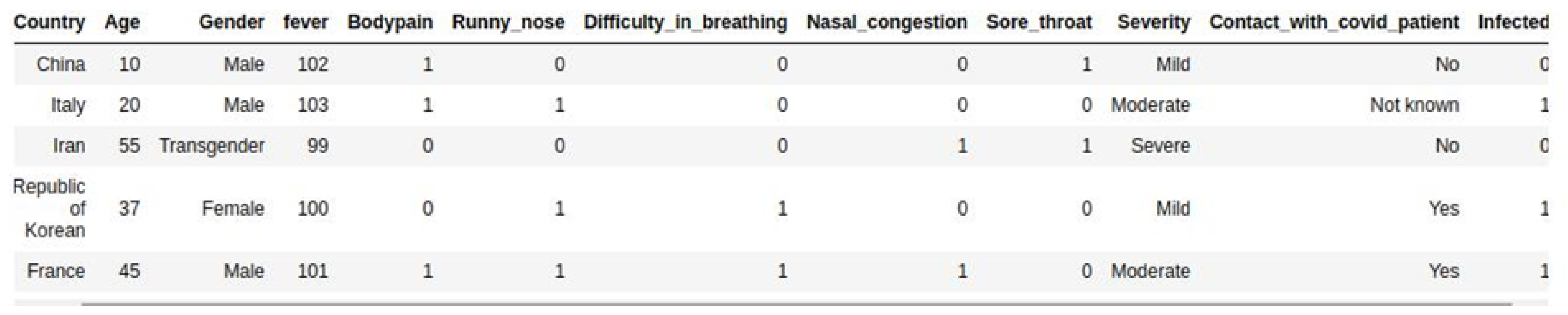
It also contains demographic and clinical data divided into twelve variables including: Country, Age, Gender, Fever, Bodypain, Runny_nose, Difficult_in_breathing, Nasal_congestion, Sore_throat, Severity, Contact_with_covid_patient, and Infected as well as 2500 entries. These data cover about 2500 persons.
3.2. Machine Learning Methods
This article aims to make a contribution to settling a problem that readily classifies itself in the supervised classification category. We begin by specifying that to solve a problem, supervised learning is used when the historical input/output data are known. The system is first trained with this data and then used to find outputs for new inputs [
27]. The problem is said to be classification when the variable to be predicted is a categorical variable. Our problem fully meets these criteria. Included in our 30,000 points of data is the variable “Infected”, which is the variable that this study is trying to predict. This is a categorical variable that determines whether a person is positive or negative.
On this basis, we turned to supervised Machine Learning (ML) methods that can do classification. The models developed in this study were built on the basis of the following six ML methods: GNB (Gaussian Naive Bayes), LR (Logistic Regression), SVM (Support Vector Machine), KNN (K-Nearest Neighbor), DT (Decision Tree), and RF (Random Forests).
3.2.1. Gaussian Naive Bayes
Gaussian Naive Bayes is a variant of Naive Bayes based on Bayes’ theorem. Bayes’ theorem makes it possible to find the conditional probabilities of occurrence of two events on the basis of the probabilities of occurrence of each event by following this formula:
With:
P(A/B) = The probability that event A is true knowing that B is true.
P(B/A) = The probability that event B is true knowing that A is true.
P(A) = The probability that A is true.
P(B) = The probability that B is true.
When Gaussian Naive Bayes is used for classification cases based on several variables, as is the case for us, a strong assumption is made: the variables are considered independent of each other [
28].
3.2.2. Logistic Regression
Logistic Regression is a static method often used for classification and predictive analysis [
29,
30]. Its algorithm is based on independent variables to predict the probability that an event may occur. Since prediction is a probability, it is between 0 and 1. For a binary classification, when the result is less than 0.5, the prediction will be 0; otherwise it will be 1 [
31].
To achieve the desired result, the logistic regression algorithm applies a transformation known as log odds. This logistical transformation follows these next mathematical formulas:
With:
Logit(pi): The target variable also called dependent variable.
X: The independent variable.
Beta: A coefficient estimated thanks to the maximum likelihood (MLE).
3.2.3. Support Vector Machine
Support Vector Machine (SVM) is used for both classification and regression but also for anomaly detection [
32]. In our case, as in most cases, it is used for classification. The SVM algorithm treats the dataset as a set of points and aims to find the optimal hyperplane that divides this set into two groups (two classes) in the case of a binary classification, such as ours. The challenge is to find, among so many possible hyperplanes, the one that best divides the two classes so that the class boundary is as far away as possible from the data points. It will therefore be a question of maximizing the margin [
33]. The margin is defined as the distance between the nearest data point and the hyperplane.
3.2.4. K-Nearest Neighbor
K-Nearest Neighbor (k-NN) is a nonparametric supervised classifier. It can be used for classification cases but also for regression cases although the latter use is infrequent. For the classification k-NN works on the assumption that similar points can end up next to each other. Based on this hypothesis a label is assigned to a point according to whether it is the majority around it.
3.2.5. Decision Tree
Decision tree (DT) is a non-parametric supervised classifier that can be used for classification and regression. Decision trees are built following the strategy “divide and conquer” from a dataset [
34]. This is because a Decision Tree is a hierarchical structure organized into three main elements: the root node, the inner node, and the leaf node.
Initially, all data is placed in the root node, which will then be divided into two or more nodes called internal nodes or decision nodes based on a rule [
35]. The internal nodes will in turn be divided to form others, and so on, recursively, until it is no longer possible to divide them. The last nodes are called leaf nodes; they are the final predictions.
For each node
S (internal or leaf), its estimate (label in the case of a classification) in relation to the target variable is calculated on the basis of entropy [
36,
37]:
With:
H(S): The entropy of node S. Determines the homogeneity of the node. The more it tends towards zero (0) the more homogeneous the node.
: The probability that an element of S is in class Ci.
3.2.6. Random Forest
Appeared in the 90s, Random Forest is a set method operating according to two basic principles: bagging and Random Feature Selection [
38,
39,
40]. Leo Breiman, in [
40], defines Random Forest as a classifier consisting of a set of elementary Decision Tree classifiers, denoted:
With:
: A family of independent and identically distributed random vectors, and within which each tree participates in the vote of the most popular class for an input data x.
Indeed, Random Forests benefits from the simplicity of Decision Trees while correcting their great weakness which is overfitting. This is an improvement to the Decision Trees. Random Forests has been designed to be more robust and accurate than a Decision Tree.
3.3. Evaluation Criteria
The objective of this article is to evaluate the performance of ML models in predicting epidemics for classification cases before proposing an enriched model. To achieve this end, we mainly considered four metrics: Accuracy, Precision, Recall, and F1 score, to evaluate six models: GNB, LR, SVM, KNN, DT, and RF. Subsequently, we considered the confusion matrix, in addition to the previous four metrics, to compare the default RF model and the proposed RF model. In the following, we will define the metrics used from an epidemiological perspective.
3.3.1. Accuracy
Accuracy is one of the most widely used metrics. It makes it possible to measure the accuracy of the model on all predictions. Indeed, accuracy is a measure of both the number of true positives and the number of true negatives. It can be used to measure simultaneously whether or not a prediction is correct [
41]. Its formula is as follows:
With:
TP (True Positive): Predictions that are positive and that are actually positive.
TN (True Negative): Predictions that are negative and that are actually negative.
FP (False Positive): Predictions that are positive but are actually negative.
FN (False Negative): Predictions that are negative but are actually positive.
3.3.2. Precision
Precision measures the number of people who are reported positive by the model and who are actually positive relative to the total number of people reported positive by the model [
41]. In other words, this metric allows us to estimate the degree of confidence we can have in a model’s predictions about a person’s likelihood of being infected. Its formula is as follows:
3.3.3. Recall
Furthermore, called Sensitivity, Recall is one of the essential metrics of the classification. It measures the number of people declared positive by the model and who are actually positive in relation to the total number of positive people in the dataset [
41,
42]. In other words, it is the metric that measures the model’s ability to detect all positive cases transmitted to it. It answers the following question: of all the positive records, how many were correctly predicted? A model with a high Recall will miss fewer positive cases. Its formula is as follows:
3.3.4. F1 Score
F1 Score also measures the performance of ML models. Indeed, F1 Score is the weighted average of Precision and Recall [
41]. F1 Score makes it possible to find the best compromise between Precision and Recall [
43]. Its formula is as follows:
3.3.5. Confusion Matrix
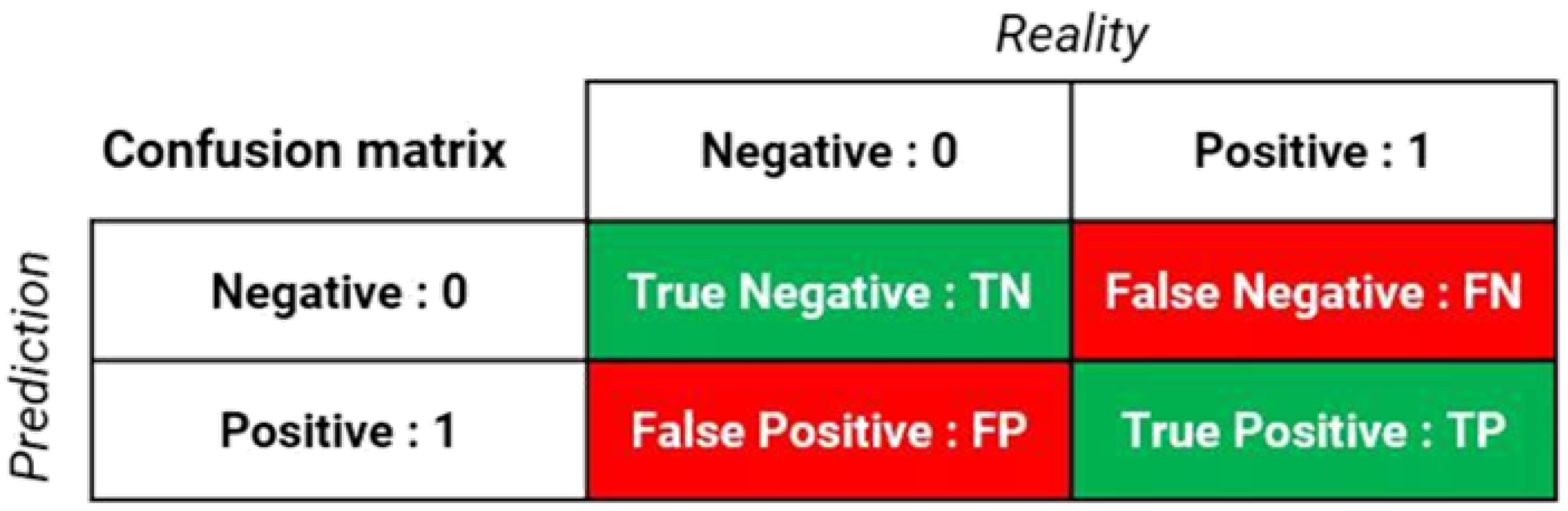
The confusion matrix or contingency table, shown in
Figure 1, is not a performance metric. On the other hand, it is a good way to visualize all the metrics previously defined.
A visual support (table) helps us observe how often predictions have been good compared to reality [
44]. The confusion matrix makes it possible to visualize directly on a table, for example, the number of correctly predicted positive people compared to the total number of predictions in the dataset. It will no longer be a question of measuring a metric (Accuracy, Recall, etc.) or the error rate, but rather of having precise figures related to the case treated [
44].
We used the confusion matrix in our case to visualize the result between the default RF model and the RF model we proposed.
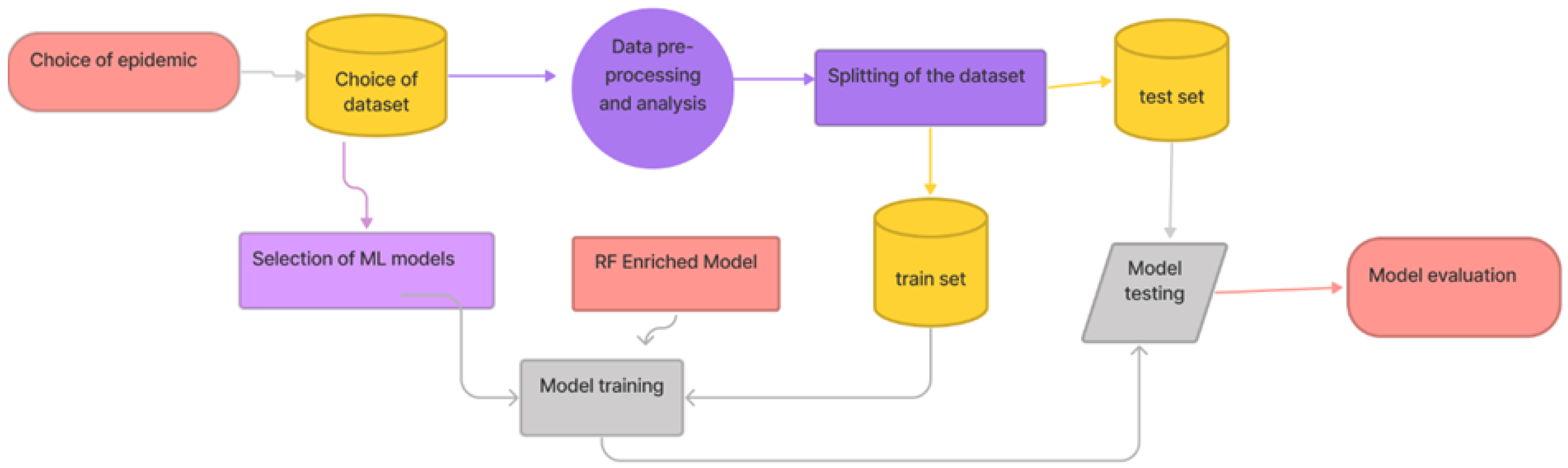
3.4. Research Methodology
Our research methodology is a nine-steps process:
Choice of epidemic: The question here is to determine which epidemic will serve as an example of experimentation.
Choice of dataset: After choosing the epidemic, it is then necessary to choose the dataset among those available in the literature. It is on this dataset that the proposed model will be tested.
Selection of ML models: To attest the performance of our model, it will be imperative to compare it to others.
RF Enriched Model: In this step, we will explain the process that led to the construction of our model.
Data pre-processing and analysis: This is the step that prepares the data to be used and then performs correlation studies to better understand our data before prediction.
Splitting of the dataset: Consists of dividing the dataset into two parts. One part for training and the other for testing.
Model training: This involves training all models, including the one that we proposed. Before that, the models to be used are selected, and the RF enriched model is proposed.
Model testing: This is about testing all models, including the one we offer.
Model evaluation: The aim here is to evaluate the models on the basis of the defined metrics.
4. Results
The purpose of this section is to present the results obtained after applying the research methodology summarized in
Figure 2. We recall that in this study, our main objective is to set up a classification algorithm based on Random Forests (Random Forests), to allow the COVID-19 test based on certain information provided by the patient to the AI (Artificial Intelligence) which will use it to predict the outcome. First, we will start with descriptive statistics on quantitative variables, we will conduct a correlation analysis between the variable of interest (target variable) and the other variables. Next, we will explain the basic algorithms of default Random Forests and the one we modified. Finally, we will develop a comparison between the models used by the reference article [
20], default RF, and our model that implements our algorithm.
4.1. Epidemic and Dataset
As a result of our need to respond to current realities and also to contribute to fight against COVID-19, we decided to take the COVID-19 pandemic as an example. For the choice of dataset we were driven by the following constraints:
A dataset built for a classification study;
All variables in the dataset must be collectible via a form (namely the ODK form [
45]);
The dataset must have been used in a scientific article;
The scientific paper using this dataset should include a comparison of several Machine Learning (ML) models based on the metrics cited in
Section 3.3;
At best, among the models compared in the article using this dataset, there must be Random Forests.
The outcome of our research led us to the dataset described in
Section 3.1 and whose header is represented in
Figure 3. All variables in this dataset can be collected via a form, it was used by Buvana, M. and Muthumayil K. in [
20]. From five previous constraints, this dataset fully fulfills the first four. For the fifth criterion (comparison of RF and other models), the presence of the DT (Decision Tree) model among the models compared in the article is sufficient to fill the RF gap because there is a clear link between RF and DT.
4.2. Data Pre-Processing, Analysis and Splitting
Analysis of data from our dataset reveals that we have a sample of people ranging in age from 10 to 89, as shown in
Figure 4. The average is 43 years and the median is 39 years. On the other hand, the majority of people belong to the 35–55 age group.
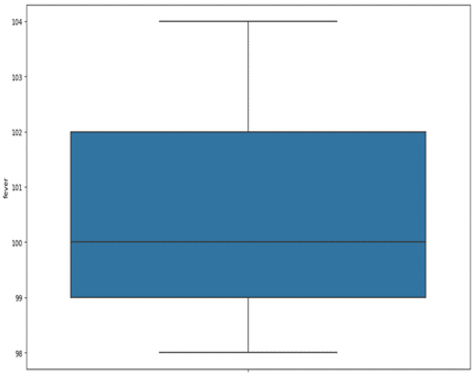
As for the body temperature of patients, it is expressed in Fahrenheit. It ranges from 98° to 104 °F, as shown in
Figure 5. The mean and median are about 100 °F with a standard deviation of 1.71. We observe that the majority of our subjects (between the first quartile and the third) have a temperature ranging between 99 °F to 102 °F (37.22 °C to 38.88 °C). Note that Celsius = (Fahrenheit-32)/1.8.
The correlation of the variable
Infected, the variable that determines whether a person is COVID positive or not, with the independent variables reveals interesting information. In
Table 1, that summarizes these correlations, it appears that the mode of transmission of COVID-19 is mainly through contact with a positive person with a correlation of 57%, and at the same time, it turns out that the patient who has not had contact with a positive person has 80% chance of being healthy.
The other two very influential characteristics are difficulty of breathing and sore throat which, if present, generally lead to a positive COVID test at 48.3% and 44.2% respectively. An abnormal fever is also an indicator leading to more than 39% of cases of the presence of the virus; this would justify taking temperatures in crowded places such as the bank or shopping mall, as it is one of the easy ways to detect suspected cases of COVID-19.
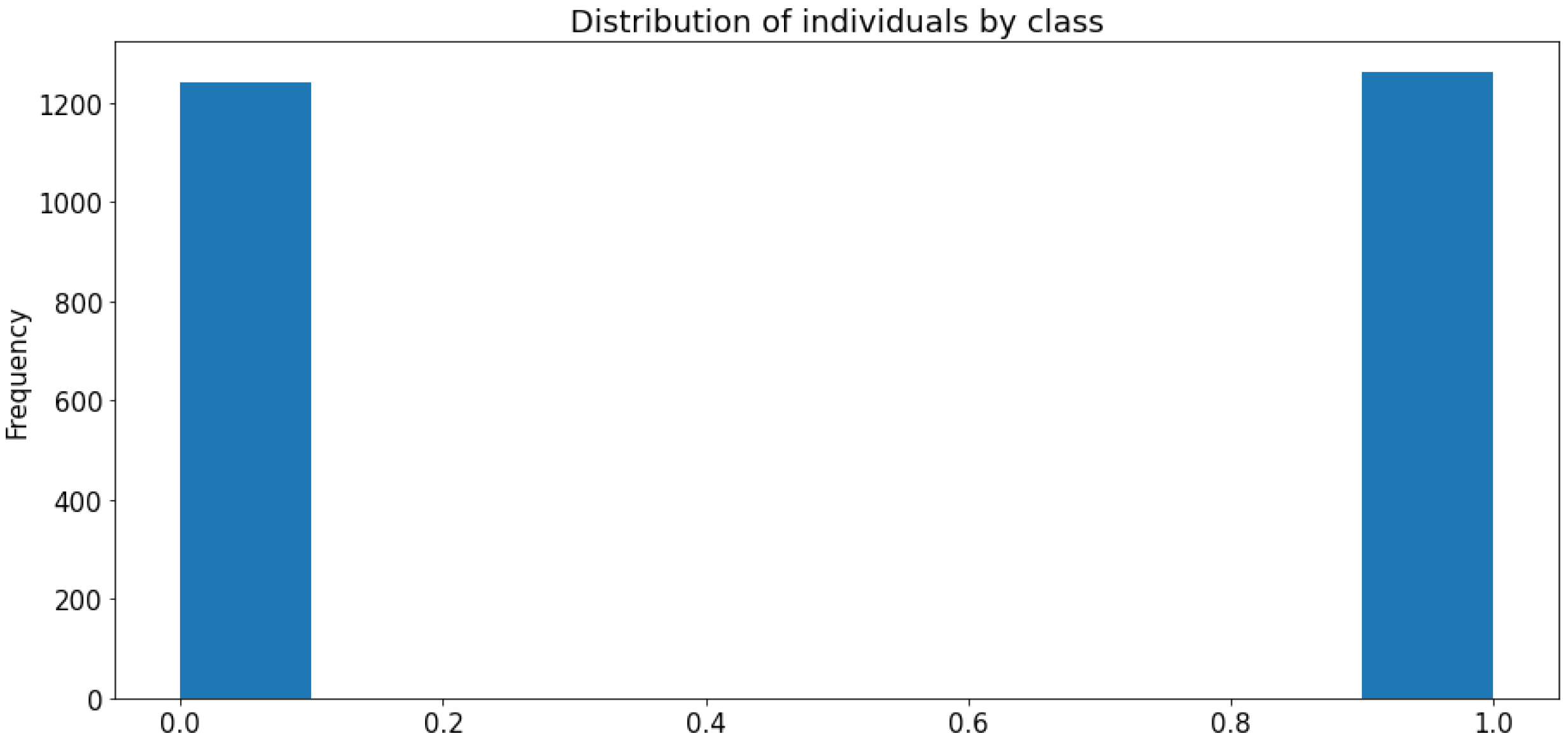
We look at the distribution of data according to two classes: positive (infected persons) represented by 1 and negative (healthy persons) represented by 0.
Figure 6 shows that the distribution is balanced by class thus avoiding bias caused by an over-representation of one class compared to the other causing a low accuracy rate of the model for the under-represented class. Before moving on to the implementation of our model, we had to adapt our data to the form understandable by our Machine Learning model, i.e., encoding. This dataset was well formatted and cleaned when it was downloaded, the majority of qualitative variables were already encoded.
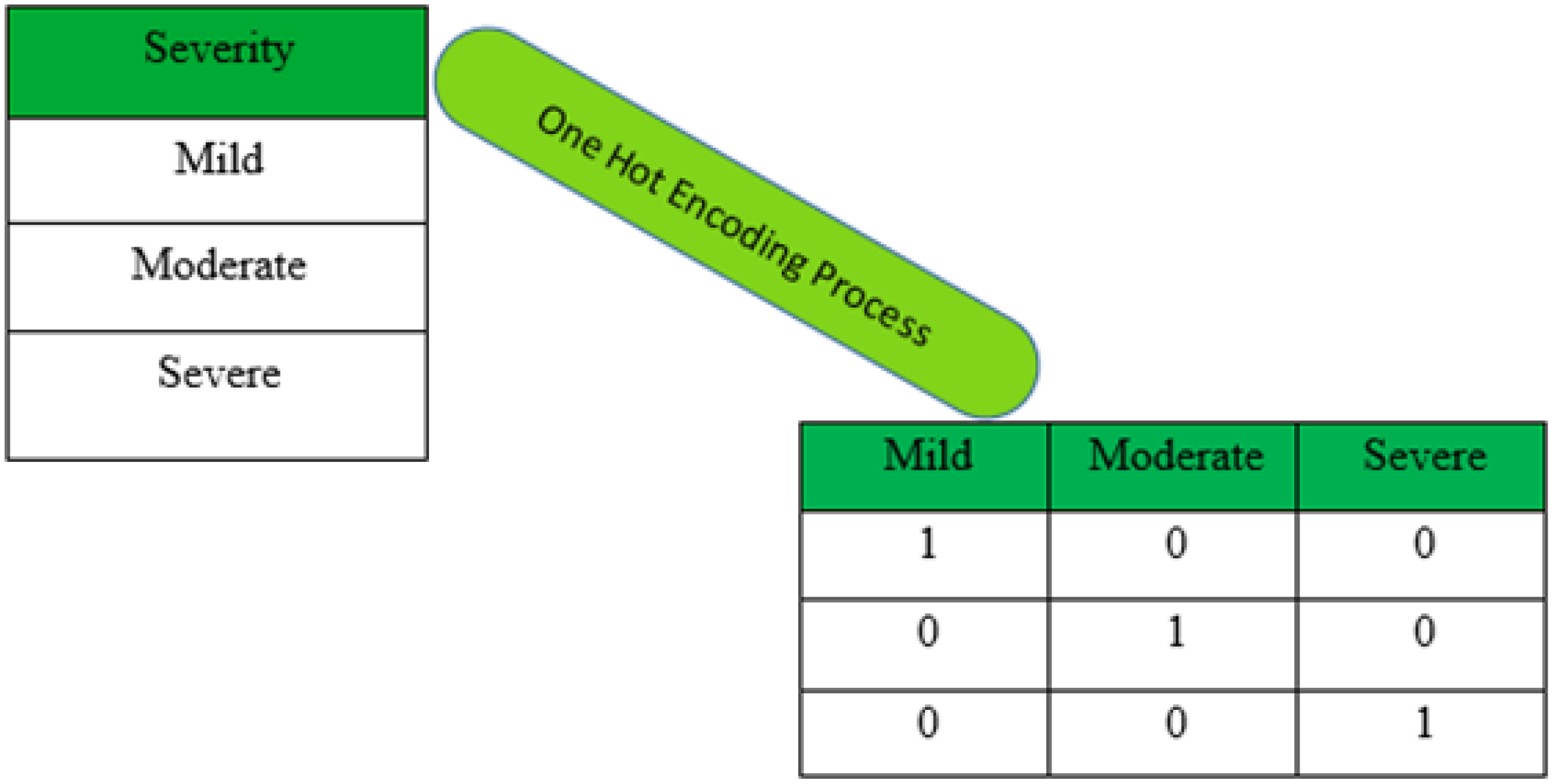
Thus, after data mining, we proceeded to code qualitative variables that were not yet encoded. To avoid scale effects for variables with more than two values, we opted for one-hot encoding, also called dummy encoding, allowing us to create a new indicator variable for each modality. This was the case for the variables “Severity” and “Contact_with_covid_patient”. The encoding took place as follows:
Gender: With 0/1 binary encoding for Male/Female.
Severity: The one hot encoding of this variable is shown in
Figure 7. It allowed to explode the variable in three: Severity_Moderate, Severity_Mild, and Severity_Severe. The three new variables were each binary coded: 0/1 for absence/presence.
Contact_with_covid_patient: The dummy encoding of this variable allowed to have three variables: Contact_with_covid_patient_yes, Contact_with_covid_patient_no, and Contact_with_covid_patient_ignore. The three new variables were each coded binary: 0/1 for absence/presence.
Other qualitative (or categorical) variables that were already encoded are: Bodypain, Runny_nose, Difficult_in_breathing, Nasal_congestion, Sore_throat, and Infected.
To train the model, we opted for data separation by adopting 80% to train the model and 20% to test the built model.
4.3. Model Training, Testing and Evaluation
As mentioned above, our study uses a dataset that was used by Buvana M. and Muthumayil K. in [
20]. We will base ourselves on the results they obtained for the first five models namely GNB, LR, SVM, KNN, and DT and then compare these results to what we obtained with default Random Forests and with Random Forests EP (Epidemiological Prediction) always on the same dataset.
Table 2 gives the results of metrics of six models, five of which came from the work of [
20] and the sixth from our work.
Here we call default RF, RF version presented by default in the scikit-learn package. Default RF is built on the basis of Forest RI algorithm proposed by Breiman L [
40] which uses the recursive Random Tree algorithm. Forest RI is considered as the reference algorithm of Random Forests [
46]. In order to propose an enriched RF model, which we have chosen to name RF EP, we have undertaken modifications into Forest RI. These changes led to a new algorithm we named Forests EP which uses the Var_Cust algorithm that we propose in addition to Random Tree used in Forest RI. It is on the basis of this algorithm that we built Random Forests EP. These Algorithms 1–4 and their explanations are given in the rest of this section.
| Algorithm 1 Forest RI |
| Input: T, the train set |
| Input: L, the number of trees in the forest |
| Input: K, the number of characteristics to be randomly selected at each node |
| Output: forest, all the trees that make up the built forest |
- 1:
for l from 1 to L do - 2:
Tl ← bootstrap set, whose data is randomly drawn (with delivery) from T - 3:
tree ← an empty tree, i.e., composed of its root only - 4:
tree.root ← RndTree(tree.root, , K) - 5:
forest ← forest ∪ tree - 6:
return forest
|
Forest RI explanation: It allows one to gather all the components of the Random Forests. With L the number of estimators to be used in forest construction, for each tree we use the RnTree construction method to construct the corresponding tree, using:
This operation makes it possible to create a tree at each iteration by ensuring the independence of opinion of these estimators. Finally, these trees are grouped together to constitute the so-called Random Forests because of the tree construction method.
| Algorithm 2 Random Tree |
| Input: n, the current node |
| Input: T, the set of data associated with node n |
| Input: K, the number of characteristics to be selected randomly at each node |
| Output: n, the same node, modified by the procedure |
- 1:
If n is not a leaf then - 2:
C ← K randomly selected characteristics - 3:
for everything A ∈ C to do - 4:
CART procedure for the creation and evaluation (Gini criterion) of the partition produced by A according to T - 5:
partition ← partition that optimizes the Gini criterion - 6:
n.addSons(partition) - 7:
for each son ∈ n.sonsNode do - 8:
RndTree(son, sons.done, K) - 9:
return n
|
Explanation of Random Tree: It allows for the establishment of a tree through the partitioning method based on the randomly chosen variables K. To build a child node (or potentially a sheet) from a node n, we apply the Gini criterion to each variable A ∈ C in order to choose the partition that minimizes the disorder, allowing us to predict the real value. This process is then used on each node to build the tree recursively.
| Algorithm 3 Forest EP |
| Input: X_train, the train set |
| Input: X_test, the test set |
| Input: y_train, training data label |
| Input: k, the number of variables to be eliminated from the learning set |
| Input: threshold_ratio, the amount of information to be retained in the training data |
| Input: L, the number of trees in the forest |
| Input: K, the number of characteristics to be randomly selected at each node |
| Output: forest, all the trees that make up the built forest |
- 1:
T_train_retain, T_test_retain = Var_Cust( X_train, X_test, y_train, n, threshold_ratio) - 2:
for l from 1 to L do - 3:
Tl ← bootstrap set, whose data are randomly drawn (with discount) from T_train_retains - 4:
tree ← an empty tree, i.e., composed of its root only - 5:
tree.root ← RndTree(tree.root, T l, K) - 6:
forest ← forest ∪ tree - 7:
return forest
|
| Algorithm 4 Var Cust |
| Output: n, the number of less significant variables to be removed from the database |
| Output: threshold_ratio, the amount of information to be kept in the main components |
| Output: X_train, train set before processing |
| Output: X_test, test set before processing |
| Output: y_train, training data label |
| Output: X_train_retain, train set after processing |
| Output: X_test_retain, test set after processing |
- 1:
T_train_retain, T_test_retain = Var_Cust( X_train, X_test, y_train, n, threshold_ratio) - 2:
for l from 1 to L do - 3:
Tl ← bootstrap set, whose data are randomly drawn (with discount) from T_train_retains - 4:
tree ← an empty tree, i.e., composed of its root only - 5:
tree.root ← RndTree(tree.root, T l, K) - 6:
forest ← forest ∪ tree - 7:
return forest
|
Explanation of Var_Cust algorithm when running the RF EP model:
(1): This step, shown in
Figure 8, extracts initial variables in the database that best explain the variable of interest (Infected), respecting the number n given as input.
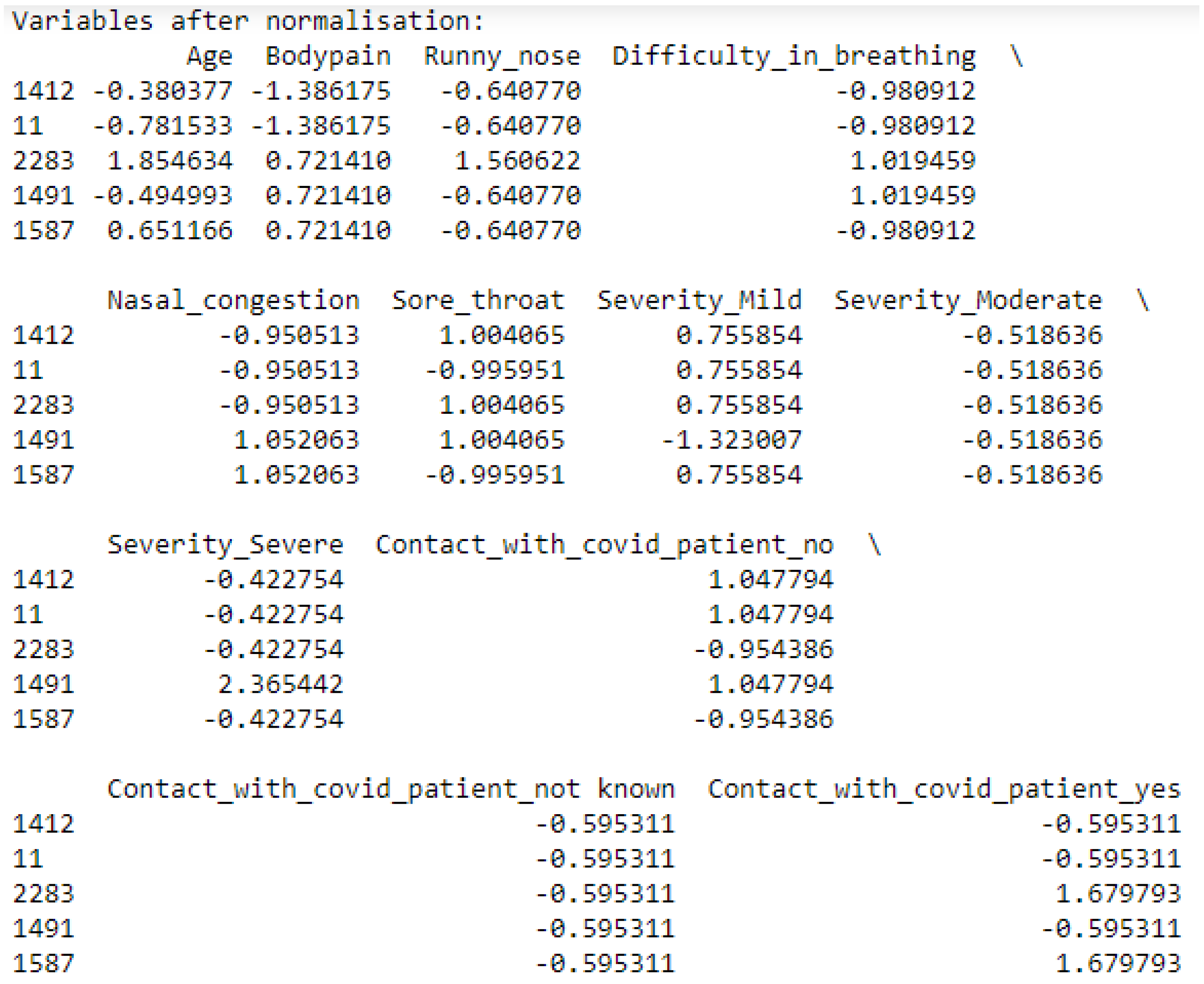
(2,3): In order to continue with the processing of our training and test data, we normalize the data, as shown in
Figure 9, by putting all quantitative variables on the same scale to avoid the size effect that skews the inertia (information) explained by the other variables with a reduced scale. This normalization is carried out according to the centered method reduced by standardscaler.
With X a quantitative variable, the mean of X and the standard deviation.
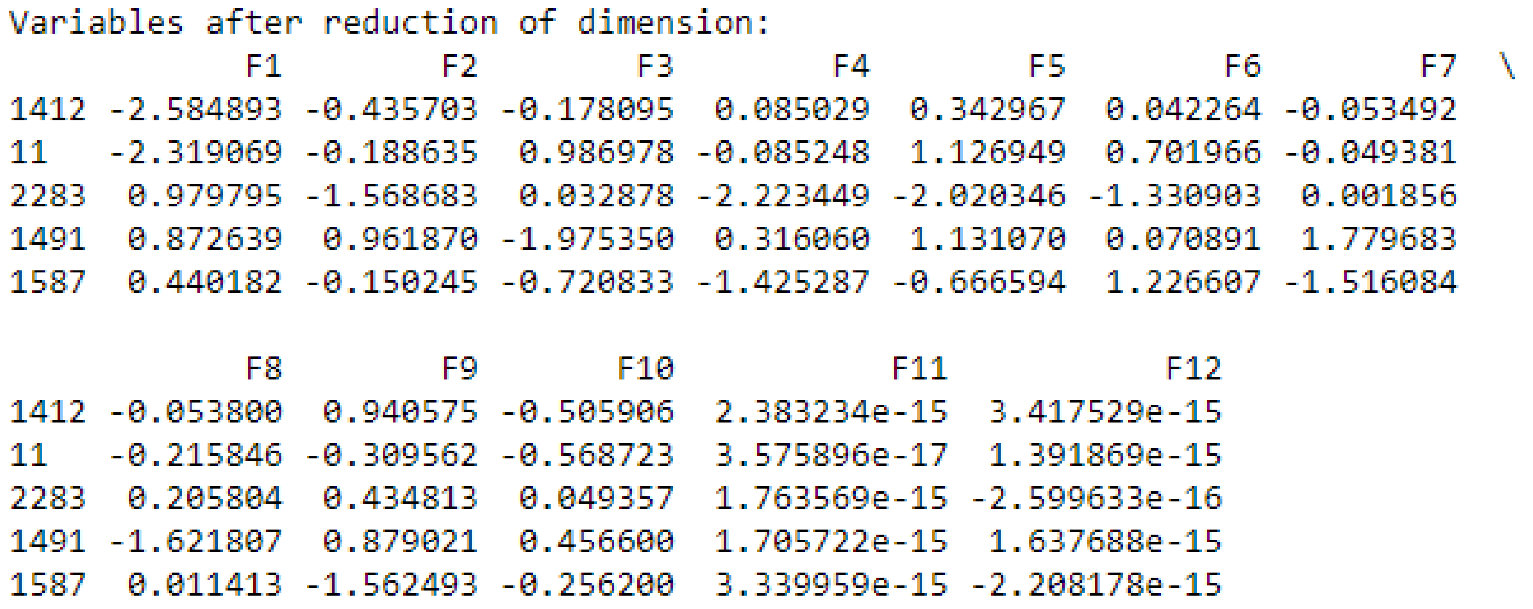
(4,5): After normalizing the data, we proceed to the dimension reduction by creating new components from the variables retained in step (1), as shown in
Figure 10. Each component is associated with a value to explain its contribution.
(6,7): Finally, we select the new variables that most synthesize all the starting information with the choice of the quantity to be retained fixed by threshold_ratio, as shown in
Figure 11.
The implementation of RF EP has yielded satisfactory results as presented in
Table 3.
5. Discussion
The objective of this study is to contribute to a decrease in the spread of COVID-19. To achieve this, we have undertaken to propose an enriched model of Random Forests, named Random Forests for Epidemiological Prediction (RF EP) with results that will allow us to achieve this goal. Our model implements the new Random Forests algorithm that we proposed and named Forest EP which is a modified version of Forest RI algorithm, the basic algorithm of default Random Forests.
In order to evaluate the effectiveness of RF EP, we based ourselves on the work of Buvana M. and MuthumayilK [
20] and then on an implementation of the default RF that we made ourselves. The results presented in
Table 2 in
Section 4, show that among the models evaluated by [
20], Decision Tree (DT) stands out as the best performer for all the metrics considered. On the same table we have inserted in the last row the results obtained with default Random Forests (RF) and we can observe, not surprisingly, that RF is better than DT for all metrics.
The results that are interesting to comment on here are those of RF EP presented in
Table 3 of
Section 4. The average of all default RF metrics is 0.95175 and that of RF EP is 0.95250, which is about an improvement of 0.001. Much more than this gross average of metrics, it is more interesting to analyze in detail the evolution of each metric.
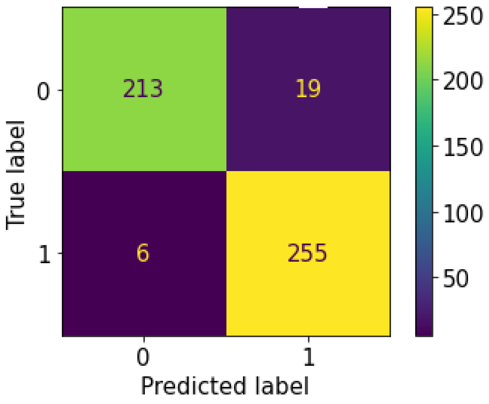
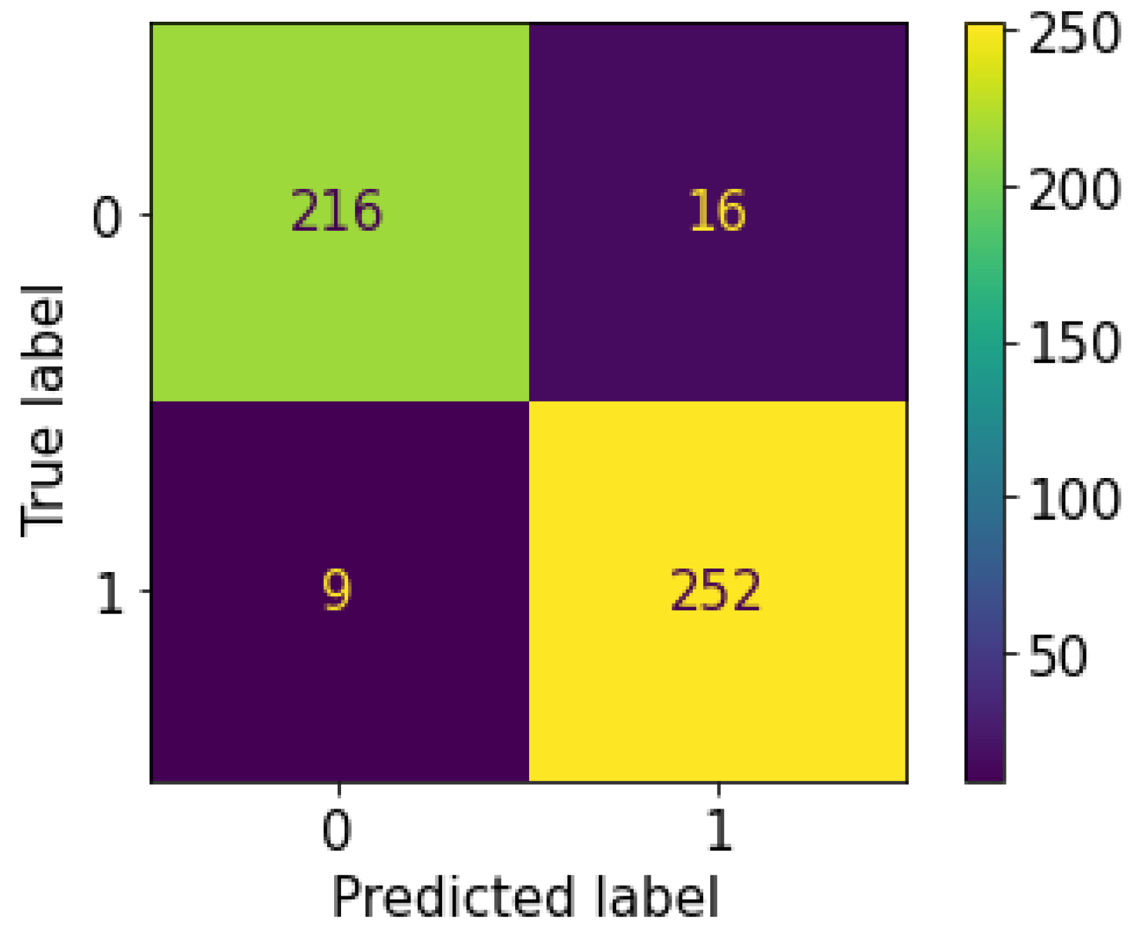
We notice that the values of the Accuracy metric are the same in both models (default RF and RF EP). This means that the total number of good predictions (positive and negative) is the same in both models. This can be verified on the default RF EP and RF confusion matrices presented in
Figure 12 and
Figure 13, respectively. For RF EP we have 213 TN + 255 TP = 468 and for default RF we have 216 TN + 252 TP = 468. The difference can therefore be made in the ability to correctly predict positive or negative cases. For this, it will be necessary to analyze the other metrics.
Regarding the Precision metric, RF EP records a performance loss of 0.009 compared to default RF. This means that the positive test provided by default RF is more reliable than the one provided by RF EP. Since positive tests are more reliable at default RF level, this means that negative tests are also reliable. Therefore, default RF will overall give fewer False Negative (FN) tests compared to RF EP. We can verify this on the confusion matrices of our implementation of both models on the test set: default RF has 16 FN while RF EP has 19 FN.
The result of Recall metric shows a performance gain of 0.011 for RF EP level compared to default RF. This means that RF EP has a better predictive ability regarding positive cases. In other words, when we consider the set of positive cases present in a dataset, with RF EP we will detect a greater number of cases compared to default RF. RF EP thus allows less missed detection of patients with COVID-19. However, because it is the positive patients who carry the disease and spread the virus, by increasing the model’s ability to detect them we have thus achieved the objective of this study. This can be verified on the confusion matrices of our implementation of the two models on the test dataset: default RF produced 252 TP and 9 FP while RF EP produced 255 TP and 6 FP. We see here that compared to patients who are actually positive default RF misclassified three people more than RF EP. This means that for our dataset three virus carriers are in the wild spreading the virus when they could have been detected using RF EP.
The F1 Score, which is the harmonic mean of the last two metrics, shows a performance gain of 0.001 of RF EP compared to the default RF.
6. Conclusions
The purpose of this paper was to propose a model to improve the fight against the spread of epidemics. The epidemic that has been chosen as an example is COVID-19. To do this, we used a dataset publicly accessible on GitHub that was designed for classification studies.
The predictive analysis performed was to determine whether a person is positive or negative for COVID-19 based on eleven variables, including: Country, Age, Fever, Bodypain, Runny_nose, Difficult_in_breathing, Nasal_congestion, Sore_throat, gender, Severity, and Contact_with_covid_patient. The target variable is named infected.
Most of the qualitative variables in this dataset were already encoded when we downloaded it except Gender, Severity, and Contact_with_covid_patient which we encoded ourselves using binary encoding for Gender and dummy encoding for Severity and Contact_with_covid_patient.
In this study, we propose an enriched model of Random Forests (RF). The choice of RF was based on a literature review of the research of several researchers who compared RF to other models in the context of epidemic predictions and placed RF at the top as the best classifier.
The enriched model of RF, named RF EP (EP for Epidemiological Prediction), implements an algorithm that we have proposed. This algorithm, named Forest EP, is a modified version of Forest RI, considered to be the main algorithm of RF which was proposed by Breiman L. Within Forest EP, we included the Var_Cust algorithm to perform four steps within RF itself without having to look for other methods outside. These four steps are: the selection of the significant variables, the normalization of the data, the dimension reduction in the dataset, and finally the selection of new variables that best synthesizes the information that the algorithm needs on the basis of the previously defined threshold_ratio.
Overall, our model performs satisfactorily. We first compared default RF with five other models: GNB, LR, SVM, KNN, and DT. Default RF stood out from all other models for all metrics considered; knowing that there were four: Accuracy, Precision, Recall, and F1 score. Compared to the default RF, RF EP has a performance improvement of 0.011 on the Recall metric. This improvement makes it possible to achieve the objective set at the outset of this study. This is because this performance gain means that RF EP is able to detect more positive patients than default RF for a given dataset. In other words, when a hospital or health center uses RF EP, they increase their ability to detect all positive patients, meaning that fewer people carrying the disease will be able to slip through the cracks of testing. We have with RF EP 255 TP and 6 FP while with default RF we have 252 TP and 9 FP on the same dataset.
Finally, we find it important to specify that this model, in order to be useful to health actors to contribute to the fight against epidemics, will be deployed in an environment that we have named MEPS (Mobile Epidemiological Prediction System). This is a mobile system that will use the model proposed in this paper and some tools from the ODK software suite to perform data collection and prediction in a hospital setting. This is a study that will be the subject of our next paper.
It should be noted that ODK is a very well known software suite used by health actors, mainly in developing countries. We have already worked on this software suite in the past, notably in [
45,
47,
48]. In our next work, we will propose an extension of ODK that will use the model proposed in this paper (RF EP).


