

Modeling and Compensation of Positioning Error in Micromanipulation
 ,
,
Abstract
:1. Introduction
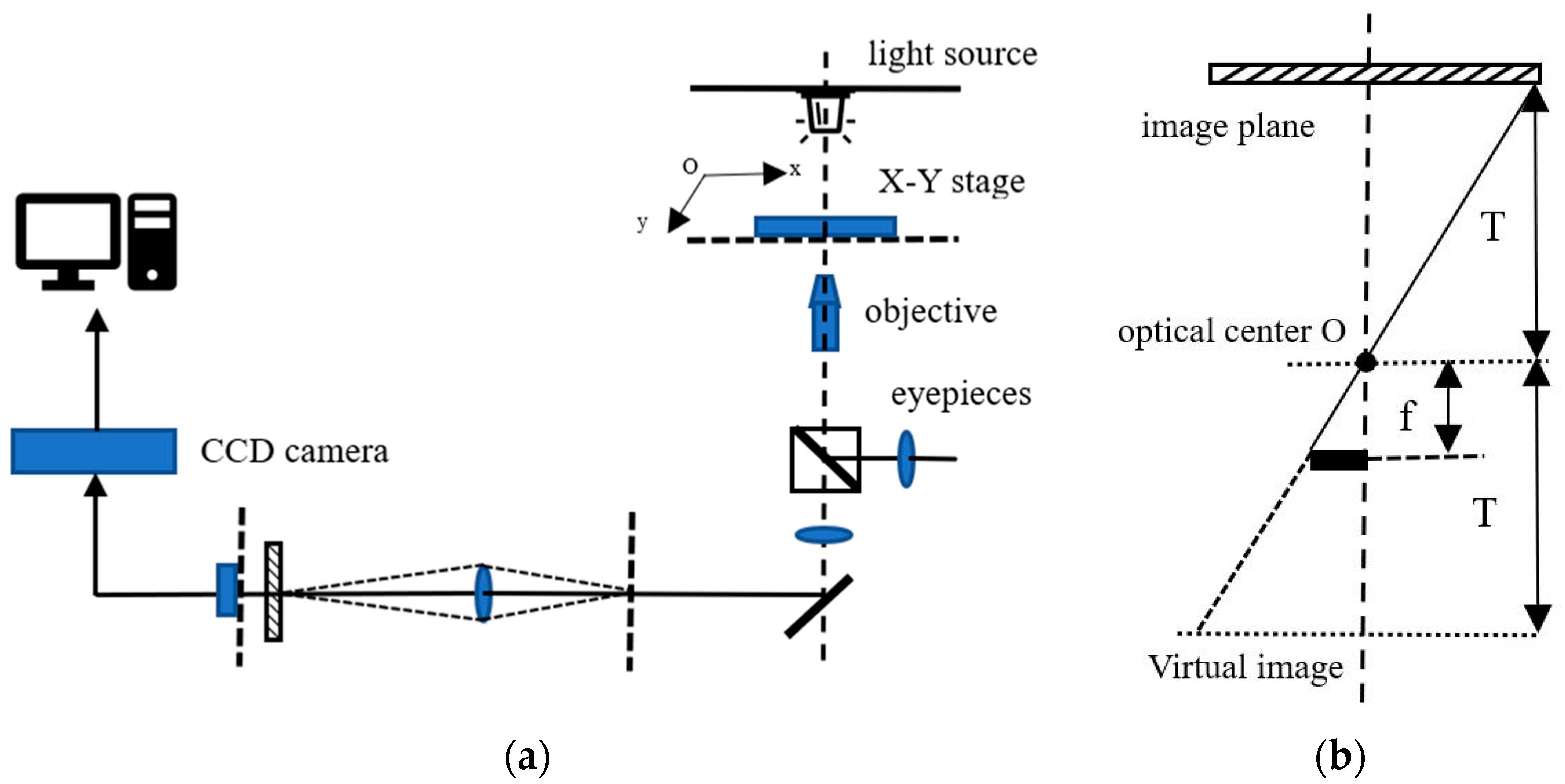
2. System Overview
3. Derivation of System Errors
3.1. Image Model Error
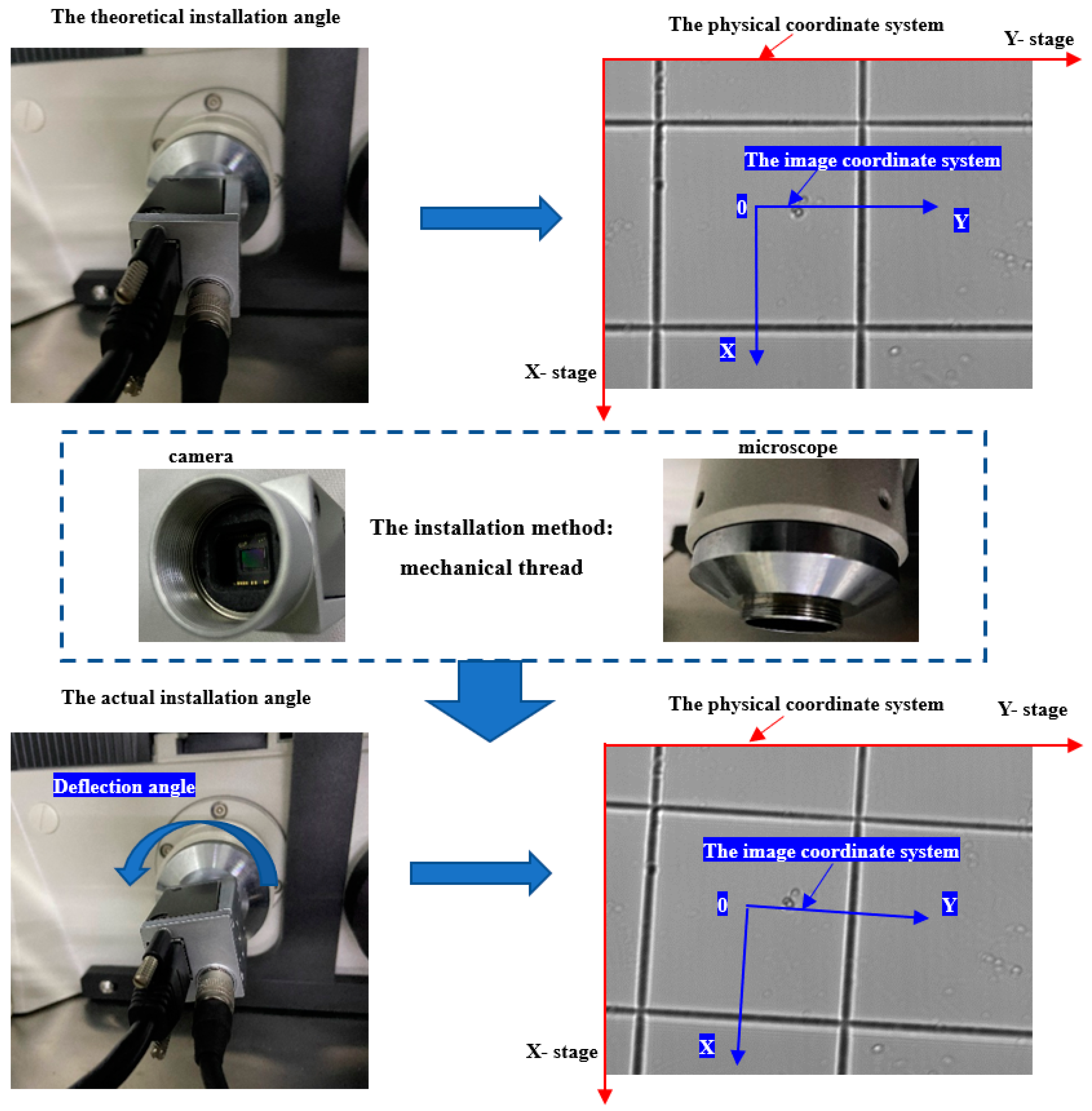
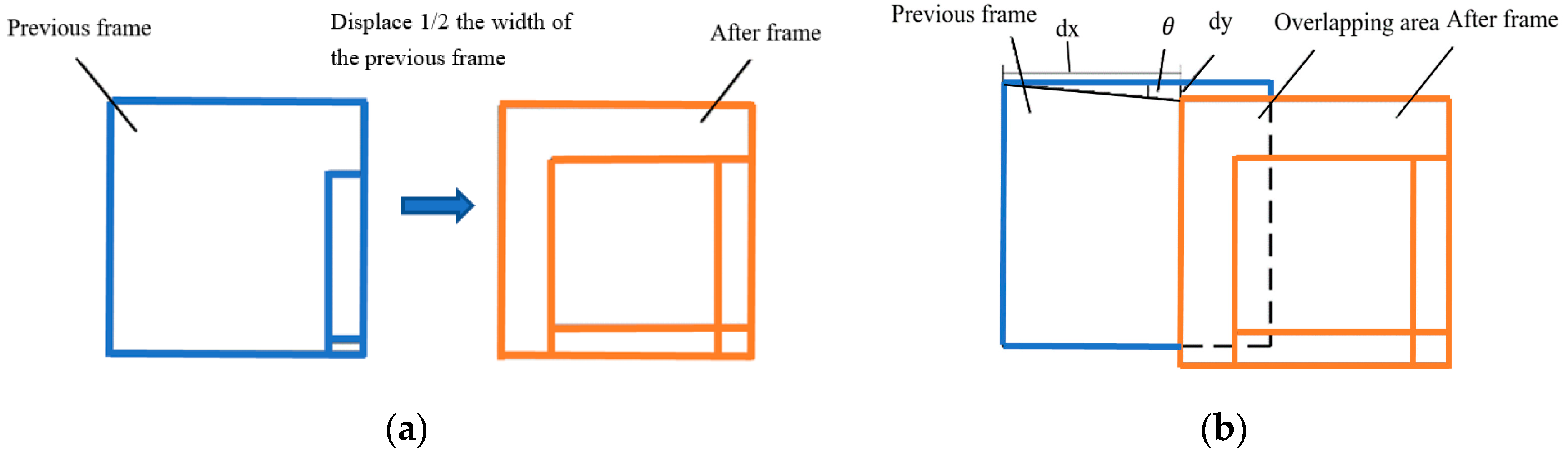
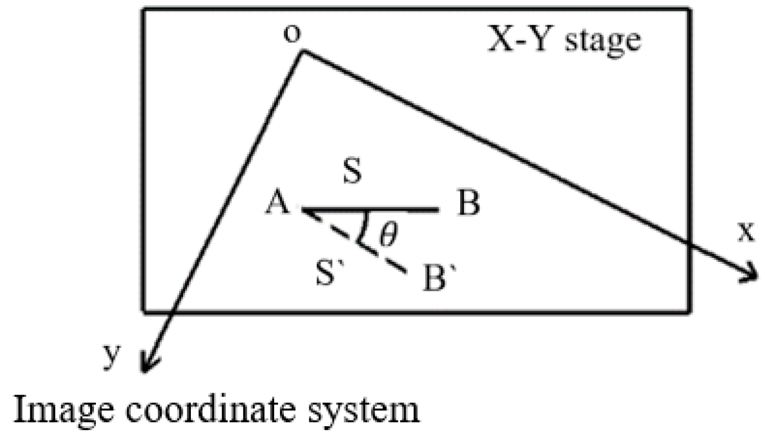
3.2. Camera Installation Error
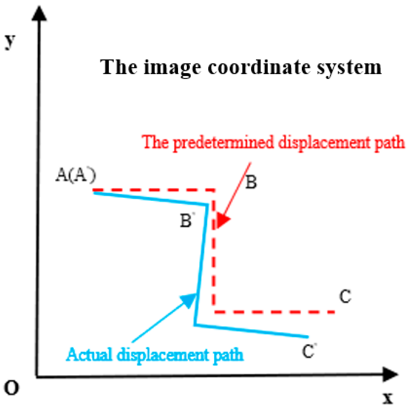
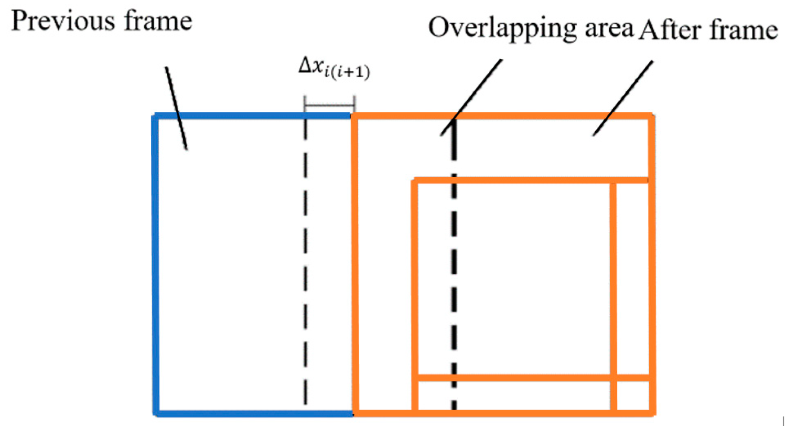
3.3. Mechanical Displacement Error
4. Establishment of Error Compensation Model
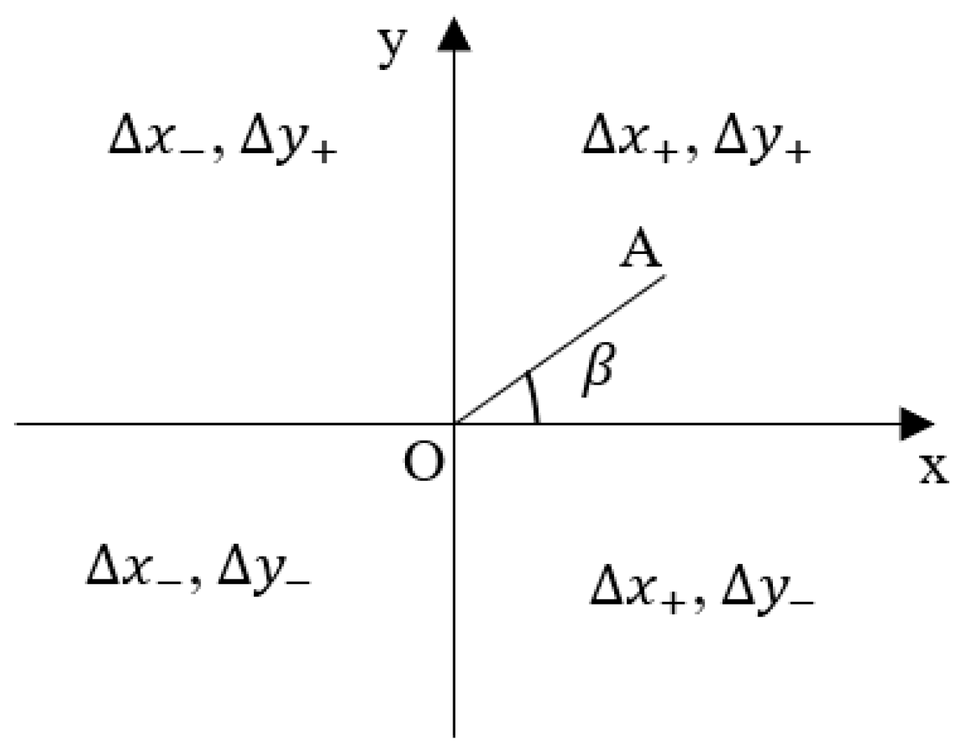
4.1. The Compensation Principles
4.2. Error Compensation Model
5. Experimental Results and Discussion
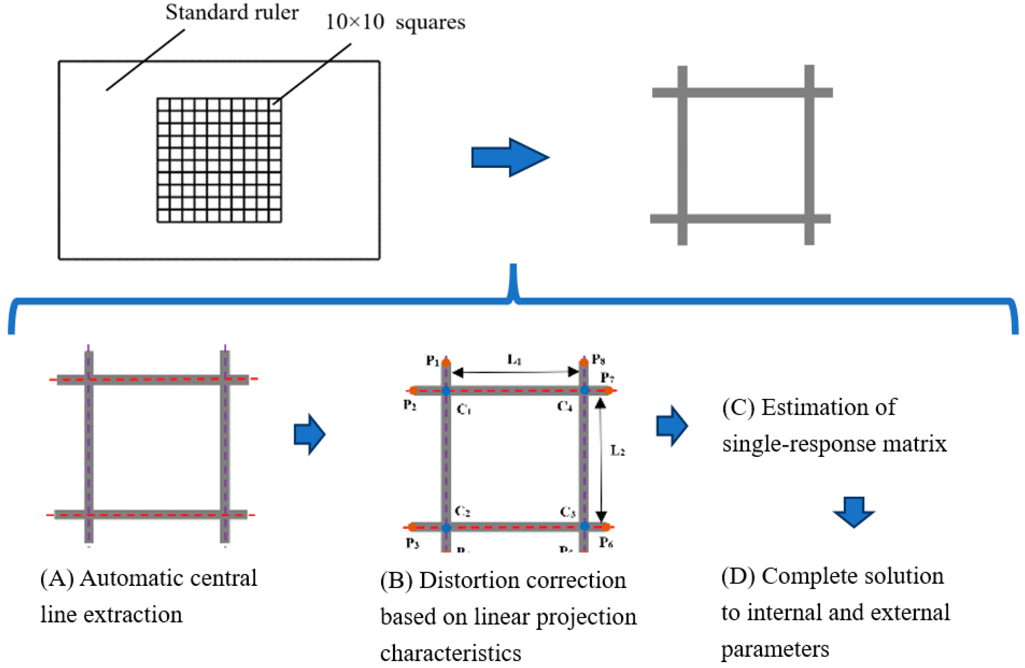
5.1. Calibration of Error Compensation Model
5.2. Single Shot Error Test
5.3. Cumulative Error Test
6. Conclusions
Author Contributions
Funding
Data Availability Statement
Conflicts of Interest
References
- Sariola, V.; Jääskeläinen, M.; Zhou, Q. Hybrid Microassembly Combining Robotics and Water Droplet Self-Alignment. IEEE Trans. Robot. 2010, 26, 965–977. [Google Scholar] [CrossRef]
- Rodríguez, J.A.M. Microscope self-calibration based on micro laser line imaging and soft computing algorithms. Opt. Lasers Eng. 2018, 105, 75–85. [Google Scholar] [CrossRef]
- Gorpas, D.S.; Politopoulos, K.; Yova, D. Development of a computer vision binocular system for non-contact small animal model skin cancer tumour imaging. In Proceedings of the SPIE Diffuse Optical Imaging of Tissue, Munich, Germany, 12–17 June 2007; pp. 6629–6656. [Google Scholar]
- Su, L.; Zhang, H.; Wei, H.; Zhang, Z.; Yu, Y.; Si, G.; Zhang, X. Macro-to-micro positioning and auto focusing for fully automated single cell microinjection. Microsyst. Technol. 2021, 27, 11–21. [Google Scholar] [CrossRef]
- Wang, Y.Z.; Geng, B.L.; Long, C. Contour extraction of a laser stripe located on a microscope image from a stereo light microscope. Microsc. Res. Tech. 2019, 82, 260–271. [Google Scholar] [CrossRef]
- Wu, H.; Zhang, X.M.; Gan, J.Q.; Li, H.; Ge, P. Displacement measurement system for inverters using computer micro-vision. Opt. Lasers Eng. 2016, 81, 113–118. [Google Scholar] [CrossRef] [Green Version]
- Sha, X.P.; Li, W.C.; Lv, X.Y.; Lv, J.T.; Li, Z.Q. Research on auto-focusing technology for micro vision system. Optik 2017, 142, 226–233. [Google Scholar] [CrossRef]
- Tsai, R. A versatile camera calibration technique for high-accuracy 3D machine vision metrology using off-the-shelf TV cameras and lenses. IEEE J. Robot Autom. 1987, 3, 323–344. [Google Scholar] [CrossRef] [Green Version]
- Korpelainen, V.; Seppä, J.; Lassila, A. Design and characterization of MIKES metrological atomic force microscope. Precis. Eng. 2010, 34, 735–744. [Google Scholar] [CrossRef]
- Steger, C. A comprehensive and Versatile Camera Model for Cameras with Tilt Lenses. Int. J. Comput. Vis. 2017, 123, 121–159. [Google Scholar] [CrossRef] [Green Version]
- Lee, K.H.; Kim, H.S.; Lee, S.J.; Choo, S.W.; Lee, S.M.; Nam, K.T. High precision hand-eye self-calibration for industrial robots. In Proceedings of the 2018 International Conference on Electronics, Information, and Communication (ICEIC), Honolulu, HI, USA, 24–27 January 2018. [Google Scholar]
- Maraghechi, S.; Hoefnagels, J.P.; Peerlings, R.H.; Rokoš, O.; Geers, M.G. Correction of scanning electron microscope imaging artifacts in a novel digital image correlation framework. Exp. Mech. 2019, 59, 489–516. [Google Scholar] [CrossRef] [Green Version]
- Lapshin, R. Drift-insensitive distributed calibration of probe microscope scanner in nanometer range: Real mode. Appl. Surf. Sci. 2019, 470, 1122–1129. [Google Scholar] [CrossRef] [Green Version]
- Yothers, M.; Browder, A.; Bumm, A. Real-space post-processing correction of thermal drift and piezoelectric actuator nonlinearities in scanning tunneling microscope images. Rev. Sci. Instrum. 2017, 88, 013708. [Google Scholar] [CrossRef] [Green Version]
- Liu, X.; Li, Z.; Zhong, K.; Chao, Y.; Miraldo, P.; Shi, Y. Generic distortion model for metrology under optical microscopes. Opt. Laser Eng. 2018, 103, 119–126. [Google Scholar] [CrossRef]
- Yoneyama, S.; Kitagawa, A.; Kitamura, K.; Kikuta, H. In-plane displacement measurement using digital image correlation with lens distortion correction. JSME Int. 2006, 49, 458–467. [Google Scholar] [CrossRef] [Green Version]
- Yoneyama, S.; Kikuta, H.; Kitagawa, A.; Kitamura, K. Lens distortion correction for digital image correlation by measuring rigid body displacement. Opt. Eng. 2006, 45, 023602. [Google Scholar] [CrossRef]
- Pan, B.; Yu, L.; Wu, D.; Tang, L. Systematic errors in two-dimensional digital image correlation due to lens distortion. Opt. Laser Eng. 2013, 51, 140–147. [Google Scholar] [CrossRef]
- Tiwari, V.; Sutton, M.A.; McNeill, S.R. Assessment of high speed imaging systems for 2D and 3D deformation measurements: Methodology development and validation. Exp. Mech. 2007, 47, 561–579. [Google Scholar] [CrossRef]
- Koide, K.; Menegatti, E. General hand-eye calibration based on reprojection error minimization. IEEE Robot. Autom. Lett. 2019, 4, 1021–1028. [Google Scholar] [CrossRef]
- Malti, A. Hand–eye calibration with epipolar constraints: Application to endoscopy. Robot. Auton. Syst. 2013, 61, 161–169. [Google Scholar] [CrossRef]
- Hartley, R.; Kang, S.B. Parameter-free radial distortion correction with center of distortion estimation. IEEE Trans. Pattern Anal. Mach. Intell. 2007, 29, 1309–1321. [Google Scholar] [CrossRef] [Green Version]
- Lowe, D.G. Distinctive image features from scale-invariant keypoints. Int. J. Comput. Vis. 2004, 60, 91–110. [Google Scholar] [CrossRef]
- Fischler, M.A.; Bolles, R.C. Random sample consensus: A paradigm for model fitting with applications to image analysis and automated cartography. Commun. ACM 1981, 24, 381–395. [Google Scholar] [CrossRef]


| Parameters | Theoretical Values | Actual Values |
|---|---|---|
(pixel/µm) | 1 | 0.993 |
(pixel/µm) | 1 | 0.992 |
(pixel) | (600.0,450.0) | (600.3,450.2) |
(pixel)−2 | 0 | 0.0122 |
| 20 | 19.843 | |
| 1 | 0.9922 | |
| 0 | −2.3718 | |
| 0 | −2.7474 |
| Groups | Result of Error Compensation Coefficient θ | ||
|---|---|---|---|
| dy (pix) | dx (pix) | ||
| 1 | −30 | 304 | −5.636 |
| 2 | −29 | 306 | −5.414 |
| 3 | −30 | 308 | −5.563 |
| 4 | −31 | 308 | −5.747 |
| 5 | −29 | 303 | −5.467 |
| 6 | −30 | 307 | −5.581 |
| 7 | −30 | 306 | −5.599 |
| 8 | −31 | 308 | −5.747 |
| 9 | −29 | 305 | −5.431 |
| 10 | −30 | 306 | −5.599 |
| average | - | - | −5.578 |
| Groups | (pix) | (pix) | (pix) | (pix) |
|---|---|---|---|---|
| 1 | −3 | −4 | −6 | −4 |
| 2 | −7 | −6 | −6 | −5 |
| 3 | −6 | −8 | −6 | −5 |
| 4 | −5 | −8 | −5 | −7 |
| 5 | −5 | −6 | −5 | −6 |
| 6 | −4 | −5 | −7 | −5 |
| 7 | −3 | −7 | −5 | −4 |
| 8 | −6 | −5 | −6 | −5 |
| 9 | −7 | −4 | −5 | −6 |
| 10 | −6 | −5 | −6 | −5 |
| average | −5.2 | −5.8 | −5.7 | −5.2 |
| Classification | Groups | The Step Length (μm) | Total Number of Images in a Group | Number of Displacement Images in One Direction | Total Step Length in One Direction (μm) |
|---|---|---|---|---|---|
| 1 | 1–10 | 600 | 5 | 2 | 1800 |
| 2 | 11–20 | 600 | 9 | 3 | 2400 |
| 3 | 21–30 | 600 | 13 | 4 | 3000 |
| 4 | 31–40 | 600 | 17 | 5 | 3600 |
| 5 | 41–50 | 600 | 21 | 6 | 4200 |
Disclaimer/Publisher’s Note: The statements, opinions and data contained in all publications are solely those of the individual author(s) and contributor(s) and not of MDPI and/or the editor(s). MDPI and/or the editor(s) disclaim responsibility for any injury to people or property resulting from any ideas, methods, instructions or products referred to in the content. |
© 2023 by the authors. Licensee MDPI, Basel, Switzerland. This article is an open access article distributed under the terms and conditions of the Creative Commons Attribution (CC BY) license (https://creativecommons.org/licenses/by/4.0/).
Share and Cite
Hao, M.; Yang, B.; Ru, C.; Yue, C.; Huang, Z.; Zhai, R.; Sun, Y.; Wang, Y.; Dai, C. Modeling and Compensation of Positioning Error in Micromanipulation. Micromachines 2023, 14, 779. https://doi.org/10.3390/mi14040779
Hao M, Yang B, Ru C, Yue C, Huang Z, Zhai R, Sun Y, Wang Y, Dai C. Modeling and Compensation of Positioning Error in Micromanipulation. Micromachines. 2023; 14(4):779. https://doi.org/10.3390/mi14040779
Chicago/Turabian StyleHao, Miao, Bin Yang, Changhai Ru, Chunfeng Yue, Zongjie Huang, Rongan Zhai, Yu Sun, Yong Wang, and Changsheng Dai. 2023. "Modeling and Compensation of Positioning Error in Micromanipulation" Micromachines 14, no. 4: 779. https://doi.org/10.3390/mi14040779