
Theoretical Analysis and Experimental Verification of the Influence of Polarization on Counter-Propagating Optical Tweezers
 , and
, and 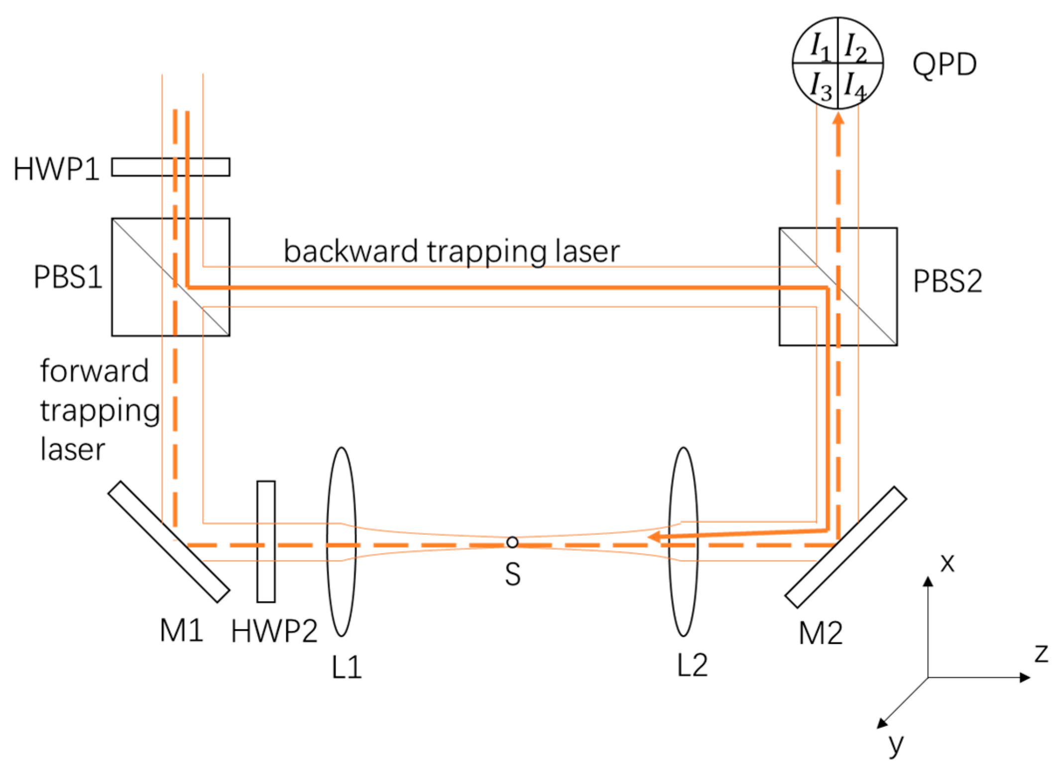
Abstract
:1. Introduction
2. Materials and Methods
2.1. T-Matrix Method
2.2. Experimental Setup
3. Results
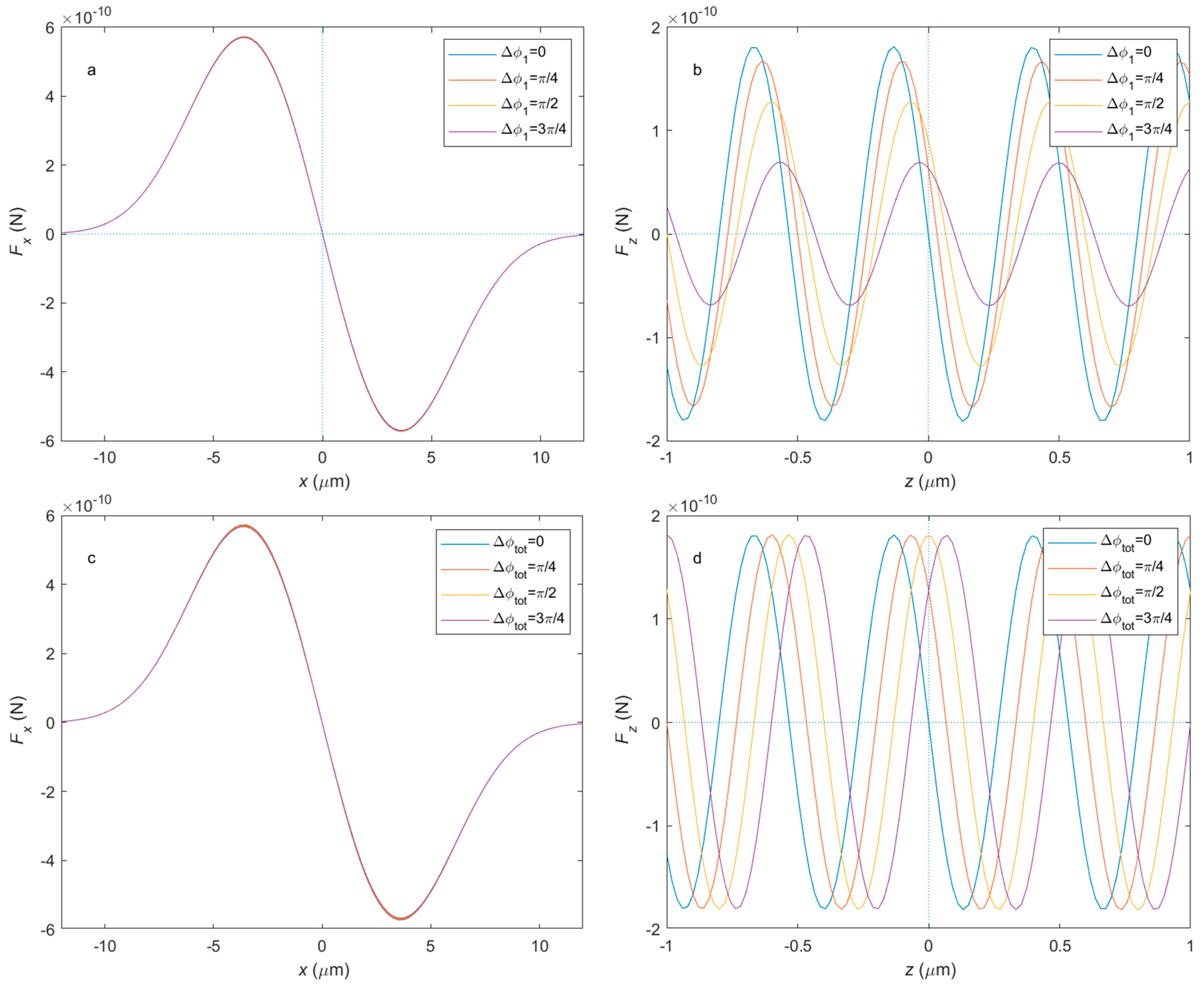
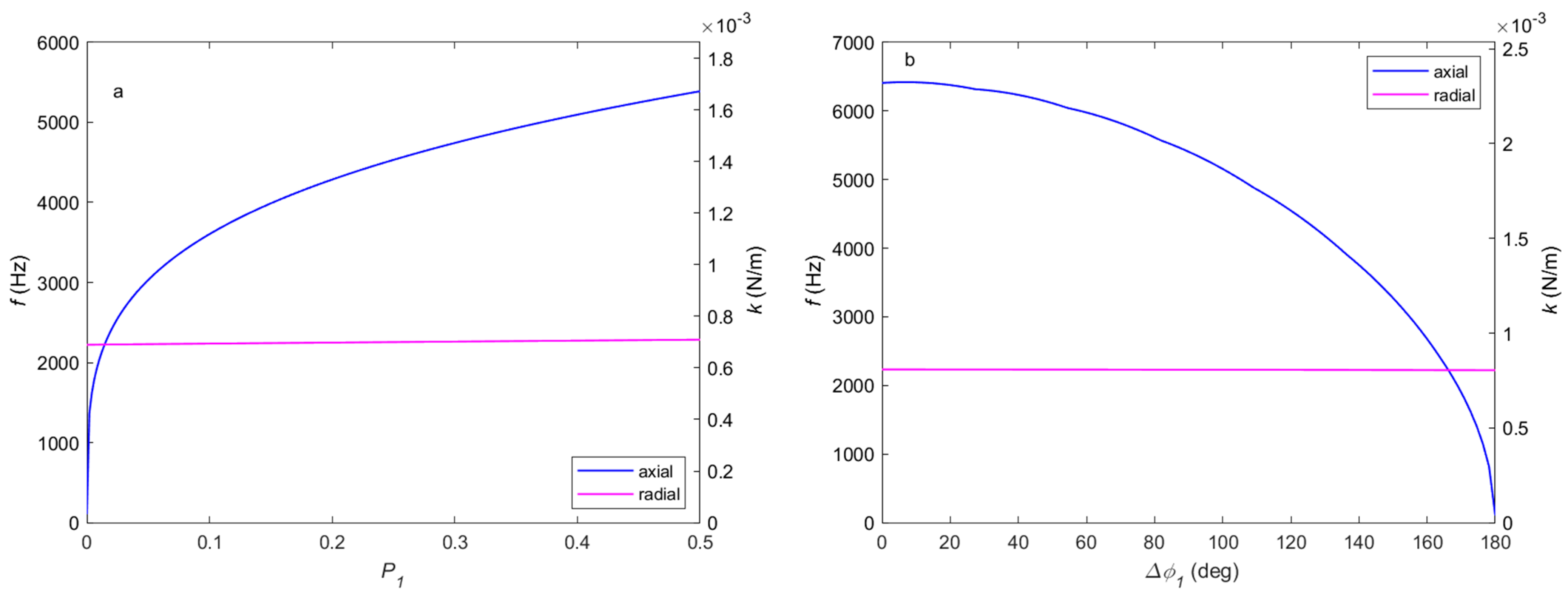
3.1. Numerical Analysis
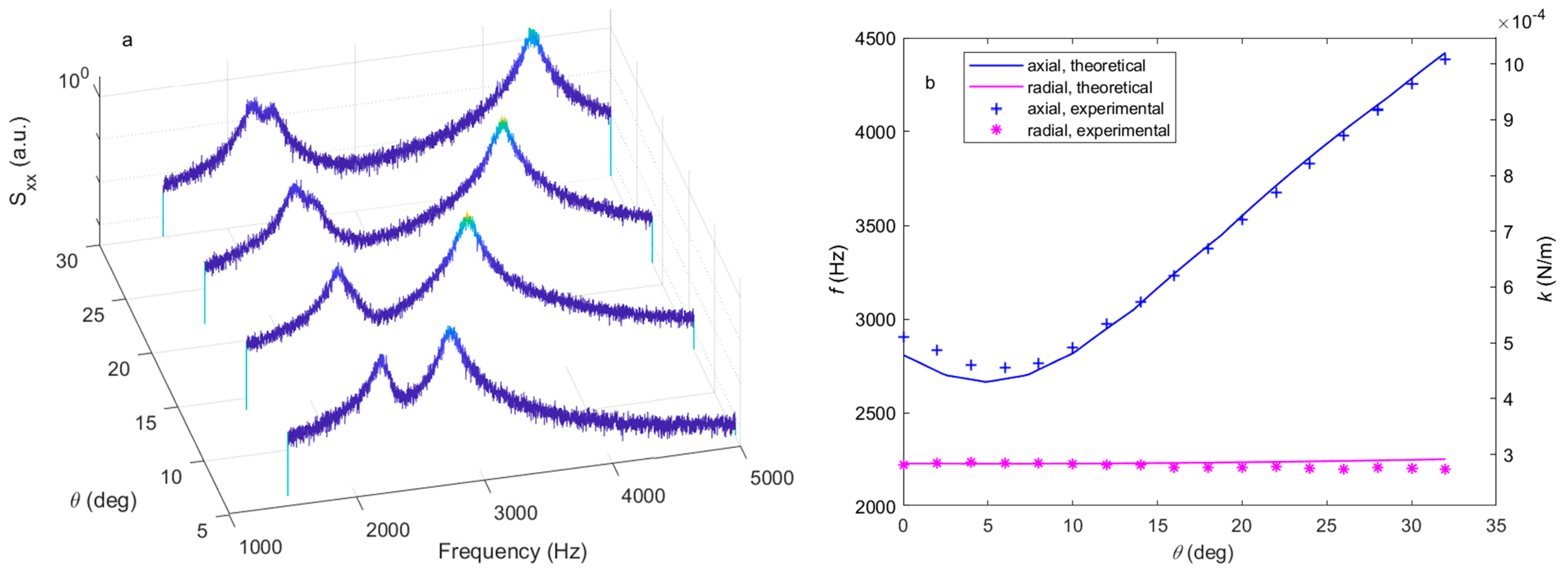
3.2. Experimental Verification
4. Discussion
Author Contributions
Funding
Data Availability Statement
Conflicts of Interest
References
- Ashkin, A. Acceleration and Trapping of Particles by Radiation Pressure. Phys. Rev. Lett. 1970, 24, 156–159. [Google Scholar] [CrossRef] [Green Version]
- Shabestari, M.H.; Meijering, A.E.C.; Roos, W.H.; Wuite, G.J.L.; Peterman, E.J.G. Recent advances in biological single-molecule applications of optical tweezers and fluorescence microscopy. Methods Enzymol. 2017, 582, 85–119. [Google Scholar]
- Grier, D.G. Optical tweezers in colloid and interface science. Curr. Opin. Colloid Interface Sci. 1997, 2, 264–270. [Google Scholar] [CrossRef]
- Kaufman, A.M.; Lester, B.J.; Reynolds, C.M.; Wall, M.L.; Foss-Feig, M.; Hazzard, K.R.A.; Rey, A.M.; Regal, C.A. Two-particle quantum interference in tunnel-coupled optical tweezers. Science 2014, 345, 306–309. [Google Scholar] [CrossRef] [PubMed] [Green Version]
- Geraci, A.A.; Papp, S.B.; Kitching, J. Short-range force detection using optically cooled levitated microspheres. Phys. Rev. Lett. 2010, 105, 101101. [Google Scholar] [CrossRef] [PubMed] [Green Version]
- Ranjit, G.; Cunningham, M.; Casey, K.; Geraci, A.A. Zeptonewton force sensing with nanospheres in an optical lattice. Phys. Rev. A 2016, 93, 053801. [Google Scholar] [CrossRef] [Green Version]
- Gieseler, J.; Gomez-Solano, J.R.; Magazzù, A.; Castillo, I.P.; García, L.P.; Gironella-Torrent, M.; Viader-Godoy, X.; Ritort, F.; Pesce, G.; Arzola, A.V.; et al. Optical tweezers—From calibration to applications: A tutorial. Adv. Opt. Photonics 2021, 13, 74–241. [Google Scholar] [CrossRef]
- Ashkin, A. Forces of a single-beam gradient laser trap on a dielectric sphere in the ray optics regime. Biophys. J. 1992, 61, 569–582. [Google Scholar] [CrossRef] [PubMed] [Green Version]
- Tebbenjohanns, F.; Frimmer, M.; Novotny, L. Optimal position detection of a dipolar scatterer in a focused field. Phys. Rev. A 2019, 100, 043821. [Google Scholar] [CrossRef] [Green Version]
- Hu, M.; Li, N.; Li, W.; Wang, X.; Hu, H. Fdtd simulation of optical force under non-ideal conditions. Opt. Commun. 2022, 505, 127586. [Google Scholar] [CrossRef]
- Nieminen, T.A.; Loke, V.L.; Stilgoe, A.B.; Knöner, G.; Brańczyk, A.M.; Heckenberg, N.R.; Rubinsztein-Dunlop, H. Optical tweezers computational toolbox. J. Opt. A Pure Appl. Opt. 2007, 9, S196. [Google Scholar] [CrossRef] [Green Version]
- van der Horst, A.; Campbell, A.I.; van Vugt, L.K.; Vanmaekelbergh, D.A.; Dogterom, M.; van Blaaderen, A. Manipulating metal-oxide nanowires using counter-propagating optical line tweezers. Opt. Express 2007, 15, 11629–11639. [Google Scholar] [CrossRef] [PubMed]
- Zhang, Y.; Dai, Y. Multifocal optical trapping using counter-propagating radially-polarized beams. Opt. Commun. 2012, 285, 725–730. [Google Scholar] [CrossRef]
- Jones, R.C. A new calculus for the treatment of optical systemsi. description and discussion of the calculus. Josa 1941, 31, 488–493. [Google Scholar] [CrossRef]
- Taylor, M.A.; Bowen, W.P. A computational tool to characterize particle trackingmeasurements in optical tweezers. J. Opt. 2013, 15, 5701. [Google Scholar] [CrossRef]
- Li, T.; Li, T. Millikelvin cooling of an optically trapped microsphere in vacuum. Fundam. Tests Phys. Opt. Trapped Microspheres 2013, 81–110. [Google Scholar]
- Berg-Sørensen, K.; Flyvbjerg, H. Power spectrum analysis for optical tweezers. Rev. Sci. Instrum. 2004, 75, 594–612. [Google Scholar] [CrossRef] [Green Version]
- Gieseler, J.; Deutsch, B.; Quidant, R.; Novotny, L. Subkelvin parametric feedback cooling of of a laser-trapped nanoparticle. Phys. Rev. Lett. 2012, 109, 103603. [Google Scholar] [CrossRef] [PubMed] [Green Version]


Disclaimer/Publisher’s Note: The statements, opinions and data contained in all publications are solely those of the individual author(s) and contributor(s) and not of MDPI and/or the editor(s). MDPI and/or the editor(s) disclaim responsibility for any injury to people or property resulting from any ideas, methods, instructions or products referred to in the content. |
© 2023 by the authors. Licensee MDPI, Basel, Switzerland. This article is an open access article distributed under the terms and conditions of the Creative Commons Attribution (CC BY) license (https://creativecommons.org/licenses/by/4.0/).
Share and Cite
Chen, M.; Li, W.; Yang, J.; Hu, M.; Xu, S.; Zhu, X.; Li, N.; Hu, H. Theoretical Analysis and Experimental Verification of the Influence of Polarization on Counter-Propagating Optical Tweezers. Micromachines 2023, 14, 760. https://doi.org/10.3390/mi14040760
Chen M, Li W, Yang J, Hu M, Xu S, Zhu X, Li N, Hu H. Theoretical Analysis and Experimental Verification of the Influence of Polarization on Counter-Propagating Optical Tweezers. Micromachines. 2023; 14(4):760. https://doi.org/10.3390/mi14040760
Chicago/Turabian StyleChen, Ming, Wenqiang Li, Jianyu Yang, Mengzhu Hu, Shidong Xu, Xunmin Zhu, Nan Li, and Huizhu Hu. 2023. "Theoretical Analysis and Experimental Verification of the Influence of Polarization on Counter-Propagating Optical Tweezers" Micromachines 14, no. 4: 760. https://doi.org/10.3390/mi14040760