Global Data Sets of Vegetation Leaf Area Index (LAI)3g and Fraction of Photosynthetically Active Radiation (FPAR)3g Derived from Global Inventory Modeling and Mapping Studies (GIMMS) Normalized Difference Vegetation Index (NDVI3g) for the Period 1981 to 2011

 , ,
, ,
Abstract
: Long-term global data sets of vegetation Leaf Area Index (LAI) and Fraction of Photosynthetically Active Radiation absorbed by vegetation (FPAR) are critical to monitoring global vegetation dynamics and for modeling exchanges of energy, mass and momentum between the land surface and planetary boundary layer. LAI and FPAR are also state variables in hydrological, ecological, biogeochemical and crop-yield models. The generation, evaluation and an example case study documenting the utility of 30-year long data sets of LAI and FPAR are described in this article. A neural network algorithm was first developed between the new improved third generation Global Inventory Modeling and Mapping Studies (GIMMS) Normalized Difference Vegetation Index (NDVI3g) and best-quality Terra Moderate Resolution Imaging Spectroradiometer (MODIS) LAI and FPAR products for the overlapping period 2000–2009. The trained neural network algorithm was then used to generate corresponding LAI3g and FPAR3g data sets with the following attributes: 15-day temporal frequency, 1/12 degree spatial resolution and temporal span of July 1981 to December 2011. The quality of these data sets for scientific research in other disciplines was assessed through (a) comparisons with field measurements scaled to the spatial resolution of the data products, (b) comparisons with broadly-used existing alternate satellite data-based products, (c) comparisons to plant growth limiting climatic variables in the northern latitudes and tropical regions, and (d) correlations of dominant modes of interannual variability with large-scale circulation anomalies such as the EI Niño-Southern Oscillation and Arctic Oscillation. These assessment efforts yielded results that attested to the suitability of these data sets for research use in other disciplines. The utility of these data sets is documented by comparing the seasonal profiles of LAI3g with profiles from 18 state-of-the-art Earth System Models: the models consistently overestimated the satellite-based estimates of leaf area and simulated delayed peak seasonal values in the northern latitudes, a result that is consistent with previous evaluations of similar models with ground-based data. The LAI3g and FPAR3g data sets can be obtained freely from the NASA Earth Exchange (NEX) website.1. Introduction
Monitoring and modeling global vegetation dynamics in the context of climate variability and change studies require long-term data sets of key biophysical variables that characterize vegetation structure and functioning [1]. Leaf Area Index (LAI) and the Fraction of Photosynthetically Active Radiation absorbed by vegetation (FPAR) are two examples of such variables. LAI is defined as the one-sided green leaf area per unit vegetated ground area in broadleaf canopies and as one-half the total needle surface area per unit vegetated ground area in coniferous canopies. It characterizes the physiologically functioning surface area with which energy, mass (e.g., water and CO2) and momentum are exchanged between the vegetated land surface and the planetary boundary layer [2]. Similarly, FPAR is a relative measure of the vegetation-absorbed radiation in the 0.4–0.7 μm spectral region of solar radiation, and hence, characterizes the energy that is potentially used in the process of photosynthesis. LAI and FPAR are therefore key state variables in many biogeochemical, ecological, hydrological and crop yield models [3–17].
There are several different approaches for estimating LAI and FPAR from remotely sensed reflectance data in the optical domain, i.e., the wavelength span of solar radiation. They can be broadly be categorized as:
Empirical methods based on relationships between vegetation indices, e.g., the Normalized Difference Vegetation Index (NDVI), and LAI or FPAR [18,19]. These relationships are generally sensitive to soil background, leaf optical properties, the orientation and spatial distribution of leaves in a canopy and the general architecture of vegetation stands within the spatial scale of measurements [20]. Site- and vegetation-specific empirical relationships between NDVI and LAI, for example, have been used in some studies [21,22]. The relationships tend to vary seasonally and inter-annually. Consequently, empirical methods tend to be site-, time-, and species-specific, and are therefore not well-suited for large-scale operational use [23].
Physical methods based on the physics of radiation interaction with elements of a canopy and transport within the vegetative medium. These methods provide a physically-based linkage between biophysical variables and vegetation canopy reflectance at different wavelengths [24–26]. These methods can be categorized into four broad groups: (1) radiative transfer models [24,25], (2) geometric-optical models [27], (3) hybrid models that incorporate both radiative transfer as well as geometric-optics [28], and (4) Monte-Carlo simulation models [29,30]. The methods involve iterative techniques and are thus computationally intensive for operational use. But, methods to alleviate this have also been developed, e.g., use of Look-Up-Tables [25].
Machine learning algorithms that are accurate, fast and require less computational power are increasingly being used lately to mimic the underlying physical processes in the remote sensing of vegetation [31–33]. The efficacy of these algorithms is dependent on a knowledge-based inference paradigm that is dependent on the robustness and availability of training data.
LAI and FPAR products from the Moderate Resolution Imaging Spectroradiometer (MODIS) and the Système Pour l’Observation de la Terre (SPOT) sensor have gradually acquired a large user community due to ease of access, provision of pixel-level quality indicators and validation information. Research on inter-sensor product consistency and collaborative validation efforts have helped provide accuracy and precision information of existing products [34–40]. A decade-long global and regional data sets of LAI and FPAR from these sensors are now available for scientific use. These records will likely be extended by the Visible/Infrared Imager Radiometer Suite instrument onboard the Suomi National Polar-orbiting Partnership, the Advanced Baseline Imager onboard the Geostationary Operational Environmental Satellite-R series satellite, the Charge-Coupled Device onboard the Huan Jing series satellites and the Advanced Visible and Near Infrared Radiometer onboard Advanced Land Observation Satellite [41–45]. These existing products are of short time span, thus precluding determination of long-term trends. Thus, there is a continuing interest and need for utilizing data from the Advanced Very High Resolution Radiometers (AVHRR) sensors, which is now more than three decades long and continuing.
The first generation NDVI data (NDVIg) from AVHRR sensors onboard the National Oceanic and Atmospheric Administration (NOAA) 7 to 14 series of satellites have been processed by the Global Inventory Modeling and Mapping Studies (GIMMS) group to a consistent time series of NDVI and is made available to the research community [46]. The latest version, termed the third generation NDVI data set (GIMMS NDVI3g) has been recently produced for the period July 1981 to December 2011 with AVHRR sensor data from NOAA 7 to 18 satellites. This data set specifically aims to improved data quality in the high latitudes where the growing season is shorter than 2 months. It has also improved calibration that is tied to the Sea-Viewing Wide-Field-of-View Sensor, as opposed to earlier versions of GIMMS NDVI data sets that were based on inter-calibration with the SPOT sensor. The availability of this new improved NDVI3g data set and its overlap with the Terra MODIS LAI and FPAR products for the period 2000 to 2009 provides an opportunity to design and implement a neural network algorithm to generate and evaluate the corresponding LAI and FPAR data sets—that is the objective of this article. These data sets will be termed LAI3g and FPAR3g henceforth and have the following attributes: 15-day temporal frequency, 1/12 degree spatial resolution and temporal span of July 1981 to December 2011.
This following presentation is organized as follows. Section 2 describes the algorithmic details and generation of the LAI3g and FPAR3g data sets. Section 3 is focused on validation and evaluation of these data sets in order to assess their suitability for research use in other disciplines. Section 4 describes a test case where the seasonal profiles of LAI3g are compared to simulations from 18 state-of-the-art Earth System Models to document the utility of these data sets. Concluding remarks are briefly stated in Section 5.
2. Production of LAI3g and FPAR3g Data Sets
2.1. Input Data and Preprocessing
We used improved versions of Collection 5 Terra MODIS LAI and FPAR products and the NDVI3g data for developing the algorithm. The MODIS BNU (Beijing Normal University version) LAI product is an improved version of the standard MODIS LAI product (MOD15A2) which provides 8 day global LAI data from 2000 to 2009 at 1 km spatial resolution [47]. The MODIS BU (Boston University) FPAR product is also an improved version of the standard MODIS FPAR product which provides monthly global FPAR data from 2000 to 2010 at 0.072 degree spatial resolution [48]. The accuracy of the MODIS LAI and FPAR products are 0.66 LAI units RMSE and 0.12 FPAR units RMSE respectively [49]. The improved MODIS LAI and FPAR all provide higher accuracy due to spatial temporal filtering and introducing of quality flags [47,48]. The three data sets—GIMMS NDVI3g, MODIS BNU LAI and MODIS BU FPAR—were resampled and composited to a uniform spatial grid and temporal frequency. The details are given in Sections S5 and S6 of the supplementary material. The generation of LAI3g and FPAR3g required a land cover classification product. We used the Collection 5 MODIS land cover product (MCD12C1) with International Geosphere Biosphere Programme (IGBP) classes. This product was resampled to match the spatial resolution of the NDVI3g data (1/12 degree) using the nearest neighbor algorithm. The IGBP classes are defined in [50]. It should be noted that we used the constant land cover map because we do not have access to land cover maps of equal quality and accuracy for the entire research period. This may lead to some uncertainties in our products due to the land cover change in the thirty-year period [2,51,52].
2.2. Algorithm Development
We used Feed-Forward Neural Network (FFNN) as the algorithm to generate LAI3g and FPAR3g data sets. The FFNN models consisted of four neurons in the input layer (four input parameters corresponding to the land cover class, pixel-center latitude, pixel-center longitude, and NDVI3g), 11 neurons in the hidden layer and 1 neuron in the output layer (LAI3g or FPAR3g). These models were trained through Back-Propagation process, which is one of the most popular and widely-used method for training neural networks [53]. A FFNN model was generated for each month; thus producing a set of 12 FFNN models for generating LAI3g and another set of 12 FFNN models for generating FPAR3g. These 24 FFNN models were developed with the data sets described in Section 2.1. To prevent over-fitting and test the performance of the FFNN, the training data set was split into three sets: 70% as training data, 15% as validation data and 15% as test data. The network was trained with training data until its performance began to decrease on the validation data, which means that generalization has peaked. Ten networks with different initial values were trained independently. The network providing the best performance was selected as the final FFNN model that was used for generating LAI3g and FPAR3g data sets. More detailed technical descriptions are given in Section S7 of the supplementary material.
2.3. LAI3g and FPAR3g Production
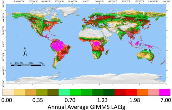
The NDVI3g data from July 1981 through December 2011 were used together with the 24 trained FFNN models to generate the corresponding LAI3g and FPAR3g data sets. These data sets have the same attributes as the input NDVI3g data: 1/12 degree spatial resolution and 15-day temporal frequency. Figure 1(a,b) shows color-coded maps of 30-year averages of annual mean LAI3g and FPAR3g. Figure 1(c,d) shows the time series of LAI3g anomalies for different latitudinal zones and land cover classes. The impact of Mount Pinatubo eruption in mid-1991 and significant orbit loss of NOAA 11 is clearly visible in the time series, especially in the tropics and in the forested regions of the globe. Data from year 2011 also exhibit significant positive anomalies, reasons for which are not known.
3. Assessment of LAI3g and FPAR3g Data Sets
The two objectives of our assessment of LAI3g and FPAR3g data sets are: (a) to provide uncertainty estimates through comparisons with field measurements and (b) to evaluate their suitability for use in research related to climate, hydrological, ecological, biogeochemical and crop yield models [3–17]. Analyses related to meet these objectives are described below.
3.1. Uncertainty Assessment
Providing uncertainty estimates for coarse resolution (1/12 degree) LAI3g and FPAR3g data sets is a challenging task as it requires a large number of comparable values derived from ground measurements. Further, the comparisons should be made for all major vegetation types and also cover the phenological cycle. Field campaigns are man-power intensive and therefore expensive. There have been very few suitable field campaigns before the NASA Earth Observing System (EOS) era, i.e., prior to year 2000. However, since the launch of Terra MODIS instrument, the scientific community has collaboratively developed a network of sites—e.g., BigFoot, AErosol RObotic NETwork, FLUXNET, EOS Land Validation Core Sites, VAlidation of Land European remote sensing Instruments, etc.—data from which have been used to validate moderate resolution (1 km) MODIS LAI and FPAR products [36,54–63]. In the process, the community has also developed common protocols for sampling the field sites and scaling methodologies that translate point-based field measurements of LAI and FPAR to the spatial scale of remotely-sensed products to facilitate accurate validation [35,64]. These efforts have resulted in establishing uncertainty estimates for the MODIS LAI and FPAR products [36].
Most of the field campaigns, and therefore, the validation efforts have been focused on the MODIS LAI product. The FPAR product is a by-product of the MODIS LAI algorithm and the underlying relationship between LAI and FPAR is based on the physics of radiative transfer [25]. The underlying relationship alleviates the need for independent and comprehensive validation of the FPAR3g product.
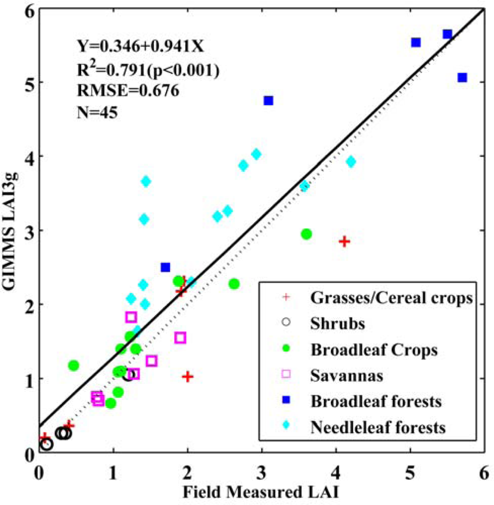
In this study, we selected sites with field measurements recorded over regions with more or less homogeneous groups of land cover classes, called biomes. Even then, a pixel-by-pixel comparison between LAI3g and field-measured LAI values scaled to LAI3g spatial resolution is not feasible because: (a) the spatial location of the satellite pixel contains uncertainties due to geo-location errors and pixel-shift errors resulting from the point spread function [65], and (b) point field measurements scaled to the resolution of the sensor necessarily involves uncertainty arising from the scaling methodology [55–59,64]. Therefore, the comparisons were performed on groups of pixels belonging to a particular biome and the assessment was based on the distribution properties of the respective values [36,57–59]. Specifically, the LAI3g data were compared to 45 sets of appropriately scaled field measurements from 29 sites listed in Table A4 of [40]. Monthly LAI3g values from nearby pixels of the same biome type were used for comparison purposes. The results indicate satisfactory agreement between LAI3g and scaled field measurements (p < 0.001; RMSE = 0.68 LAI) (Figure 2). This RMSE value may be taken as the uncertainty estimate of the LAI3g product, i.e., the average difference between LAI3g and ground truth value of LAI at the spatial resolution of the LAI3g product (1/12 degree).
3.2. Evaluation-Part 1: Comparison with the CYCLOPES LAI and FPAR Products
The goal of evaluation of LAI3g and FPAR3g products is to further imbue confidence in the use of these data sets in studies on monitoring of global vegetation dynamics and in modeling and applications research. One way to achieve this goal is to compare the new products (LAI3g and FPAR3g) with those already in use by the research community. The Carbon Cycle and Change in Land Observational Products from an Ensemble of Satellites (CYCLOPES) LAI and FPAR products (version 3.1) derived from the SPOT VEGETATION sensor are available at 1/112° Plate-Carrée spatial resolution and 10-day temporal frequency [66]. These products have reached a level of maturity comparable to the MODIS LAI and FPAR products [38]. We compared LAI3g and FPAR3g products with CYCLOPES LAI and FPAR products at global and site scale-information regarding the required preprocessing for these comparative analyses is given in Section S3. All data from the overlapping period between the two product sets, years 1999 to 2007, were used.
3.2.1. Global Scale Comparison
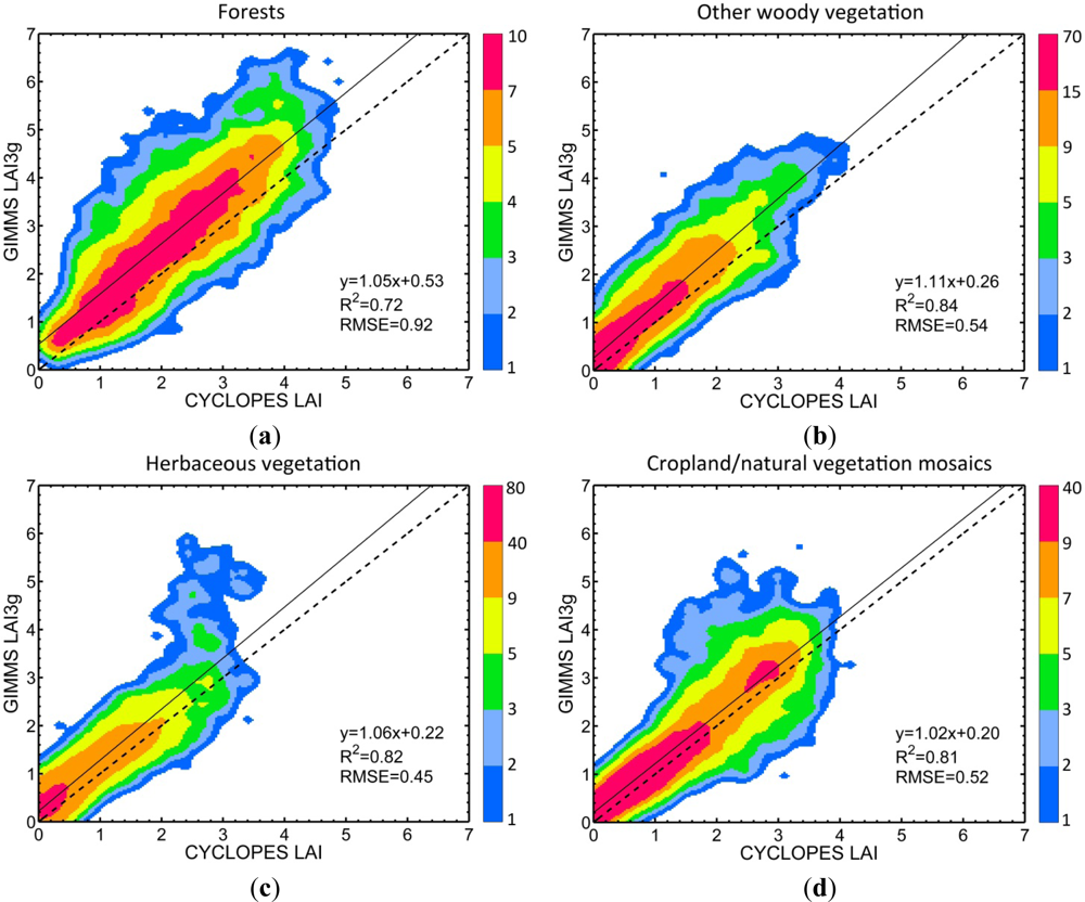
Figure 3 shows a comparison between LAI3g and corresponding CYCLOPES LAI values for four broad vegetation classes (Table S5) at the monthly time scale. The analysis suggests: (a) only in cropland/natural vegetation mosaics, the two products show satisfactory agreement (slope close to unity and minimal bias, (b) the slopes are considerably larger than unity in the case of forests and other woody vegetation classes, and (c) the slope is less than unity in the case of herbaceous vegetation. To investigate the general disagreement between the two LAI products, annual mean LAI from the two data sets for each of the IGBP land covers was evaluated (Table 1). Annual mean LAI3g is greater than the corresponding CYCLOPES LAI for all IGBP land covers with the exception of mixed forests and evergreen needleleaf forests. It is evident that the large disagreement in the case of forests (Figure 3(a)) is largely due to the Evergreen broadleaf forest cover type, which occupies 12.87% of the global total vegetated area (46.40% of the total forested area) and contributes to the maximum difference between the two data sets (1.03 in absolute LAI units). The CYCLOPES algorithm in general produces saturated LAI values at low values of LAI [38,39]. Results from a similar analysis between FPAR3g and CYCLOPES FPAR are shown in Figure S4. Besides, comparisons of multi-year average monthly values from CYCLOPES and our products are presented in Figure S5 (CYCLOPES LAI and LAI3g) and Figure S6 (CYCLOPES FPAR and FPAR3g).
3.2.2. Site Scale Comparison
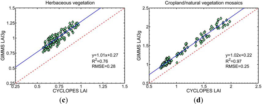
In this exercise, CYCLOPES LAI values from the Benchmark Land Multisite Analysis and Intercomparison of Products (BELMANIP) sites [67] were compared to corresponding LAI3g values. We chose sites representative of four broad vegetation classes (Table S5), each of areal extent 24 × 24 km2 (about 3 × 3 GIMMS pixels) and calculated monthly LAI values. Figure 4 shows comparison plots between the two products for 323 BELMANIP sites. In all cases, LAI3g and CYCLOPES LAI values lie in the proximity of the 1:1 line (slopes of 1.05, 1.11, 1.06 and 1.02, respectively, with corresponding offsets of 0.53, 0.26, 0.22 and 0.20). LAI3g explains 72.0%, 84.0%, 82.0% and 81.0% of the variability in the CYCLOPES LAI data and, on average, shows an error of 0.92, 0.54, 0.45 and 0.52 (in absolute LAI units). These results indicate that the agreement between the two data sets is better at the site scale than at global scale analysis, probably because of higher homogeneity of vegetation types at the sites. Results from a similar analysis between FPAR3g and CYCLOPES FPAR are shown in Figure S7.
3.3. Evaluation-Part 2: Comparison with Climatic Variables
A second method of evaluating LAI3g and FPAR3g data sets is to assess the degree of statistical association between these and climatic variables that limit plant growth [40,68]. Temperature, solar radiation and precipitation are the three key climatic variables that govern plant growth [69]. Vegetated areas showing temperature limitations to plant growth are mostly located in the northern latitudes, while areas strongly governed by precipitation are located in the tropical latitudes [69]. Therefore, examining the statistical association between covariations of LAI3g (and FPAR3g) and temperature in the northern latitudes and precipitation in the tropical regions provides an independent means of evaluating the new data sets. It is important to note that the LAI3g and FPAR3g data sets were generated without using climatic data—thus, the following statistical analyses are indeed independent evaluations of these data sets.
3.3.1. LAI3g Variation with Surface Temperature in the Northern Latitudes
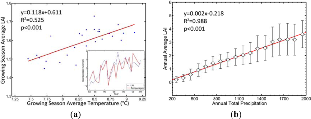
Vegetation photosynthetic activity and net primary production in the northern latitudes (50°N–90°N) have been reported to increase as a result of amplified surface warming during the period 1981 to 1999 [70–76]. We examine if the LAI3g and FPAR3g data sets reproduce and extend these results. First, we calculated the approximate growing season (May to September) averages of LAI3g and surface temperature for the region 50°N to 90°N for each year of the time series. All the vegetated pixels in the 50°N to 90°N latitudinal zone were area-weighted with the square root of pixel area to eliminate geometrical effects. Figure 5(a) shows a statistically significant relationship between the growing season averages of LAI3g and surface temperature (R2 = 0.525, p < 0.001). To reduce the likelihood of spurious correlation, we also analyzed the relationship between standardized anomalies of growing season averages of LAI3g and surface temperature [71] (Figure 5 inset). This analysis also resulted in a statistically significant correlation (R2 = 0.574, p < 0.001). These results thus not only reproduced previously published analyses but also show that the northern latitude greening trend is continuing as a result of continuing surface warming. Results from a similar analysis with FPAR3g data are shown in Figure S8(a).
3.3.2. LAI3g Variation with Precipitation in the Tropical Regions
Pixel-level data of annual total precipitation and annual mean LAI3g were averaged over the overlapping record length of these two variables (1982 to 2009) because precipitation, unlike temperature, exhibits greater spatial variability. The precipitation range, 200 mm/year to 2,000 mm/year, was divided into 18 intervals of width 100 mm/year. The mean and standard deviation of annual mean LAI3g of all pixels in each of these 18 precipitation intervals were evaluated. The resulting relationship, shown in Figure 5(b), indicates a statistically significant relationship (R2 = 0.988, p < 0.001). The dispersion in annual mean LAI3g (standard deviation plotted along the y-axis of Figure 5(b)) is greater than the dispersion in annual total precipitation (plotted along the x-axis of Figure 5(b)). This indicates that although precipitation may be the dominant control of plant growth in the tropical regions, other factors also play an important role [69]. Results from a similar analysis with FPAR3g are shown in Figure S8(b).
3.4. Evaluation-Part 3: Identifying Dominant Modes of Interannual Variability Using CCA
The correlations observed between LAI3g and temperature (Figure 5(a)) and between LAI3g and precipitation (Figure 5(b)) can be explained in terms of large-scale circulation anomalies, such as the EI Niño-Southern Oscillation (ENSO) and Arctic Oscillation (AO) [40,77]. The canonical correlation analysis (CCA) is well-suited to explore these connections as it seeks to estimate dominant and independent modes of co-variability between two sets of spatio-temporal variables [77], e.g., LAI3g and temperature.
The CCA is designed to select those temporal features in the LAI3g, or FPAR3g, fields that are best correlated with temporal features in springtime climatic variables such as temperature and/or precipitation. The methodology is illustrated here with LAI3g and “climatic variables” below denote either temperature or precipitation. Springtime (March to May) average values of LAI3g and the corresponding climatic variable for each pixel is denoted as a variable (for temperature, the total number of variables is the number of pixels in the latitudinal zone 10°N to 90°N; for precipitation, the total number of variables is the number of pixels in the latitudinal zone 40°S to 40°N). Further, each year is denoted as an observation, i.e., 28 observations for the overlapping time period—years 1982 to 2009. The anomaly fields of these variables for each pixel were weighted by the respective pixel area to avoid geometrical effects. Each set of variables was then transformed into principal components (PCs) using singular value decomposition. In each case, only the first six PCs were retained as they explain a large fraction of the variance in the input set of variables (LAI3g: 58.34%; FPAR3g: 56.55%; temperature: 69.88%; precipitation: 47.34%). PCs of LAI3g and climatic variables were input to the CCA. The CCA generates two canonical loading matrices, one for PCs of LAI3g and the other for PCs of the climatic variable. These are then used to construct canonical factors (CFs) from the original PC time series. This results in an eigenvalue matrix that depicts the correlation between the CFs. These eigenvalues (Table 2) suggest that the correlations between the first two CFs are reasonably high (r > 0.6), with the next two being moderate and the last two showing the weakest correlation. Table 2 indicates that: (1) there are strong correlations between CFs of LAI3g (and FPAR3g) and climatic variables; (2) the first two CFs are suitable to explore correlations with ENSO or AO.
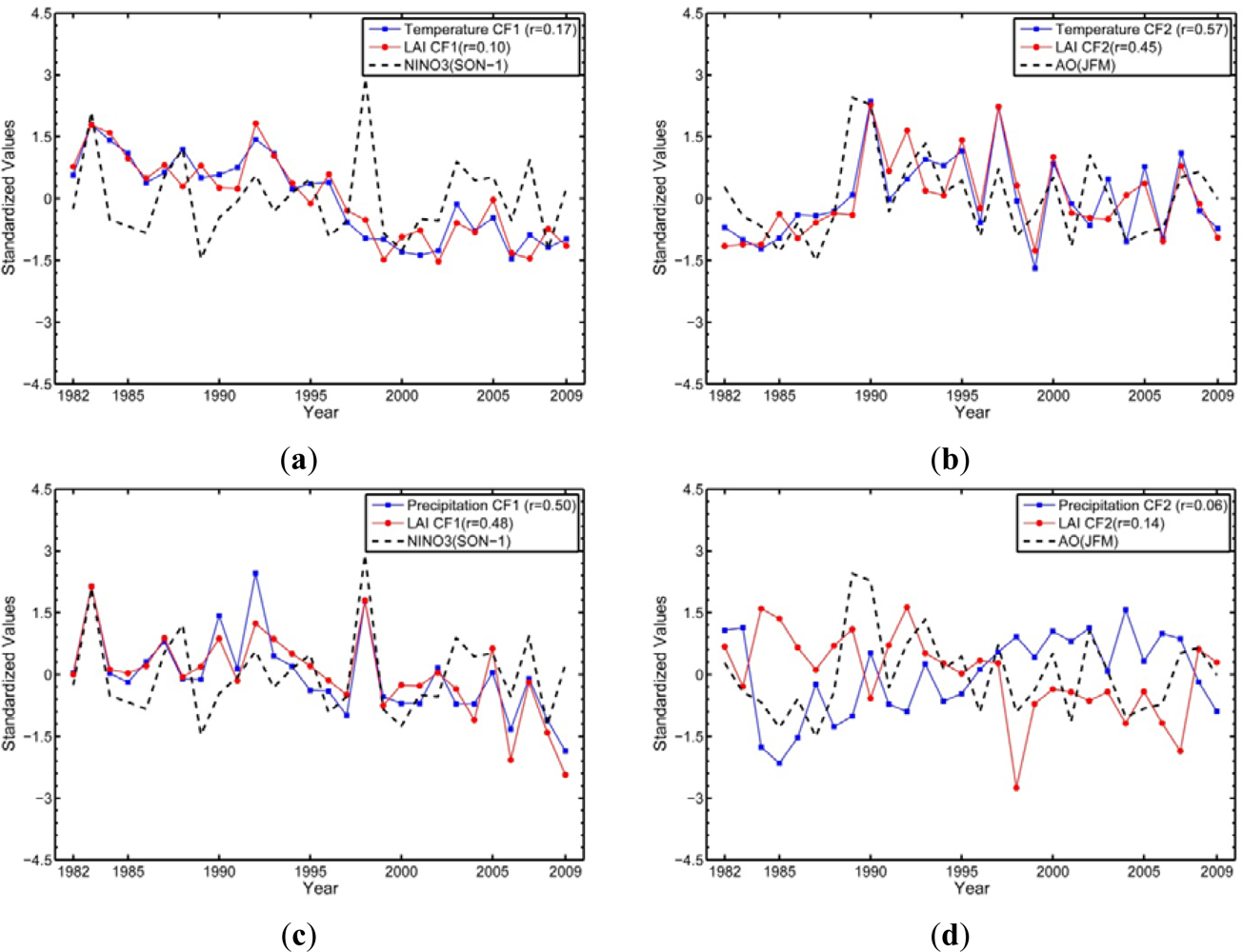
We used the September to November of the preceding year (SON-1) NINO3 index to represent ENSO and the January to March (JFM) average AO index because strong correlations between these indices with springtime climatic variables and NDVI were previously reported [77]. Figure 6(a) shows a low correlation between SON-1 NINO3 index and the first CFs of temperature and LAI3g (0.17 and 0.10, respectively). Compared to a previous study [77], the decline in correlation may be attributed to weak ENSO activity during the past decade [40]. We did observe a strong correlation between SON-1 NINO3 and the first CFs of temperature and LAI3g during the period 1982 to 1998 (0.66 and 0.67, respectively; figure not shown for brevity), consistent with results reported in [77]. Figure 6(b) shows a moderately strong correlation between JFM AO index and the second CFs of temperature and LAI3g (0.57 and 0.45, respectively), which is concordant with earlier studies [40,74].
Reasonable correlations were also observed between SON-1 NINO3 and the first CFs of precipitation and LAI3g (0.50 and 0.48, respectively; Figure 6(c)). This is consistent with previous reports of ENSO influence on interannual variability of tropical and extra-tropical precipitation [78]. The second CFs of precipitation and LAI3g are uncorrelated with the JFM AO index (Figure 6(d)), which is expected as the AO is not known to be a prime driver of precipitation in the 40°S to 40°N latitudinal zone [78]. The CCA was also performed on the FPAR3g data set. The results are similar to those reported here (Figure S9).
In summary, in the northern hemisphere in contrast to the period 1982 to 1998, ENSO driven linked variations between surface temperature and vegetation activity have weakened since 2000. In the tropical and extra-tropical regions, ENSO is still a strong driver of precipitation and vegetation variability. The influence of AO remains a factor in the interannual variability of temperature and vegetation activity in the northern hemisphere over the past three decades. These results reproduce published reports [40,77] but also reflect an updated picture. Additional analysis to assess the impact of loss of NOAA 11 orbit on these results is presented in Section S8.
4. Simple Case Study to Illustrate the Utility of LAI3g and FPAR3g Data Sets
Earth System Models (ESMs) are being used to project changes in different components of the climate system for various forcing scenarios [79]. The latest generation of ESMs include dynamic vegetation models that simulate global vegetation dynamics [80]. The confidence in model projections depends to a large degree on how well these models can simulate present-day climatic variables and several studies are geared to address this e.g., [81]. Here, we illustrate the utility of the newly developed LAI3g and FPAR3g data in the context of model evaluation with a simple case study where we compare LAI3g to model simulated values (the ESM output did not include the FPAR variable).
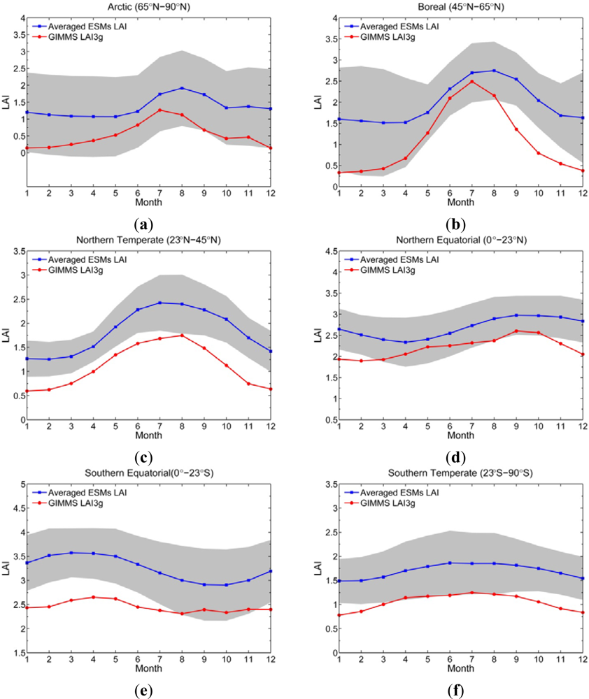
A strict comparison is difficult, if not impossible, because of the manner in which vegetation is modeled within the grid cell in each model and lack of this quantitative information. Comparisons at the grid cell-level are also difficult because of differences in spatial resolution of the ESMs (model grid cells varying from 0.938 to 3.75 degree) and satellite products (1/12 degree). Therefore, we performed comparisons at the zonal scale. We chose six latitudinal bands that may be approximately characterized as: (a) Arctic (65°N–90°N), (b) Boreal (45°N–65°N), (c) Northern Temperate (23°N–45°N), (d) Northern Equatorial (0°–23°N), (e) Southern Equatorial (0°–23°S) and (f) Southern Temperate (23°S–90°S). We evaluated the vegetated fraction of each model grid cell using the satellite-data based land cover map (Section S5.2) because of the difficulty of evaluating this quantity for each model grid cell and for all the 18 models used in this exercise.
Figure 7 shows the annual cycle of LAI3g and the ensemble mean LAI from 18 ESMs from the Coupled Model Intercomparison Project 5 (CMIP5) for the six latitudinal zones. The annual cycle of LAI3g is generally about the ensemble mean LAI minus one standard deviation of the ESM LAI. The bell-shaped patterns of LAI3g and the ensemble mean ESM LAI in the six latitudinal zones are approximately consistent. However, the timing of maximum ESM LAI is delayed by about 1 month relative to the LAI3g in the Arctic and Boreal zones. Comparison of MODIS LAI with the Community Land Model and Carbon-Nitrogen model simulations, also show that the timing of the maximum LAI lagged the observations by 1–2 months [82]. The fact that the ESMs are “greener” and their phenological cycle lags observations has important implications for simulated fluxes of energy, mass and momentum in the ESMs. Could it be that the dynamic vegetation models overestimate carbon fixation and/or allocation of biomass to leaves? This simple exercise illustrates the utility of satellite-data based products by highlighting an area of research that requires refinement in ESMs [83].
5. Concluding Remarks
The objective of this work was to generate, assess and document the utility of long-term (30-year) global LAI and FPAR data sets. The availability of a new improved NDVI data set from the NASA GIMMS research group, termed the third generation NDVI, or NDVI3g, and its overlap with the Terra MODIS LAI and FPAR products provided an opportunity to design and implement a neural network algorithm to generate the corresponding LAI3g and FPAR3g data sets with the following attributes: 15-day temporal frequency, 1/12 degree spatial resolution and temporal span of July 1981 to December 2011.
The suitability of LAI3g and FPAR3g data sets for monitoring and modeling global vegetation in the context of climate, biogeochemistry, eco-physiology, hydrology and agriculture [3–17] was comprehensively assessed. The LAI3g data were compared to 45 sets of appropriately scaled field measurements from 29 sites representative of all major biomes. The results indicated satisfactory agreement (p < 0.001; RMSE = 0.68 LAI). Compared to the widely-used alternate CYCLOPES LAI and FPAR products, the LAI3g and FPAR3g showed higher values, especially in forests—this is concordant with previous reports of CYCLOPES products as underestimates of ground truth values of LAI and FPAR. The LAI3g and FPAR3g products exhibited expected behavior with respect to their relationship with climatic variables: temperature in the northern latitudes and precipitation in the tropical regions. The interannual variability embedded in the LAI3g and FPAR3g data sets was evaluated for its relationship to large scale circulation anomalies that are dominant modes of interannul variability in climatic variables. The resulting strong correlations between the two dominant modes of variability in LAI3g (and FPAR3g) with ENSO and AO imbued confidence in the interannual variability of these data sets.
The utility of these data sets was documented by comparing the annual profile of LAI3g with profiles generated by 18 Earth System Models for various latitudinal zones. The results indicated that the models consistently overestimated satellite-based estimates of leaf area. Moreover, the models’ simulation of the seasonal cycle in the northern latitudes is at odds with the satellite product. Ground based studies have confirmed this inability of models to simulate the phenological cycle, which lends support to the seasonal cycle observed in the satellite-based LAI3g product. Finally, the LAI3g and FPAR3g data sets can be obtained freely from the NASA Earth Exchange (NEX) web site.
Supplementary Information
remotesensing-05-00927-s001.pdfAcknowledgments
We thank C. J. Tucker and J. Pinzon of NASA GSFC for making available the GIMMS NDVI3g data set. We also thank BELMANIP Project for providing the BELMANIP site for validation of our products. This study was partially funded by the China Scholarship Council and NASA Earth Science Division.
References
- Sellers, P.J.; Tucker, C.J.; Collatz, G.J.; Los, S.O.; Justice, C.O.; Dazlich, D.A.; Randall, D.A. A revised land surface parameterization (SiB2) for atmospheric GCMS. Part II: The generation of global fields of terrestrial biophysical parameters from satellite data. J. Climate 1996, 9, 706–737. [Google Scholar]
- Myneni, R.B.; Hoffman, S.; Knyazikhin, Y.; Privette, J.L.; Glassy, J.; Tian, Y.; Wang, Y.; Song, X.; Zhang, Y.; Smith, G.R.; Lotsch, A.; Friedl, M.; Morisette, J.T.; Votava, P.; Nemani, R.R.; Running, S.W. Global products of vegetation leaf area and fraction absorbed PAR from year one of MODIS data. Remote Sens. Environ 2002, 83, 214–231. [Google Scholar]
- Sellers, P.J.; Mintz, Y.; Sud, Y.C.; Dalcher, A. A simple biosphere model (sib) for use within general-circulation models. J. Atmos. Sci 1986, 43, 505–531. [Google Scholar]
- Melillo, J.M.; McGuire, A.D.; Kicklighter, D.W.; Moore, B.; Vorosmarty, C.J.; Schloss, A.L. Global climate change and terrestrial net primary production. Nature 1993, 363, 234–240. [Google Scholar]
- Ji, J. A climate-vegetation interaction model: Simulating physical and biological processes at the surface. J. Biogeogr 1995, 22, 445–451. [Google Scholar]
- Foley, J.A.; Prentice, I.C.; Ramankutty, N.; Levis, S.; Pollard, D.; Sitch, S.; Haxeltine, A. An integrated biosphere model of land surface processes, terrestrial carbon balance, and vegetation dynamics. Glob. Biogeochem. Cy 1996, 10, 603–628. [Google Scholar]
- Bonan, G.B.; Levis, S.; Sitch, S.; Vertenstein, M.; Oleson, K.W. A dynamic global vegetation model for use with climate models: Concepts and description of simulated vegetation dynamics. Glob. Change Biol 2003, 9, 1543–1566. [Google Scholar]
- Zhang, P.; Anderson, B.; Tan, B.; Huang, D.; Myneni, R. Potential monitoring of crop production using a satellite-based Climate-Variability Impact Index. Agr. Forest Meteorol 2005, 132, 344–358. [Google Scholar]
- Krinner, G.; Viovy, N.; de Noblet-Ducoudré, N.; Ogée, J.; Polcher, J.; Friedlingstein, P.; Ciais, P.; Sitch, S.; Prentice, I.C. A dynamic global vegetation model for studies of the coupled atmosphere-biosphere system. Glob. Biogeochem. Cy. 2005. [Google Scholar] [CrossRef]
- Demarty, J.; Chevallier, F.; Friend, A.D.; Viovy, N.; Piao, S.; Ciais, P. Assimilation of global MODIS leaf area index retrievals within a terrestrial biosphere model. Geophys. Res. Lett. 2007. [Google Scholar] [CrossRef]
- Wesely, M.L. Parameterization of surface resistances to gaseous dry deposition in regional-scale numerical models. Atmos. Environ 1989, 23, 1293–1304. [Google Scholar]
- Lu, L.; Shuttleworth, W.J. Incorporating NDVI-Derived LAI into the climate version of RAMS and its impact on regional climate. J. Hydrometeorol 2002, 3, 347–362. [Google Scholar]
- Brown, M.E.; Pinzon, J.E.; Didan, K.; Morisette, J.T.; Tucker, C.J. Evaluation of the consistency of long-term NDVI time series derived from AVHRR,SPOT-vegetation, SeaWiFS, MODIS, and Landsat ETM+ sensors. IEEE Trans. Geosci. Remote Sens 2006, 44, 1787–1793. [Google Scholar]
- Lathière, J.; Hauglustaine, D.A.; Friend, A.; de Noblet-Ducoudré, N.; Viovy, N.; Folberth, G. Impact of climate variability and land use changes on global biogenic volatile organic compound emissions. Atmos. Chem. Phys. Discuss 2005, 5, 10613–10656. [Google Scholar]
- Alessandri, A.; Gualdi, S.; Polcher, J.; Navarra, A. Effects of land surface-vegetation on the boreal summer surface climate of a GCM. J. Climate 2007, 20, 255–278. [Google Scholar]
- Piao, S.; Ciais, P.; Friedlingstein, P.; de Noblet-Ducoudré, N.; Cadule, P.; Viovy, N.; Wang, T. Spatiotemporal patterns of terrestrial carbon cycle during the 20th century. Glob. Biogeochem. Cy. 2009. [Google Scholar] [CrossRef]
- Anav, A.; Menut, L.; Khvorostyanov, D.; Viovy, N. A comparison of two canopy conductance parameterizations to quantify the interactions between surface ozone and vegetation over Europe. J. Geophys. Res. 2012. [Google Scholar] [CrossRef]
- Asrar, G.; Fuchs, M.; Kanemasu, E.T.; Hatfield, J.L. Estimating absorbed photosynthetic radiation and leaf area index from spectral reflectance in wheat. Agron. J 1984, 76, 300–306. [Google Scholar]
- Chen, J.M.; Pavlic, G.; Brown, L.; Cihlar, J.; Leblanc, S.G.; White, H.P.; Hall, R.J.; Peddle, D.R.; King, D.J.; Trofymow, J.A.; Swift, E.; van der Sanden, J.; Pellikka, P.K.E. Derivation and validation of Canada-wide coarse-resolution leaf area index maps using high-resolution satellite imagery and ground measurements. Remote Sens. Environ 2002, 80, 165–184. [Google Scholar]
- Myneni, R.B.; Ramakrishna, R.; Nemani, R.; Running, S.W. Estimation of global leaf area index and absorbed par using radiative transfer models. IEEE Trans. Geosci. Remote Sens 1997, 35, 1380–1393. [Google Scholar]
- Fassnacht, K.S.; Gower, S.T.; MacKenzie, M.D.; Nordheim, E.V.; Lillesand, T.M. Estimating the leaf area index of North Central Wisconsin forests using the Landsat Thematic Mapper. Remote Sens. Environ 1997, 61, 229–245. [Google Scholar]
- Colombo, R.; Bellingeri, D.; Fasolini, D.; Marino, C.M. Retrieval of leaf area index in different vegetation types using high resolution satellite data. Remote Sens. Environ 2003, 86, 120–131. [Google Scholar]
- Houborg, R.; Soegaard, H.; Boegh, E. Combining vegetation index and model inversion methods for the extraction of key vegetation biophysical parameters using Terra and Aqua MODIS reflectance data. Remote Sens. Environ 2007, 106, 39–58. [Google Scholar]
- Myneni, R.B.; Ross, J.; Asrar, G. A review on the theory of photon transport in leaf canopies. Agric. For. Meteorol 1989, 45, 1–153. [Google Scholar]
- Knyazikhin, Y.; Martonchik, J.V.; Myneni, R.B.; Diner, D.J.; Running, S.W. Synergistic algorithm for estimating vegetation canopy leaf area index and fraction of absorbed photosynthetically active radiation from MODIS and MISR data. J. Geophys. Res 1998, 103, 32257–32275. [Google Scholar]
- Combal, B.; Baret, F.; Weiss, M.; Trubuil, A.; Mace, D.; Pragnere, A.; Myneni, R.B.; Knyazikhin, Y.; Wang, L. Retrieval of canopy biophysical variables from bidirectional reflectance using prior information to solve the ill-posed inverse problem. Remote Sens. Environ 2002, 84, 1–15. [Google Scholar]
- Li, X.; Strahler, A.H. Geometric-optical bidirectional reflectance modeling of the discrete crown vegetation canopy—Effect of crown shape and mutual shadowing. IEEE Trans. Geosci. Remote Sens 1992, 30, 276–292. [Google Scholar]
- Li, X.; Strahler, A.H.; Woodcock, C.E. A hybrid geomeric optical-radiative transfer approach for modeling albedo and directional reflectance of discontinuous canopies. IEEE Trans. Geosci. Remote Sens 1995, 33, 446–480. [Google Scholar]
- Ross, J.K.; Marshak, A.L. Calculation of canopy bidirectional reflectance using the monte-carlo method. Remote Sens. Environ 1988, 24, 213–225. [Google Scholar]
- Lewis, P. Three-dimensional plant modelling for remote sensing simulation studies using the Botanical Plant Modelling System. Agron. Sustainable Dev 1999, 19, 185–210. [Google Scholar]
- Baret, F.; Clevers, J.G.P.W.; Steven, M.D. The robustness of canopy gap fraction estimates from red and near-infrared reflectances: A comparison of approaches. Remote Sens. Environ 1995, 54, 141–151. [Google Scholar]
- Kimes, D.S.; Ranson, K.J.; Sun, G. Inversion of a forest backscatter model using neural networks. Int. J. Remote Sens 1997, 18, 2181–2199. [Google Scholar]
- Weiss, M.; Baret, F.; Leroy, M.; Hautecœur, O.; Bacour, C.; Prévot, L.; Bruguier, N. Validation of neural net techniques to estimate canopy biophysical variables from remote sensing data. Agron. Sustain. Dev 2002, 22, 547–553. [Google Scholar]
- Fernandes, R.; Butson, C. A Landsat TM/ETM+ based accuracy assessment of leaf area index products for Canada derived from SPOT4/VGT data. Can. J. Remote Sens 2003, 29, 241–258. [Google Scholar]
- Morisette, J.T.; Baret, F.; Privette, J.L.; Myneni, R.B.; Nickeson, J.E.; Garrigues, S.; Shabanov, N.V.; Weiss, M.; Fernandes, R.A.; Leblanc, S.G.; et al. Validation of global moderate-resolution LAI products: A framework proposed within the CEOS land product validation subgroup. IEEE Trans. Geosci. Remote Sens 2006, 44, 1804–1817. [Google Scholar]
- Yang, W.; Tan, B.; Huang, D.; Rautiainen, M.; Shabanov, N.V.; Wang, Y.; Privette, J.L.; Huemmrich, K.F.; Fensholt, R.; Sandholt, I.; et al. MODIS leaf area index products: From validation to algorithm improvement. IEEE Trans. Geosci. Remote Sens 2006, 44, 1885–1898. [Google Scholar]
- Pisek, J.; Chen, J.M. Comparison and validation of MODIS and VEGETATION global LAI products over four BigFoot sites in North America. Remote Sens. Environ 2007, 109, 81–94. [Google Scholar]
- Weiss, M.; Baret, F.; Garrigues, S.; Lacaze, R. LAI and fAPAR CYCLOPES global products derived from VEGETATION. Part 2: Validation and comparison with MODIS collection 4 products. Remote Sens. Environ 2007, 110, 317–331. [Google Scholar]
- Garrigues, S.; Lacaze, R.; Baret, F.; Morisette, J.T.; Weiss, M.; Nickeson, J.E.; Fernandes, R.; Plummer, S.; Shabanov, N.V.; Myneni, R.B.; et al. Validation and intercomparison of global Leaf Area Index products derived from remote sensing data. J. Geophys. Res. 2008. [Google Scholar] [CrossRef]
- Ganguly, S.; Samanta, A.; Schull, M.A.; Shabanov, N.V.; Milesi, C.; Nemani, R.R.; Knyazikhin, Y.; Myneni, R.B. Generating vegetation leaf area index Earth system data record from multiple sensors. Part 2: Implementation, analysis and validation. Remote Sens. Environ 2008, 112, 4318–4332. [Google Scholar]
- Lee, T.E.; Miller, S.D.; Turk, F.J.; Schueler, C.; Julian, R.; Deyo, S.; Dills, P.; Wang, S. The NPOESS VIIRS day/night visible sensor. Bull. Am. Meteorol. Soc 2006, 87, 191–199. [Google Scholar]
- Lee, T.F.; Miller, S.D.; Schueler, C.; Miller, S. NASA MODIS previews NPOESS VIIRS capabilities. Weather Forecast 2006, 21, 649–655. [Google Scholar]
- Miller, S.D.; Schmidt, C.C.; Schmit, T.J.; Hillger, D.W. A case for natural colour imagery from geostationary satellites, and an approximation for the GOES-R ABI. Int. J. Remote Sens 2012, 33, 3999–4028. [Google Scholar]
- Wang, Q.; Wu, C.; Li, Q.; Li, J. Chinese HJ-1A/B satellites and data characteristics. Sci. China Ser. D 2010, 53, 51–57. [Google Scholar]
- Shimada, M.; Tadono, T.; Rosenqvist, A. Advanced Land Observing Satellite (ALOS) and monitoring global environmental change. Proc. IEEE 2010, 98, 780–799. [Google Scholar]
- Tucker, C.J.; Pinzon, J.E.; Brown, M.E.; Slayback, D.A.; Pak, E.W.; Mahoney, R.; Vermote, E.F.; El Saleous, N. An extended AVHRR 8-km NDVI dataset compatible with MODIS and SPOT vegetation NDVI data. Int. J. Remote Sens 2005, 26, 4485–4498. [Google Scholar]
- Yuan, H.; Dai, Y.; Xiao, Z.; Ji, D.; Shangguan, W. Reprocessing the MODIS Leaf Area Index products for land surface and climate modelling. Remote Sens. Environ 2011, 115, 1171–1187. [Google Scholar]
- Samanta, A.; Costa, M.H.; Nunes, E.L.; Vieira, S.A.; Xu, L.; Myneni, R.B. Comment on “Drought-induced reduction in global terrestrial net primary production from 2000 through 2009”. Science 2011, 333, 1093–1093. [Google Scholar]
- NASA. Goddard Space Flight Center. Available online: http://landval.gsfc.nasa.gov/ (accessed on 15 January 2013).
- Friedl, M.A.; McIver, D.K.; Hodges, J.C.F.; Zhang, X.Y.; Muchoney, D.; Strahler, A.H.; Woodcock, C.E.; Gopal, S.; Schneider, A.; Cooper, A.; et al. Global land cover mapping from MODIS: Algorithms and early results. Remote Sens. Environ 2002, 83, 287–302. [Google Scholar]
- Lotsch, A.; Tian, Y.; Friedl, M.A.; Myneni, R.B. Land cover mapping in support of LAI and FPAR retrievals from EOS-MODIS and MISR: Classification methods and sensitivities to errors. Int. J. Remote Sens 2003, 24, 1997–2016. [Google Scholar]
- Fang, H.; Li, W.; Myneni, R.B. The impact of potential land cover misclassification on MODIS Leaf Area Index (LAI) estimation: A statistical perspective. Remote Sens 2013, 5, 830–844. [Google Scholar]
- Heermann, P.D.; Khazenie, N. Classification of multispectral remote sensing data using a back-propagation neural network. IEEE Trans. Geosci. Remote Sens 1992, 30, 81–88. [Google Scholar]
- Privette, J.L.; Myneni, R.B.; Knyazikhin, Y.; Mukelabai, M.; Roberts, G.; Tian, Y.; Wang, Y.; Leblanc, S.G. Early spatial and temporal validation of MODIS LAI product in the Southern Africa Kalahari. Remote Sens. Environ 2002, 83, 232–243. [Google Scholar]
- Tian, Y.; Woodcock, C.E.; Wang, Y.; Privette, J.L.; Shabanov, N.V.; Zhou, L.; Zhang, Y.; Buermann, W.; Dong, J.; Veikkanen, B.; et al. Multiscale analysis and validation of the MODIS LAI product: I. Uncertainty assessment. Remote Sens. Environ 2002, 83, 414–430. [Google Scholar]
- Tian, Y.; Woodcock, C.E.; Wang, Y.; Privette, J.L.; Shabanov, N.V.; Zhou, L.; Zhang, Y.; Buermann, W.; Dong, J.; Veikkanen, B.; et al. Multiscale analysis and validation of the MODIS LAI product: II. Sampling strategy. Remote Sens. Environ 2002, 83, 431–441. [Google Scholar]
- Shabanov, N.V.; Wang, Y.; Buermann, W.; Dong, J.; Hoffman, S.; Smith, G.R.; Tian, Y.; Knyazikhin, Y.; Myneni, R.B. Effect of foliage spatial heterogeneity in the MODIS LAI and FPAR algorithm over broadleaf forests. Remote Sens. Environ 2003, 85, 410–423. [Google Scholar]
- Wang, Y.; Woodcock, C.E.; Buermann, W.; Stenberg, P.; Voipio, P.; Smolander, H.; Häme, T.; Tian, Y.; Hu, J.; Knyazikhin, Y.; Myneni, R.B. Evaluation of the MODIS LAI algorithm at a coniferous forest site in Finland. Remote Sens. Environ 2004, 91, 114–127. [Google Scholar]
- Tan, B.; Hu, J.N.; Huang, D.; Yang, W.Z.; Zhang, P.; Shabanov, N.V.; Knyazikhin, Y.; Nemani, R.R.; Myneni, R.B. Assessment of the broadleaf crops leaf area index product from the Terra MODIS instrument. Agric. For. Meteorol 2005, 135, 124–134. [Google Scholar]
- Cohen, W.B.; Maiersperger, T.K.; Turner, D.P.; Ritts, W.D.; Pflugmacher, D.; Kennedy, R.E.; Kirschbaum, A.; Running, S.W.; Costa, M.; Gower, S.T. MODIS land cover and LAI collection 4 product quality across nine sites in the western hemisphere. IEEE Trans. Geosci. Remote Sens 2006, 44, 1843–1857. [Google Scholar]
- Huang, D.; Yang, W.Z.; Tan, B.; Rautiainen, M.; Zhang, P.; Hu, J.N.; Shabanov, N.V.; Linder, S.; Knyazikhin, Y.; Myneni, R.B. The importance of measurement errors for deriving accurate reference leaf area index maps for validation of moderate-resolution satellite LAI products. IEEE Trans. Geosci. Remote Sens 2006, 44, 1866–1871. [Google Scholar]
- Sea, W.B.; Choler, P.; Beringer, J.; Weinmann, R.A.; Hutley, L.B.; Leuning, R. Documenting improvement in leaf area index estimates from MODIS using hemispherical photos for Australian savannas. Agric. For. Meteorol 2011, 151, 1453–1461. [Google Scholar]
- Kauwe, M.G.D.; Disney, M.I.; Quaife, T.; Lewis, P.; Williams, M. An assessment of the MODIS collection 5 leaf area index product for a region of mixed coniferous forest. Remote Sens. Environ 2011, 115, 767–780. [Google Scholar]
- Baret, F.; Morissette, J.T.; Fernandes, R.A.; Champeaux, J.L.; Myneni, R.B.; Chen, J.; Plummer, S.; Weiss, M.; Bacour, C.; Garrigues, S.; Nickeson, J.E. Evaluation of the representativeness of networks of sites for the global validation and intercomparison of land biophysical products: Proposition of the CEOS-BELMANIP. IEEE Trans. Geosci. Remote Sens 2006, 44, 1794–1803. [Google Scholar]
- Tan, B.; Woodcock, C.E.; Hu, J.; Zhang, P.; Ozdogan, M.; Huang, D.; Yang, W.; Knyazikhin, Y.; Myneni, R.B. The impact of gridding artifacts on the local spatial properties of MODIS data: Implications for validation, compositing, and band-to-band registration across resolutions. Remote Sens. Environ 2006, 105, 98–114. [Google Scholar]
- Baret, F.; Hagolle, O.; Geiger, B.; Bicheron, P.; Miras, B.; Huc, M.; Berthelot, B.; Niño, F.; Weiss, M.; Samain, O.; Roujean, J.L.; Leroy, M. LAI, fAPAR and fCover CYCLOPES global products derived from VEGETATION: Part 1: Principles of the algorithm. Remote Sens. Environ 2007, 110, 275–286. [Google Scholar]
- Baret, F.; Morissette, J.T.; Fernandes, R.A.; Champeaux, J.L.; Myneni, R.B.; Chen, J.; Plummer, S.; Weiss, M.; Bacour, C.; Garrigues, S.; Nickeson, J.E. Evaluation of the representativeness of networks of sites for the global validation and intercomparison of land biophysical products: Proposition of the CEOS-BELMANIP. IEEE Trans. Geosci. Remote Sens 2006, 44, 1794–1803. [Google Scholar]
- Buermann, W.; Wang, Y.; Dong, J.; Zhou, L.; Zeng, X.; Dickinson, R.E.; Potter, C.S.; Myneni, R.B. Analysis of a multiyear global vegetation leaf area index data set. J. Geophys. Res. 2002. [Google Scholar] [CrossRef]
- Churkina, G.; Running, S.W. Contrasting climatic controls on the estimated productivity of global terrestrial biomes. Ecosystems 1998, 1, 206–215. [Google Scholar]
- Myneni, R.B.; Keeling, C.D.; Tucker, C.J.; Asrar, G.; Nemani, R.R. Increased plant growth in the northern high latitudes from 1981 to 1991. Nature 1997, 386, 698–702. [Google Scholar]
- Zhou, L.; Tucker, C.J.; Kaufmann, R.K.; Slayback, D.; Shabanov, N.V.; Myneni, R.B. Variations in northern vegetation activity inferred from satellite data of vegetation index during 1981 to 1999. J. Geophys. Res 2001, 106, 20069–20083. [Google Scholar]
- Slayback, D.A.; Pinzon, J.E.; Los, S.O.; Tucker, C.J. Northern hemisphere photosynthetic trends 1982–99. Glob. Change Biol 2003, 9, 1–15. [Google Scholar]
- Nemani, R.R.; Keeling, C.D.; Hashimoto, H.; Jolly, W.M.; Piper, S.C.; Tucker, C.J.; Myneni, R.B.; Running, S.W. Climate-driven increases in global terrestrial net primary production from 1982 to 1999. Science 2003, 300, 1560–1563. [Google Scholar]
- Wang, X.; Piao, S.; Ciais, P.; Li, J.; Friedlingstein, P.; Koven, C.; Chen, A. Spring temperature change and its implication in the change of vegetation growth in North America from 1982 to 2006. PNAS 2011, 108, 1240–1245. [Google Scholar]
- Piao, S.; Wang, X.; Ciais, P.; Zhu, B.; Wang, T.; Liu, J. Changes in satellite-derived vegetation growth trend in temperate and boreal Eurasia from 1982 to 2006. Glob. Change Biol 2011, 17, 3228–3239. [Google Scholar]
- Mao, J.; Shi, X.; Thornton, P.E.; Piao, S.; Wang, X. Causes of spring vegetation growth trends in the northern mid-high latitudes from 1982 to 2004. Environ. Res. Lett. 2012. [Google Scholar] [CrossRef]
- Buermann, W.; Anderson, B.; Tucker, C.J.; Dickinson, R.E.; Lucht, W.; Potter, C.S.; Myneni, R.B. Interannual covariability in Northern Hemisphere air temperatures and greenness associated with El Niño-Southern Oscillation and the Arctic Oscillation. J. Geophys. Res 2003, 108, 4396. [Google Scholar]
- Dai, A.; Wigley, T.M.L. Global patterns of ENSO-induced precipitation. Geophys. Res. Lett 2000, 27, 1283–1286. [Google Scholar]
- Solomon, S.; Qin, D.; Manning, M.; Marquis, M.; Averyt, K.; Tignor, M.M.B.; Miller, H.L.; Chen, Z. Climate Change 2007: The Physical Science Basis; Cambridge University Press: New York, NY, USA, 2007; pp. 589–663. [Google Scholar]
- Taylor, K.E.; Stouffer, R.J.; Meehl, G.A. An overview of CMIP5 and the experiment design. Bull. Am. Meteorol. Soc 2011, 93, 485–498. [Google Scholar]
- Anav, A.; Friedlingstein, P.; Kidston, M.; Bopp, L.; Ciais, P.; Cox, P.; Jones, C.; Jung, M.; Myneni, R.B.; Zhu, Z. Evaluating the land and ocean components of the global carbon cycle in the CMIP5 Earth System Model. J. Climate 2013. in press. [Google Scholar]
- Randerson, J.T.; Hoffman, F.M.; Thornton, P.E.; Mahowald, N.M.; Lindsay, K.; Lee, Y.-H.; Nevison, C.D.; Doney, S.C.; Bonan, G.; Stöckli, R.; et al. Systematic assessment of terrestrial biogeochemistry in coupled climate-carbon models. Glob. Change Biol 2009, 15, 2462–2484. [Google Scholar]
- Richardson, A.D.; Anderson, R.S.; Arain, M.A.; Barr, A.G.; Bohrer, G.; Chen, G.; Chen, J.M.; Ciais, P.; Davis, K.J.; Desai, A.R.; et al. Terrestrial biosphere models need better representation of vegetation phenology: Results from the North American Carbon Program Site Synthesis. Glob. Change Biol 2012, 18, 566–584. [Google Scholar]


| IGBP Land Covers | GIMMS LAI3g | CYCLOPES LAI | Area Fraction (%) |
|---|---|---|---|
| Open shrublands | 0.56 | 0.45 | 19.18 |
| Grasslands | 0.6 | 0.45 | 13.89 |
| Evergreen broadleaf forests | 4.19 | 3.16 | 12.87 |
| Woody savannas | 1.72 | 1.44 | 12.29 |
| Croplands | 1.05 | 1.01 | 10.77 |
| Savannas | 1.51 | 1.17 | 8.1 |
| Cropland/natural vegetation mosaics | 1.89 | 1.59 | 6.71 |
| Mixed forests | 1.94 | 1.95 | 5.86 |
| Evergreen needleleaf forests | 1.43 | 1.69 | 5.35 |
| Deciduous needleleaf forests | 1.46 | 1.4 | 2.08 |
| Deciduous broadleaf forests | 2.34 | 1.91 | 1.58 |
| Closed shrublands | 0.81 | 0.57 | 1.33 |
| Canonical Factors | Eigenvalues | |||
|---|---|---|---|---|
| LAI3g/TEMP | LAI/3gPRECIP | FPAR3g/TEMP | FPAR3g/PRECIP | |
| 1 | 0.93 | 0.90 | 0.93 | 0.86 |
| 2 | 0.86 | 0.63 | 0.91 | 0.72 |
| 3 | 0.69 | 0.49 | 0.80 | 0.49 |
| 4 | 0.57 | 0.40 | 0.78 | 0.47 |
| 5 | 0.33 | 0.29 | 0.54 | 0.12 |
| 6 | 0.02 | 0.09 | 0.00 | 0.04 |
Share and Cite
Zhu, Z.; Bi, J.; Pan, Y.; Ganguly, S.; Anav, A.; Xu, L.; Samanta, A.; Piao, S.; Nemani, R.R.; Myneni, R.B. Global Data Sets of Vegetation Leaf Area Index (LAI)3g and Fraction of Photosynthetically Active Radiation (FPAR)3g Derived from Global Inventory Modeling and Mapping Studies (GIMMS) Normalized Difference Vegetation Index (NDVI3g) for the Period 1981 to 2011. Remote Sens. 2013, 5, 927-948. https://doi.org/10.3390/rs5020927
Zhu Z, Bi J, Pan Y, Ganguly S, Anav A, Xu L, Samanta A, Piao S, Nemani RR, Myneni RB. Global Data Sets of Vegetation Leaf Area Index (LAI)3g and Fraction of Photosynthetically Active Radiation (FPAR)3g Derived from Global Inventory Modeling and Mapping Studies (GIMMS) Normalized Difference Vegetation Index (NDVI3g) for the Period 1981 to 2011. Remote Sensing. 2013; 5(2):927-948. https://doi.org/10.3390/rs5020927
Chicago/Turabian StyleZhu, Zaichun, Jian Bi, Yaozhong Pan, Sangram Ganguly, Alessandro Anav, Liang Xu, Arindam Samanta, Shilong Piao, Ramakrishna R. Nemani, and Ranga B. Myneni. 2013. "Global Data Sets of Vegetation Leaf Area Index (LAI)3g and Fraction of Photosynthetically Active Radiation (FPAR)3g Derived from Global Inventory Modeling and Mapping Studies (GIMMS) Normalized Difference Vegetation Index (NDVI3g) for the Period 1981 to 2011" Remote Sensing 5, no. 2: 927-948. https://doi.org/10.3390/rs5020927