
Influence of Wave-Induced Radiation Stress on Upper-Layer Ocean Temperature during Typhoons
by
 ,
,
Qianhui Wang
,
Jian Shi
*,
Jingmin Xia
,
Kaifeng Han
,
Wenbin Xiao
,
Wenjing Zhang
,
Haodi Wang
and
Jialei Lv
College of Meteorology and Oceanography, National University of Defense and Technology, Changsha 410073, China
*
Author to whom correspondence should be addressed.
Remote Sens. 2023, 15(9), 2442; https://doi.org/10.3390/rs15092442
Submission received: 17 April 2023
/
Revised: 26 April 2023
/
Accepted: 2 May 2023
/
Published: 6 May 2023
(This article belongs to the Special Issue Advances in the Ocean Surface Dynamics: Ocean Waves, Wind, and Air-Sea Interaction - in Memory of Professor Shengchang Wen)
Abstract
:Radiation stress is defined as the excess momentum caused by ocean waves, which exerts an indispensable impact on the upper-layer ocean conditions as waves pass by. Previous research concentrated on sea surface cooling caused by typhoons. In this paper, we investigated the effect of wave-induced radiation stress on upper-layer ocean temperature (including sea surface temperature (SST) and mixed-layer temperature) under typhoon conditions, as well as the effect of radiation stress on the surface current field. The FVCOM-SWAVE model, which is based on the SWAN model, is used to simulate the response of upper-layer ocean temperature to radiation stress. The simulated results, when validated with Jason-3 satellite and ARGO data, could reproduce the observed phenomenon well in general. Compared to simulations without radiation stress, the bias in the SST results is reduced by about 1 °C if the radiation stress term is taken into account. The mixed-layer depth temperature is expected to be simulated more accurately, with a root mean square error (RMSE) of less than 1.63 °C and a correlation coefficient (COR) of about 0.94. Results show that wave-induced radiation stress enhances the surface current and causes certain deviations to the right so that the upper water diverges and upwelling increases, resulting in a decrease in SST. When the influence of double typhoons is considered, the airflow of LEKIMA(L) rotates from the northwest toward KROSA (R), limiting the development of significant wave height (SWH) and reducing the cooling range. As a result, the present study is of tremendous importance in precisely forecasting the ocean state of the western North Pacific (WNP).
1. Introduction
Typhoons in the ocean are generally accompanied by strong winds and large swells over the sea surface, resulting in marine disasters and severe coastal damage [1]. As a result of violent exchanges of momentum and heat in the upper-layer ocean, Typhoons induce extraordinary climatic changes, including sea surface temperature (SST) cooling and sea level reduction [2,3]. When a typhoon passes over the sea surface, its strong wind stress will provoke significant current shear at the bottom of the mixed layer, leading to intense shear instability and mixing. These mixing forces subsurface cold water to the sea surface and prompts SST cooling [4,5]. The cooling on the right-hand side (RHS) of the typhoon track is normally greater than that on the left. This is due to the local wind rotation direction on the RHS of the track being consistent with the rotation direction of typhoon-generated near-inertial currents (clockwise in the Northern Hemisphere), enhancing vertical mixing of the upper-layer ocean [4,6]. Generally, three processes are mainly responsible for typhoon-induced SST cooling: upwelling, vertical mixing, and air–sea heat exchange [4,7,8,9]. According to a heat budget study, vertical mixing is the primary cause of the reduction in ocean surface temperature [10,11,12].
Moreover, the magnitude and range of typhoon-induced SST cooling are basically dependent on both the typhoon parameters and the pre-typhoon thermal condition. Typical typhoon parameters include typhoon intensity, translation speed, and typhoon size. Previous research has found that a strong, slow-moving typhoon tends to produce a larger magnitude of SST cooling [5,13]. Changes in thermal structure in the upper ocean have a significant impact on the magnitude of SST cooling by changing the Mixed Layer Depth (MLD) and the vertical temperature gradient below the mixed layer. Nevertheless, ocean waves are not explicitly included in ocean models in most cases, leading to overestimated SST and an underestimated MLD [14,15].
Waves and currents are important participants in ocean dynamics that interact with one another. Although waves occur at the sea surface, their influence can reach a certain depth via vertical mixings and modify the thermal conditions of the upper ocean. These will further alter the surface wind and cause surface current variations. For example, when waves reach large ocean current systems such as the Gulf Stream and Kuroshio, they refract and diffract, causing variations in wave height, wave direction, and wave amplitude. Meanwhile, structural changes in the ocean current field will affect the velocity and direction of the ocean wave. [16]. Furthermore, the interaction of ocean waves and currents exerts a significant impact on other ocean phenomena, such as storm surges, rip currents, nearshore circulation, and heat waves. Therefore, it is necessary to have a further understanding of the dynamic and thermal characteristics of these wave-current interaction processes.
In general, wave-current interaction includes depth-dependent wave radiation stress terms, Stokes drift, vertical transfer of wave-generated pressure, wave dissipation, etc. [17]. Longuet-Higgins and Stewart first proposed the concept of radiation stress in the 1960s, which was defined as the excess current of momentum due to the existence of waves [18]. Its influence is equivalent to the normal stress and shear stress acting on the water body below the surface wave, inducing the rise and fall of the average water level and the generation of circulations since then [11,14]. After that, many researchers supplied the concept of radiation stress and obtained its various mathematical expressions by deriving the current velocity and wave pressure formulas according to different wave theories. James [19] assumed the wave motion was slow and dependent on depth in the fracture zone. The hyperbolic approximation of elliptic cosine waves was used in shallow water, and the third-order Stokes wave theory was applied to calculate the variation of radiation stress along the shoreward direction. Feddersen [20] further considered the influence of wave direction spectrum distribution on radiation stress, which is realized by calculating the wave radiation stress using the Pierson–Moscowitz (PM) spectrum and comparing the results with the classical theoretical values. Zheng et al. [21] proposed a new method to calculate radiation stress by linking wave radiation stress with the variables to be solved in the parabolic gentle slope equation. Mellor et al. [17] added the wave-induced three-dimensional radiation stress to the momentum and energy conservation equation and provided numerical methods which apply to wave-current interaction processes.
Furthermore, it is supposed to improve the prediction level of oceanographic elements by taking radiation stress into consideration [22]. Radiation stress can change the direction of the current field regularly through the transfer of the momentum flux [18]. Meanwhile, the change of current field diverges the upper water and causes upwelling, which could also enhance the sea-surface cooling effect through vertical mixing when radiation stress is included [23,24]. This phenomenon also exerts a significant impact on typhoon thermohaline response. The wave radiation stress can significantly enhance surface current and induce certain rightward deviations, which does not fully conform with the rule of Ekman drift theory [25]. It is found that radiation stress can also be caused by internal waves. The interaction between waves and currents is more important than that on the surface [18]. It is also found that the current field has a significant influence on significant wave height (SWH). If the current direction is opposite to the wave direction, the SWH increases and vice versa.
The east coast of mainland China is close to the western North Pacific (WNP) area, which contains four of China’s major marginal seas. As a result, precisely forecasting WNP sea conditions is commercially important. It is of great significance to investigate the wave-current interaction in the WNP under typhoon conditions. FVCOM, an unstructured-grid ocean model, was shown to be capable of simulating three-dimensional circulation and storm surges in coastal regions [26,27,28].
The Jason-3 satellite altimeter and ARGO buoy data are used in the present study to investigate the response of upper-layer temperature to wave-induced radiation stress during typhoons, as well as the surface ocean circulation and wave distribution characteristics. The study area, data of Typhoons L and R, coupled model setup, and verification data are all briefly discussed in Section 1. Section 2 provides detailed simulation results and upper-ocean temperature variation considering radiation stress. The variation of the upper-layer flow field is discussed in Section 3. Conclusions are given in Section 4.
2. Materials and Methods
2.1. Study Area and Datasets
The simulated area extends from 97°E to 155°E and from 1°N to 57°N in the WNP and East China Sea. The Philippines Islands, Taiwan Islands, and Japan Islands are all included in the calculation area.
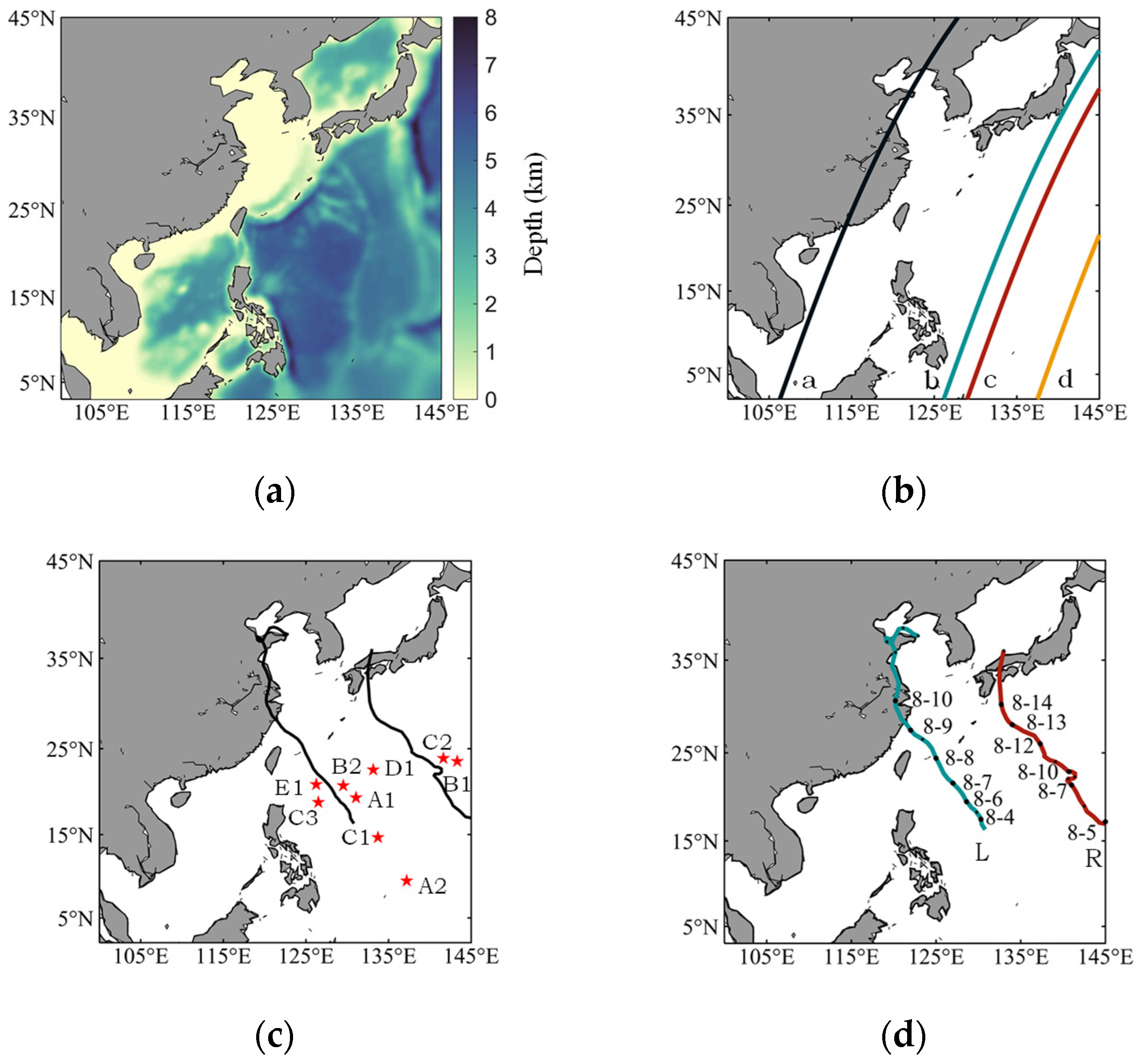
The topographic data used in the model is the ETOPO1 data from NOAA National Centers (http://www.ngdc.noaa.gov/mgg/global/global.html, accessed on 1 May 2023) with a resolution of 1′ × 1′ (Figure 1a). The wind data are from the ERA-interim project of the European Centre for Mesoscale Weather Prediction (ECMWF), which started in 2006 and is based on the original project ERA-40, using improved atmospheric models and a four-dimensional variational assimilation method, with wind field resolution of 0.125° × 0.125°, 6 hourly (https://www.ecmwf.int/, accessed on 1 May 2023). Daily averaged heat flux data (shortwave radiation, longwave radiation, sensible heat flux, and latent heat flux) are taken from the National Centers for Environment Prediction (NCEP) (https://downloads.psl.noaa.gov/Datasets/ncep.reanalysis/surface_gauss/, accessed on 1 May 2023), with a resolution of 1.875° × 1.875°, 6 hourly. The initial temperature, salinity fields, and lateral boundary conditions are derived from the Hybrid Coordinate Ocean Model (HYCOM) data (https://www.hycom.org/, accessed on 1 May 2023) with a resolution of 0.08° × 0.08°. The above data need to be interpolated to the unstructured triangular mesh used by the Finite Volume Coastal Ocean Model (FVCOM) and converted to a mesh data form that can be recognized by FVCOM during numerical simulation. To verify the accuracy of wind and wave simulations, the Jason-3 satellite altimeters in the Ku band are used. The Jason-3 satellite altimeters in the Ku band are used to validate the accuracy of wind and wave models. The Jason-3 altimeters have a revisit period of around 10 days at orbit 254 per period and measure sea-level variations in the world oceans with very high accuracy (0.033 m). The orbit diagram is shown in Figure 1b, whose approximate times correspond to a, b, c, and d is around 1600 UTC (coordinated universal time) 5 August, 1500 UTC 6 August, 1300 UTC 8 August, and 1400 UTC 9 August, respectively. The precision of the Ku band data is stated in the specification to be 0.001 m, and the observation result is better than that of the c band; so, the SWH of the Ku band inversion is used as the verification data in this work. The temperature profiles are based on the ARGO floats derived from the International Argo Program and the national programs (http://www.argo.org.cn, accessed on 1 May 2023). In this experiment, 9 buoys (A1–E1) at various latitudes along the typhoon path are selected (Figure 1c). Argo floats are a group of active floats providing temperature profiles from the surface to a depth of 2000 m.
2.2. Typhoons LEKIMA and KROSA
Typhoon LEKIMA (L) was the sixth most powerful typhoon to make landfall in China’s coastal areas since 1949. It originated over the sea east of the Philippines at 1400 UTC 4 August and strengthened into a strong tropical storm at 0200 UTC 6 August. It moved to the WNP with a maximum velocity of 62 m/s and a minimum pressure of 915 hPa. On the night of 8 August, L attained its maximum intensity as it swept across the sea near the island of Miyakojima. L made landfall as a super typhoon near China’s coast at 0200 UTC 10 August, with a maximum speed of 52 m/s.
Typhoon KROSA (R) developed soon after Typhoon L. R developed in the Philippines at 2000 UTC 5 August, northeast of Manila, and strengthened into a severe tropical storm on the morning of 7 August. It further developed into a strong typhoon at 1400 UTC 8 August, moving to the northeast, with a maximum wind speed of 42 m/s and a minimum pressure of 960 hPa. It gradually turned northwest on 10 August, with little change in velocity intensity, and then made landfall in southern Japan on 15 August.
Typhoons L and R were typical double typhoons, which both had a high landing intensity, and extremely wide range of wind impact with long duration, causing severe wind and rain impacts in the Bohai Sea. The eastern Philippines and the vicinity of Miyakojima Island both had small and medium-sized river floods, flash floods and landslides with different degrees. Typhoons L and R passed over multiple Argo buoy floats in the WNP from 6 August to 10 August (Figure 1c). It is supposed to simulate at 1200 UTC 5 August in the WNP to analyze the effect of wave-induced radiation stress. The tracks of double typhoons are illustrated in Figure 1d.
2.3. The Modeling System
2.3.1. Ocean Model FVCOM
FVCOM is a triangular-grid, 3-D, primitive equation ocean model [29]. As one of the popular ocean circulation models, FVCOM has been extensively applied to coastal and estuarine environments [30,31,32]. The model uses the finite volume method, which combines the geometric flexibility of a finite-element method and the simple discrete calculation of the finite difference method. The numerical model used in this study consists of seven primitive ocean governing equations (three for momentum, one for incompressible continuity, two for temperature and salinity, and one for density). The irregular bottom slope uses -coordinate transformation; and the horizontal grids comprise unstructured triangular cells [33]. (The -coordinate transformation is defined as , where varies from −1 at the bottom to 0 at the surface).
2.3.2. Wave Model FVCOM-SWAVE
FVCOM-SWAVE is a triangular-grid, SWAN-based phase-averaged wave model [34]. The wave action balance equation is employed to calculate the wave spectrum evolution in temporal, geographical and spectral spaces [35,36]. The module is based on the third-generation wave model, converting the structured-grid surface wave model Simulating Waves Nearshore (SWAN) into an unstructured-grid finite-volume version (FVCOM-SWAVE), whose version shares a grid with the FVCOM circulation model. Despite using different calculation approaches, the finite-volume advection scheme used in SWAVE shared the same numerical accuracy as the third-order finite-difference method used in SWAN [35]. Its governing equation for wave action density is written as follows:
where is time; is the wave action density spectrum; is the relative wave direction from the geographical East; is the relative wave frequency, and are the wave propagation velocities in spectral space, is group velocity, and is current vector. The factor in Equation (1) is critical in the quantification of wave shortening/lengthening. The wave action density in Equation (1) is solved numerically by three integral steps: variation of action density spectrum in spectral space, frequency, and direction, respectively; wave propagation in geographic space; and the growth, transfer, and decay of waves [37].
The term on the RHS of Equation (1) includes the change of wave action in the temporal, geographical, and spectral domain, which can be described as follows:
where is the function for wind-induced wave growth, is the nonlinear transfer of wave energy due to triadic three-wave interactions and four-wave interactions. The last three terms on RHS of Equation (2) represent dissipation due to white capping, shallow-water depth-induced breaking, and bottom friction, respectively.
The three-wave interactions transfer energy from lower frequencies to higher ones in shallow water. The SWAVE model calculates the directionally decoupled propagation of energy over the spectrum from lower to higher frequencies using the Lumped Triad Approximation (LTA) formulation [37]. Bi-phase of the self-interactions of the peak frequency components is used in the LTA formulation to express the three-wave interaction, which is parameterized in terms of Ursell Number with the following formulation [37]:
where is the bi-phase of wave, is the Ursell number, is the zero-moment wave height, and represents the mean absolute wave period.
2.3.3. Model Coupling and Wave-Current Interaction
To increase the accuracy of wave-current interactions, the FVCOM and SWAVE models exchange information at each wave time step (wave time step is always the product of current time step and an integer number) [38]. SWAVE calculates the change of wave action in temporal space from null initialization condition and determines the wave parameters, such as SWH, wave direction and wavelength. Wave-induced radiation stress is calculated by SWAVE and delivered to FVCOM. Momentum and continuity equations are used to compute current and surface elevation fields and added radiation stress gradients.
Current and surface elevation fields are computed by momentum and continuity equations in FVCOM in the next step and added radiation stress gradient terms [39].
The excess flux of momentum in the surf zone transferring from the wave model to the circulation model is expressed as radiation stress gradients. The and components of the radiation stress , , , are given as follows:
where , , and represents the residual momentum current acting in the direction perpendicular to the -axis plane and in the direction perpendicular to the -axis plane and in the direction perpendicular to the -axis plane, respectively [18]. is the wave energy (). , , and are SWH, wave number, wave number in the x direction, and wave number in the y direction, respectively. , , , and are the vertical structure functions given as follows:
where η is sea-surface elevation, is mean water depth, η is the total water depth.
2.3.4. Numerical Model Setup
An unstructured triangular horizontal grid (Figure S1) is used in this experiment, consisting of 26,073 compute nodes and 50,244 triangular grids. The land boundary, island boundary, and ocean open boundary are all taken into account. Sponge boundary conditions are used on open boundaries. The model adopts -coordinate in the vertical direction with 40 layers. Time steps of the internal and external mode are 30 and 3 s, respectively; and the output time interval is 60 min. The external mode is two-dimensional, calculating the average velocity and water level, while the internal mode is three-dimensional, calculating turbulent kinetic energy, three-dimensional velocity, temperature, salinity, and other physical quantities. The internal and external modes have the same transport property.
2.3.5. Sensitivity Experiments
As mentioned above, it is expected to reduce SST by taking radiation stress into account. In order to quantify the contribution of the radiation stress to SST cooling, we performed two sensitivity experiments with and without radiation stress gradient. First, the control experiment was based on the original condition, which was labeled Ur without radiation stress. Second, we artificially added radiation stress gradient to momentum equations, denoted as the Ar. The simulating time is from 1200 UTC 4 August to 0000 UTC 12 August.
The accuracy of the simulated results is measured by peak error (), mean absolute error (), mean absolute percentage Error (), model evaluation coefficient (), root mean square error (), and correlation coefficient () between simulated and observational values. These are the statistical measures:
where and , respectively, the represent observational values and simulated values. and represent the average of the observational values and simulated values, respectively. represents the number of data points (Table 1).
3. Results and Discussion
3.1. Wave Simulation Results
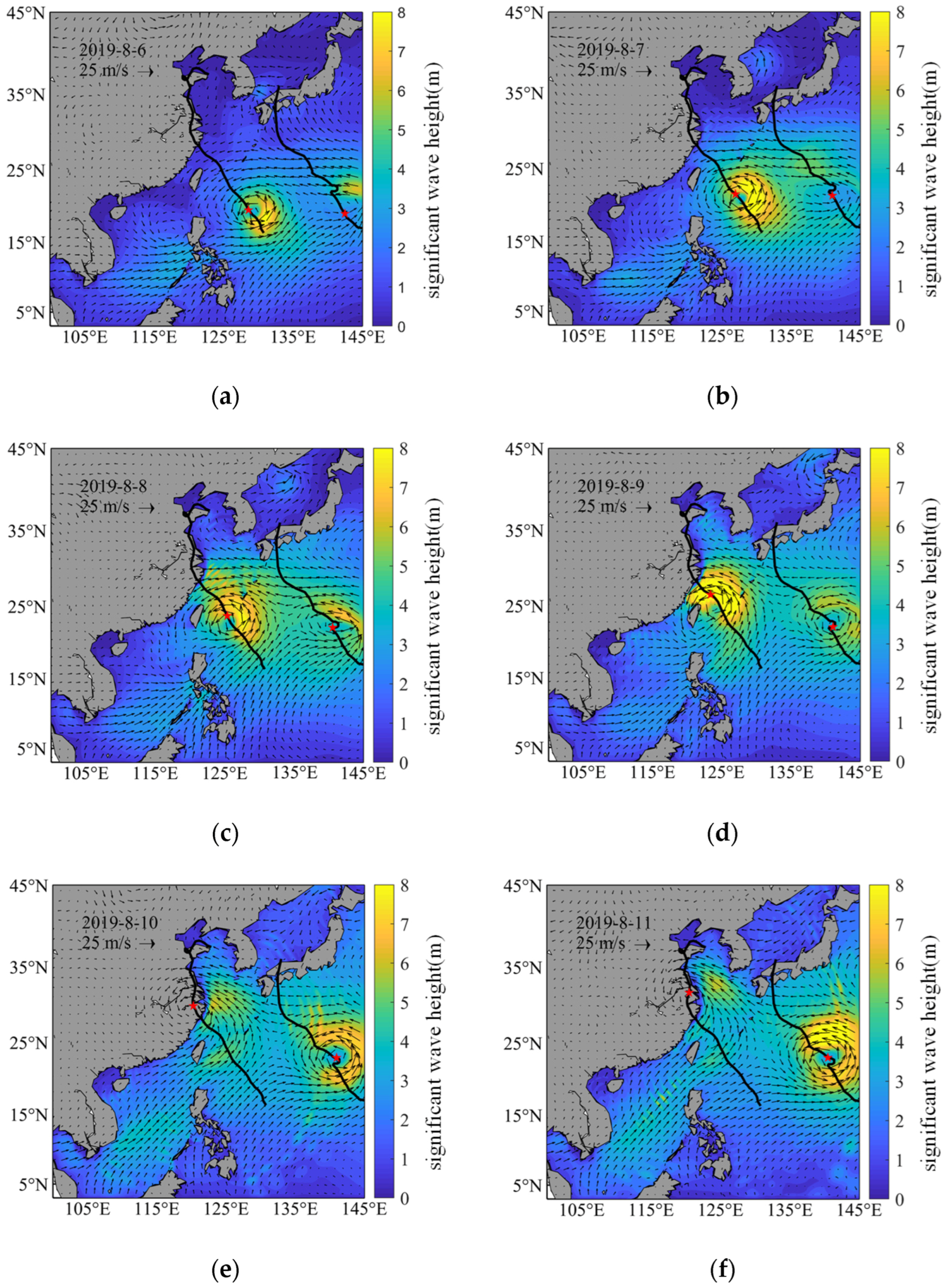
The SWHs simulated by FVCOM-SWAVE are shown in Figure 2. Accompanied by strong typhoon waves, oceanographic elements are affected during typhoons. The SWH in the typhoon area was much higher than that in the non-typhoon area. On the whole, the SWH in the non-typhoon area was roughly less than 1.5 m, while the SWH in the typhoon area could reach 8 m with a maximum value of 9.3 m.
The results of the numerical study proved the obvious right bias in SWH generated by these two typhoons. On 4 August, Typhoon L started from the east of the Philippines and moved to the WNP. The affected sea area grew significantly due to violent wind fields. Typhoon L upgraded to a severe tropical storm on 6 August, and visible typhoon waves emerged on the right rear side of the typhoon, with a maximum SWH of roughly 7 m. L grew into a super typhoon on 8 August, as the storm continued to intensify. Typhoon L produced a maximum SWH around 8.7 m, while Typhoon R produced just 4.3 m due to the deep water depth and the absence of complex islands. According to the ECMWF wind data, the wind speed on the right-hand side (RHS) of the path was much higher than that on the left-hand side (LHS), which is consistent with the theory that strong winds cause massive waves. When L made landfall in Zhejiang Province as a super typhoon on 10 August, the maximum wind speed reached 52 m/s. However, the area of ocean waves became smaller due to the effect of topography. Despite the severe winds, the maximum SWH generated by Typhoon L was just about 5 m.
The wind speed on RHS of the typhoon’s moving direction was superimposed with its moving speed, leading to a higher SWH in the right half circle than that in the left one. This is consistent with our results. Until 11 August, L had almost no impact on the sea surface, while the range of SWH generated by R further increased with the maximum SWH of about 9.3 m at the time.
Under the mutual impact of the two wind fields, airflow from L entered the R wind field from the northwest via rotation, while airflow from R entered the L wind field from the southeast through rotation. The densities of the L and R wind fields were greater on the right side, resulting in the appearance of maximum wind speed. Wave height correlates strongly with wind speed, so the maximum SWH created by the double typhoons was greater than that on the RHS of the track. According to Figure 2a,b, during the early stages of Typhoon R, the cyclonic character of Typhoon R was weakened due to the effect of the wind field of L, resulting in a small SWH.
On 8 August, as Typhoon L gradually moved away, the SWH created by R began to gradually increase, and the waves increased gradually. Taking into account the topographic obstruction and shallower water depth, Typhoon R’s maximum wind speed emerged on the RHS of the typhoon route on 11 August, and the maximum SWH was higher than that on the RHS of the path, demonstrating the normal rightward deviation of typhoon waves.
The spread of typhoon waves is demonstrated to be related to a variety of characteristics, including typhoon severity, movement path, and topography. The interaction between the wind fields of the double typhoons affected the distribution of maximum wind speed and typhoon waves. By analyzing the characteristics of the double typhoons, the airflow of L rotated from the northwest toward R, restricting the development of SWH (Figure 2) and reducing the cooling range of SST (Figure 2).
3.2. Simulated Currents
3.2.1. Simulated Surface Currents
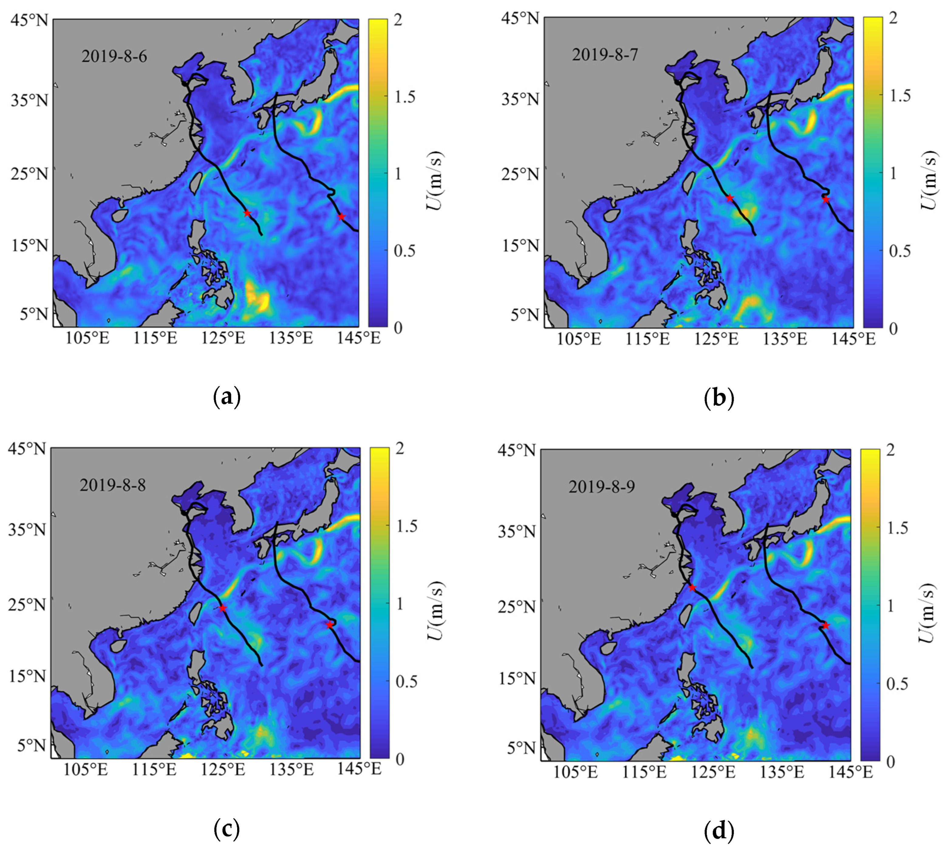
The surface current distribution in the WNP simulated by FVCOM is shown in Figure 3. The current velocity U was uniform during typhoons, and the average current velocity U was less than 0.6 m/s. The seasonal fluctuation of the seawater density field (particularly the surface layer) causes seasonal variation in the surface-layer current system. The current velocity of the Kuroshio is around 0.4–1.2 m/s. The speed of the current around the typhoon path increased during the typhoons. The velocity increase caused by L was larger than that caused by R.
3.2.2. Simulated SST
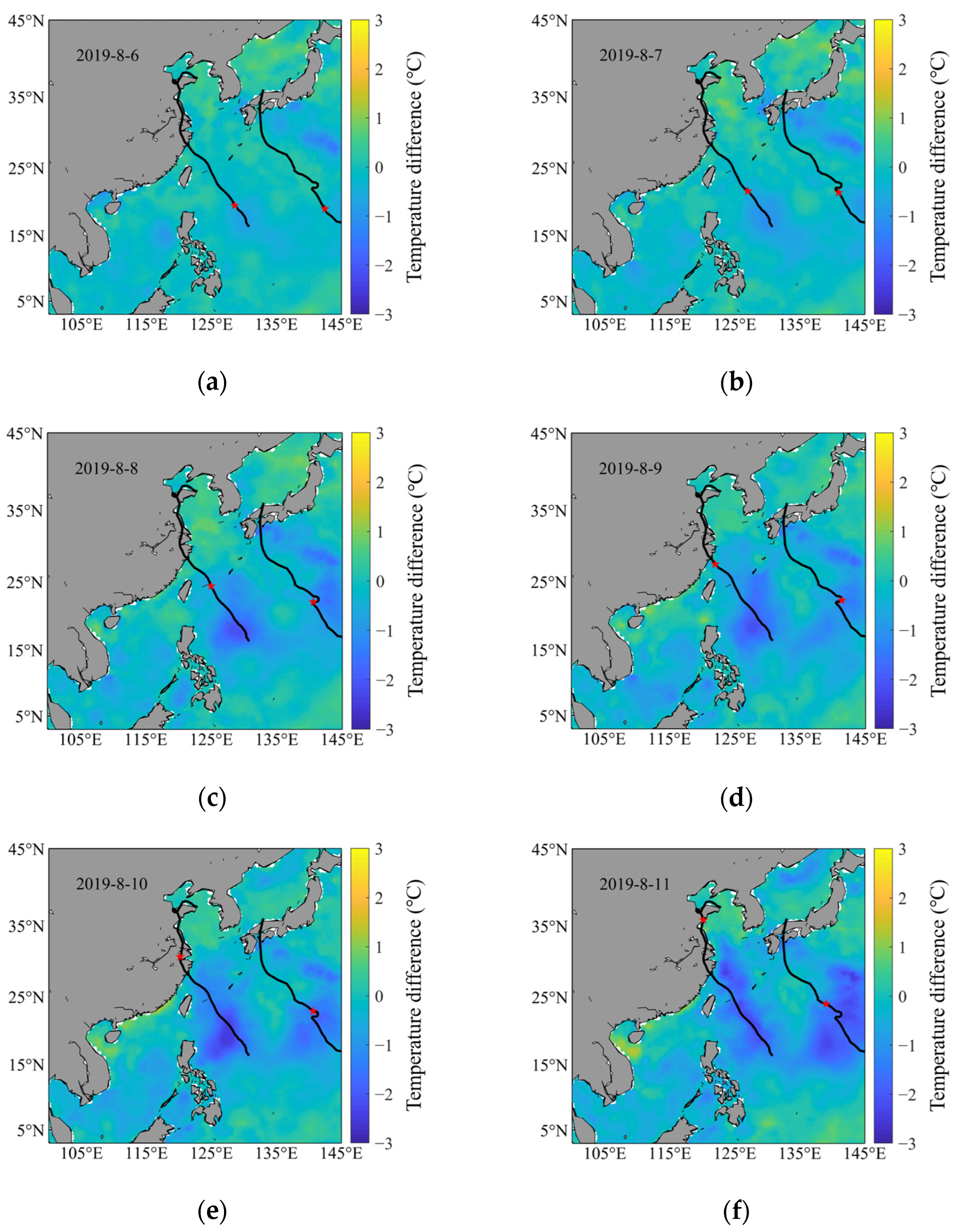
The SST on 4 August was taken as the initial temperature, and the differences between SST in different periods and the initial temperature are illustrated in Figure 4. Strong mixing and upwelling caused by typhoons lead to decreased SST. Furthermore, the highest SST reduction occurred 1–2 d after the appearance of maximum typhoon wind speed. In the early stage of typhoons, the intensity of typhoon L, the wind field, the ocean wave field, and the current field were relatively weak. The typhoons induced little upwelling and divergence, and the effect of decreasing SST was not obvious. On the night of 8 August, L progressively passed through Misako Island with intensity, reaching a peak with a large area of cooling range of 1.5 °C. However, the maximum SST reduction occurred on 10 August, two days after the maximum wind speed. The temperature dropped about 2.5 °C with the diffusion direction shifted from southwest to northwest.
To sum up, the double typhoons exerted a significant effect on SST reduction, but the cooling was delayed by about two days. Before 8 August, Typhoon R moved relatively quickly with relatively weak intensity, with no evident surface cooling area. On 8 August, it abruptly slowed down with increased intensity. A large cooling zone developed when R turned right, and the temperature dropped about 1.8 °C. When R turned left on 10 August, the cooling range expanded, but its cooling intensity weakened to 1 °C. After that, R moved toward Japanese Island with a maximum temperature drop of around 3 °C on 11 August.
It was demonstrated that oceanic responses during the two sudden-turning stages of R were much more remarkable than those in its straight-moving stage (Figure 4). Theoretically, the temperature drop generated by Typhoon R should be less than that of L. However, the slow movement and sudden turning stage result in a wider maximum cooling range and area.
During the sudden-turning phase of Typhoon R, the track change extends the typhoon’s forcing period on the ocean, resulting in a significant cooling zone, which is in agreement with Zhang [40]. Compared to the cooling effect caused by the two sudden turns, the first cooling was more intense. Since the turning angle and typhoon intensity were substantially smaller than those of the first stage, the SST cooling was minimal during the second stage.
3.3. Verification of Simulated SWH
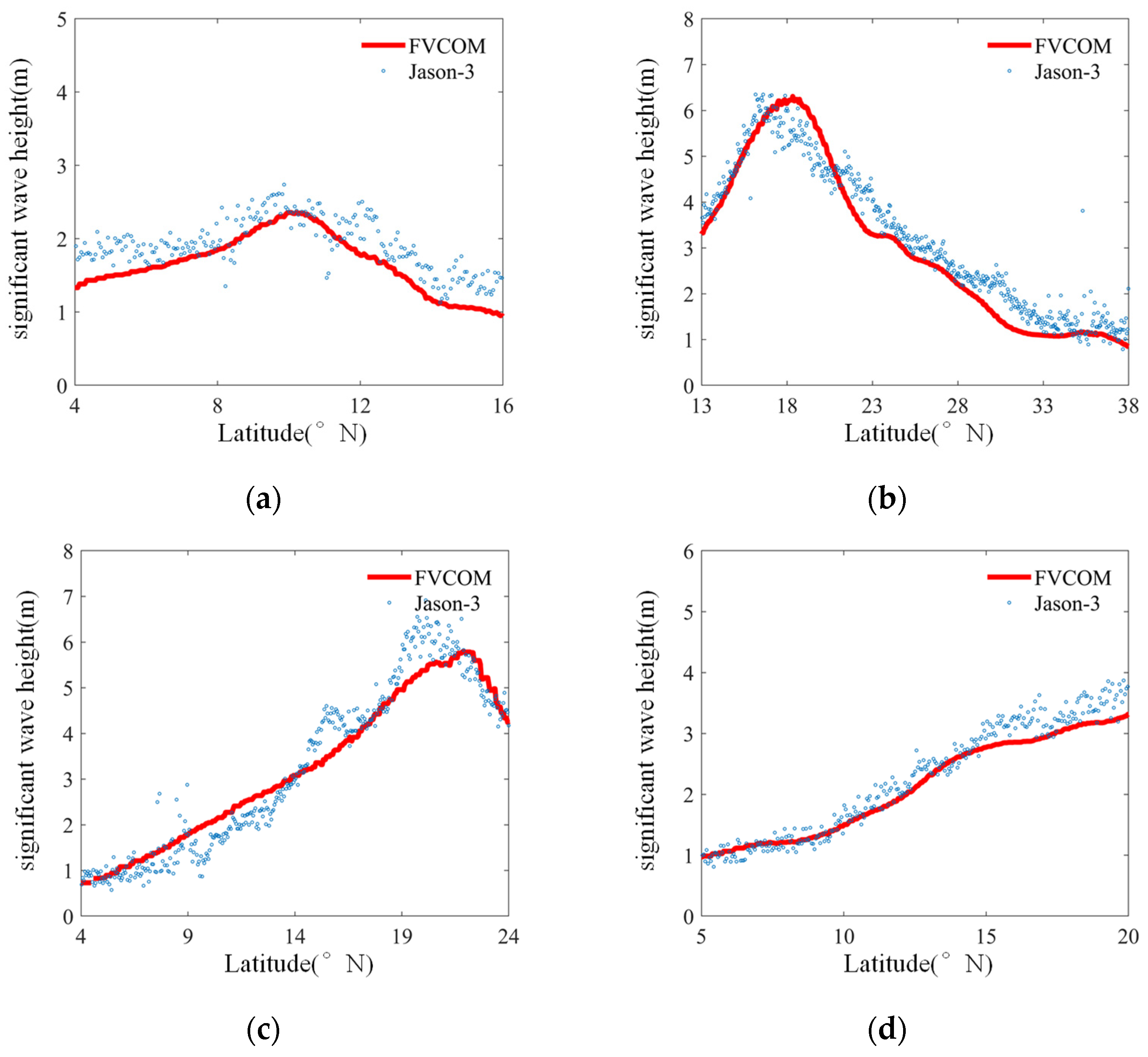
The SWH is supposed to be a vital standard to measure wave growth since typhoons are accompanied by waves. To demonstrate the accuracy and reliability of the simulation results, Jason-3 satellite data were used to verify the SWH during the typhoons from multiple spatial and temporal perspectives (Figure 5).
Table 1 displays the , , and of simulated values and observational values during the typhoons. It is indicated that the simulated results of FVCOM are consistent with Jason-3 satellite data and the simulated value is slightly lower than the measured one. The is in the range of 0.238 to 0.534 m. All of the values are greater than 0.843, showing a significant correlation between the simulated and measured SWH values.
3.4. Simulated Temperature
3.4.1. The Simulated Results of SST
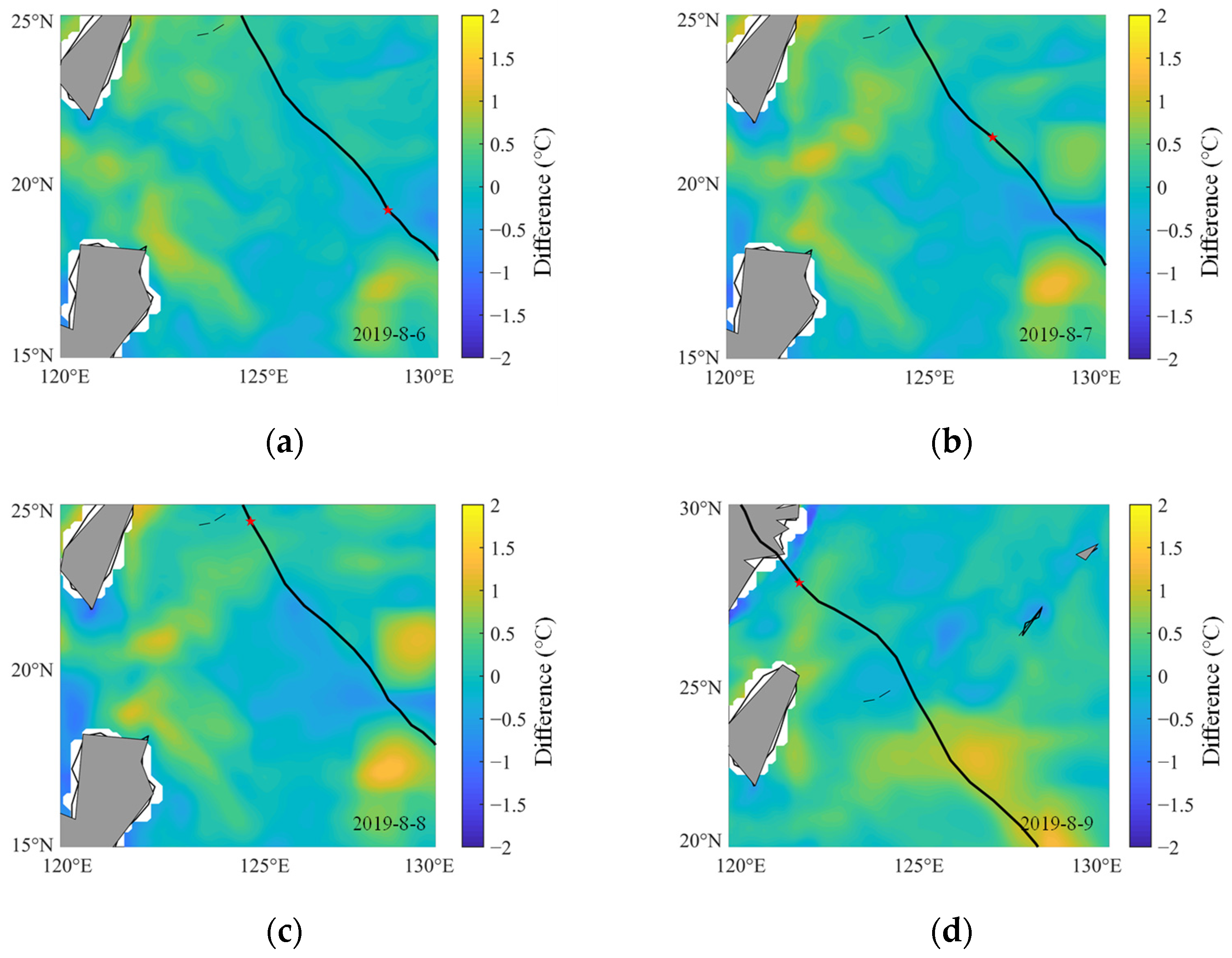
As a violent expression of the processes between air and sea, ocean waves promote not only the heat radiation flux from the ocean to the atmosphere but also the turbulent action of the upper-layer ocean, indirectly reducing the temperature of the upper-layer ocean. The Optimum Interpolation Sea Surface Temperature (OISST) product was used to validate the simulated SST without radiation stress (Figure 6). If the radiation stress is not considered, the simulated SST values in most sea areas are higher, with an inaccuracy of 1.5 °C.
To investigate the impact of wave-induced radiation stress on SST, we compare SST simulations with and without wave-induced stress (Figure 7). The simulation temperature at a depth of about 1 m is used for SST. The improvement due to including radiation stress is defined as follows:
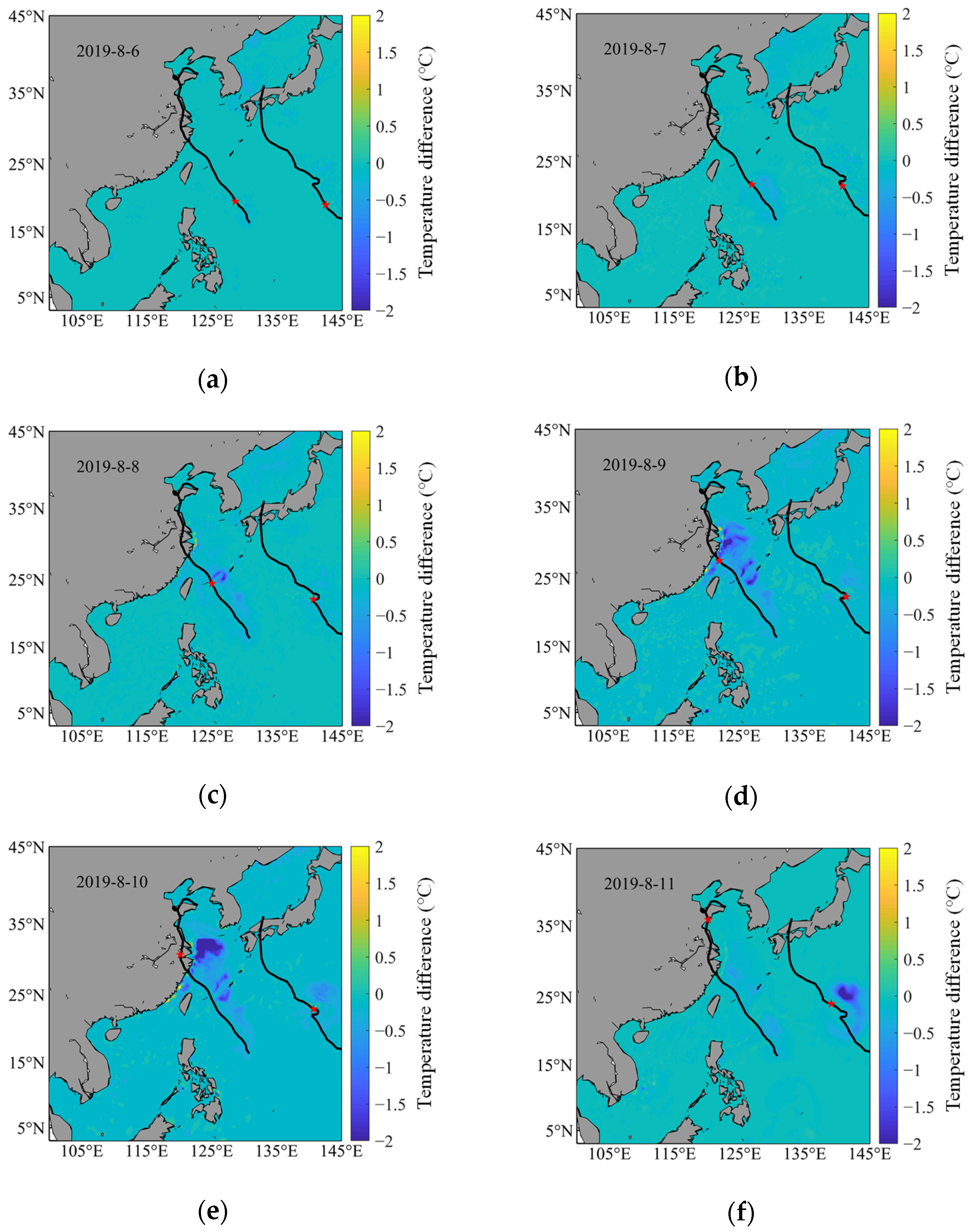
Here, and represent SST with and without considering the radiation, respectively. The spatial distribution of α shows that the SST is reduced by taking radiation stress into account (Figure 7). The area of temperature decrease is consistent with the SWH distribution in Figure 2. Furthermore, the magnitude of sea surface cooling increases with the increase in wave intensity.
The intensity of wind and wave field were small in the early stage of Typhoon L, which contributed to slight cooling caused by wave-induced radiation stress. On 9 August, radiation stress became stronger with the growth of the typhoon; and it strengthened the exchange of upper and lower water bodies, resulting in a large cooling of 2.5 °C in the area (Figure 7d). The cooling area also gradually expanded and spread along the entire path which changed with the movement of the typhoon. On 10 August, a significant cooling occurred in the northwest direction of the East China Sea with a maximum cooling of 3.7 °C (Figure 7e). The cooling caused by Typhoon R followed the same trend.
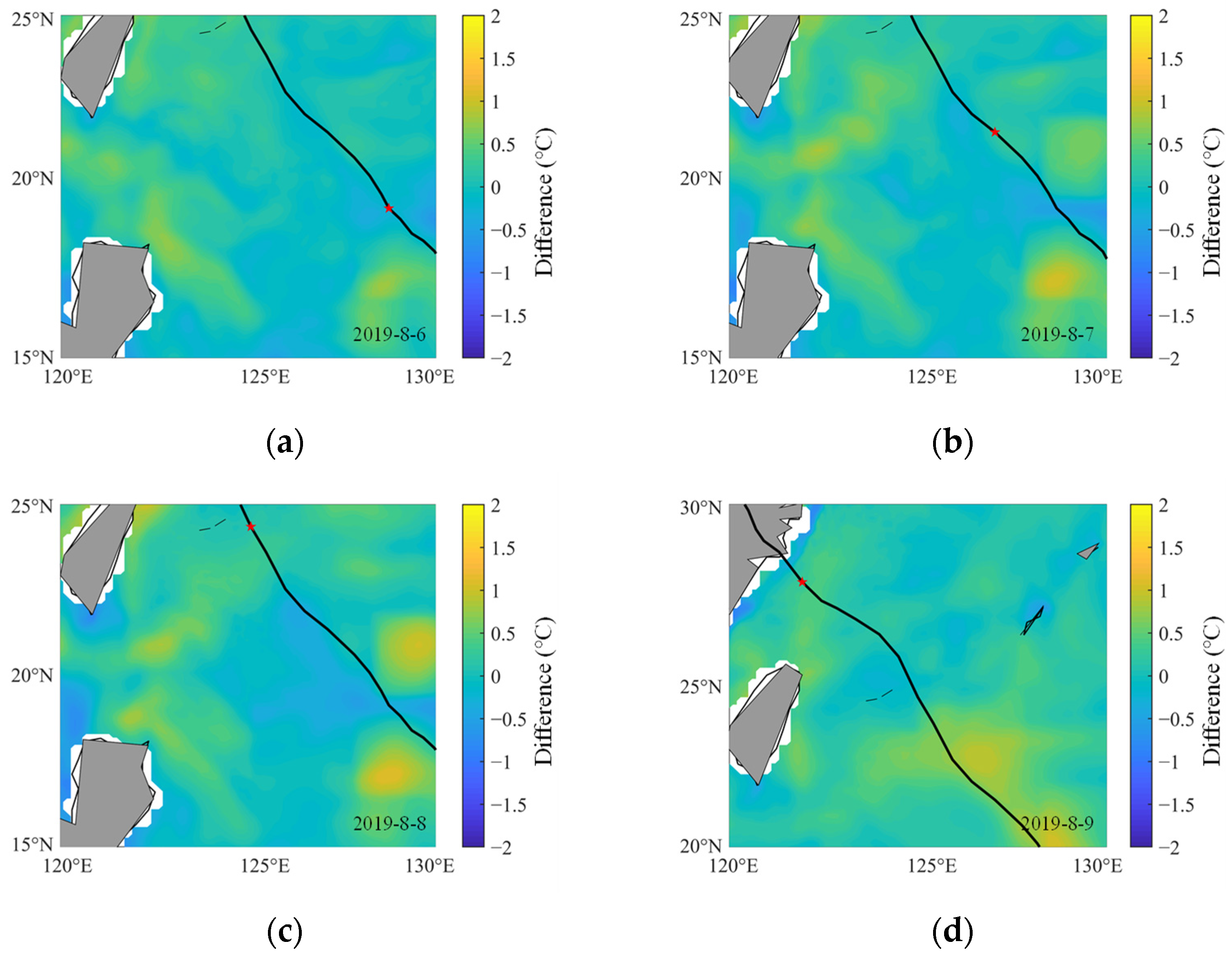
The error between the simulated SST with the radiation stress and OISST data is calculated (Figure 8). According to Figure 6, Figure 7 and Figure 8, the simulated SST shows better agreement with observations by taking the radiation stress into account. Most ocean areas have a simulation error of less than 0.5 °C, and the simulated SST is closer to the OISST data. Radiation stress can routinely shift the direction of the current field regularly through the transfer of the momentum flux. Meanwhile, changes in the current field diverge the upper water and cause upwelling [23]. The upwelling enhances the convection in the upper mixed layer, which affects the surface water, and the enhancement of convection between the upper and lower layers of seawater cools the SST [41].
The surface current field changed under the action of typhoon waves, bringing about water divergence and upwelling. The upper layer of water is displaced, resulting in a lower sea temperature. However, it takes about 1–2 days for the adjustment of SST, which fit the result of D’asaro E [42]. In other words, the change of SST caused by waves will lag about 1–2 days behind the transit of the typhoon. It is shown that typhoons affect the ocean surface not only through wind stress but also through wave action, such as wave-induced radiation stress.
3.4.2. The simulated Results of Mixed-Layer Temperature
Previous research focused on the sea surface cooling caused by typhoons [2,3,4,5,6]. Our study further provides the influence of wave-induced radiation stress on mixed-layer temperature under typhoons condition, as well as the effect of radiation stress on the surface current field. When the double typhoons passed over the study area, , , , and of the simulated subsurface ocean temperature were calculated. Table 2 shows the maximum was 1.63 °C. The average with radiation stress was 0.21 °C smaller than the average without radiation stress. The values of these results were all above 0.88, and the average of the simulated result with radiation stress increased by 0.02. The average of the simulated result with radiation stress rose by 0.03. Similar results can be obtained from simulated temperatures below the mixed layer with and without radiation stress.
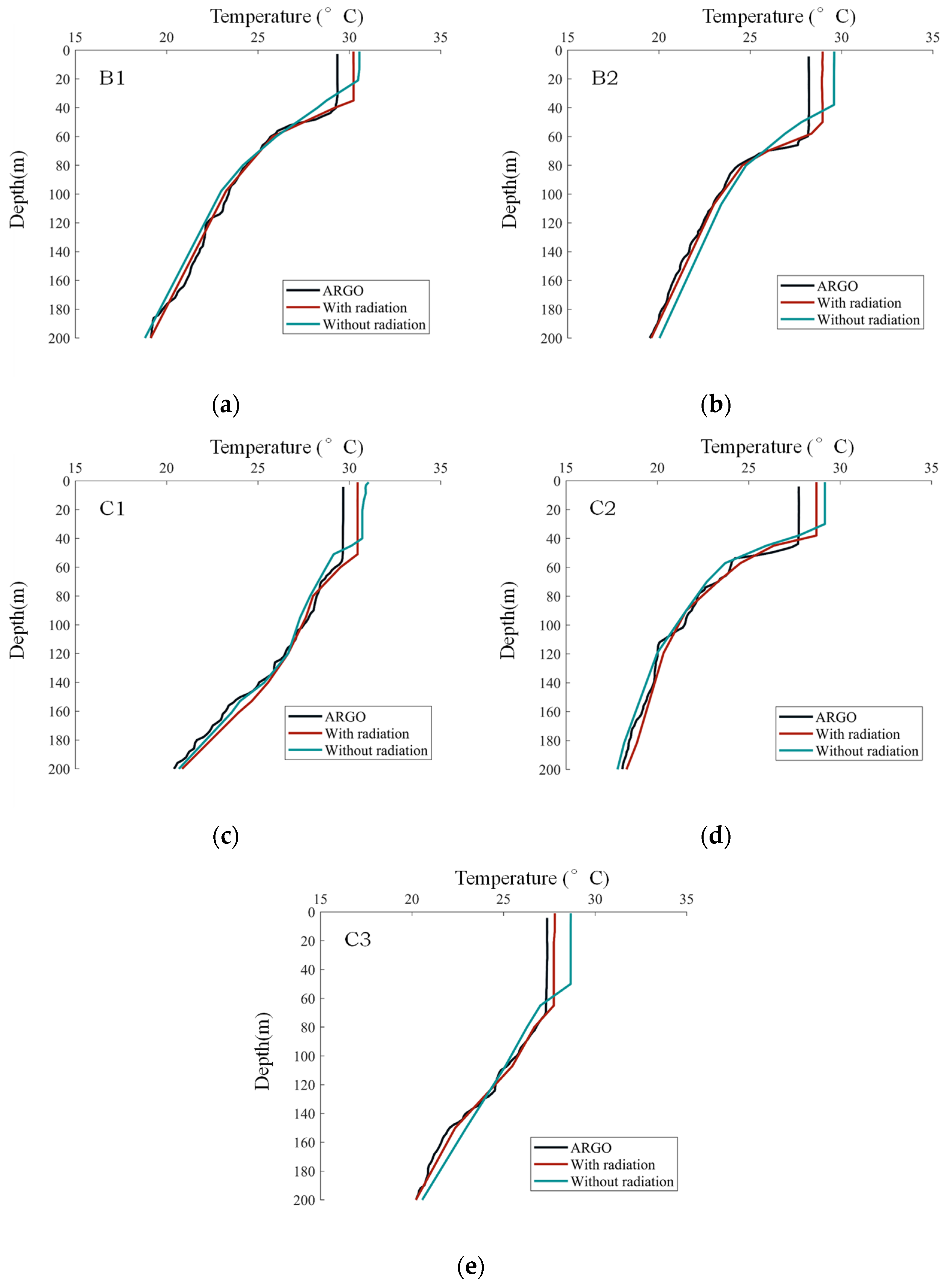
In the WNP, nine buoys at various latitudes and longitudes were chosen (Figure 1c). The buoys were compared to the simulation results with and without radiation stress (Figure 9). The temperature profile simulated with radiation stress was more similar to the temperature profile observed by the buoys. Based on the comparison of the vertical simulation results with and without radiation stress, the radiation stress first caused surface changes, the upwelling caused by the divergence of the upper water body indirectly affected the whole mixed layer. The reason is that radiation stress changes the sea surface current distribution as one of the wave-induced stress terms which directly affects the energy conservation equation further affecting the SST [24,43].
The vertical temperature profile of the southern region showed a thicker warm surface layer than that in the northern region in the WNP, which is consistent with the simulation results of D’Asaro [42]. In other words, the thermocline of WNP becomes shallower northward. This trend can be roughly indicated in Figure 9a–e. The influence depth of radiation stress varies with latitude in Figure 9a–e. From C1, C2, and B1, as the latitude gradually moves northward, the approximate depth of the influence ranges 56 m, 43 m, and 38 m, respectively. The temperature profiles in Figure 9 show that by taking the radiation stress into account, the upper boundary of the thermocline can be determined more accurately, the analysis of the thermocline characteristics can be improved with an RMSE of less than 1.63 °C and a COR of about 0.94.
3.5. Effect on Curreant Field
The dynamics during typhoons are complex. Previous works suggested that radiation stress, one of the wave-induced stress terms, changes the sea surface current distribution, which directly affects the energy conservation equation, further affecting the SST [24,43].
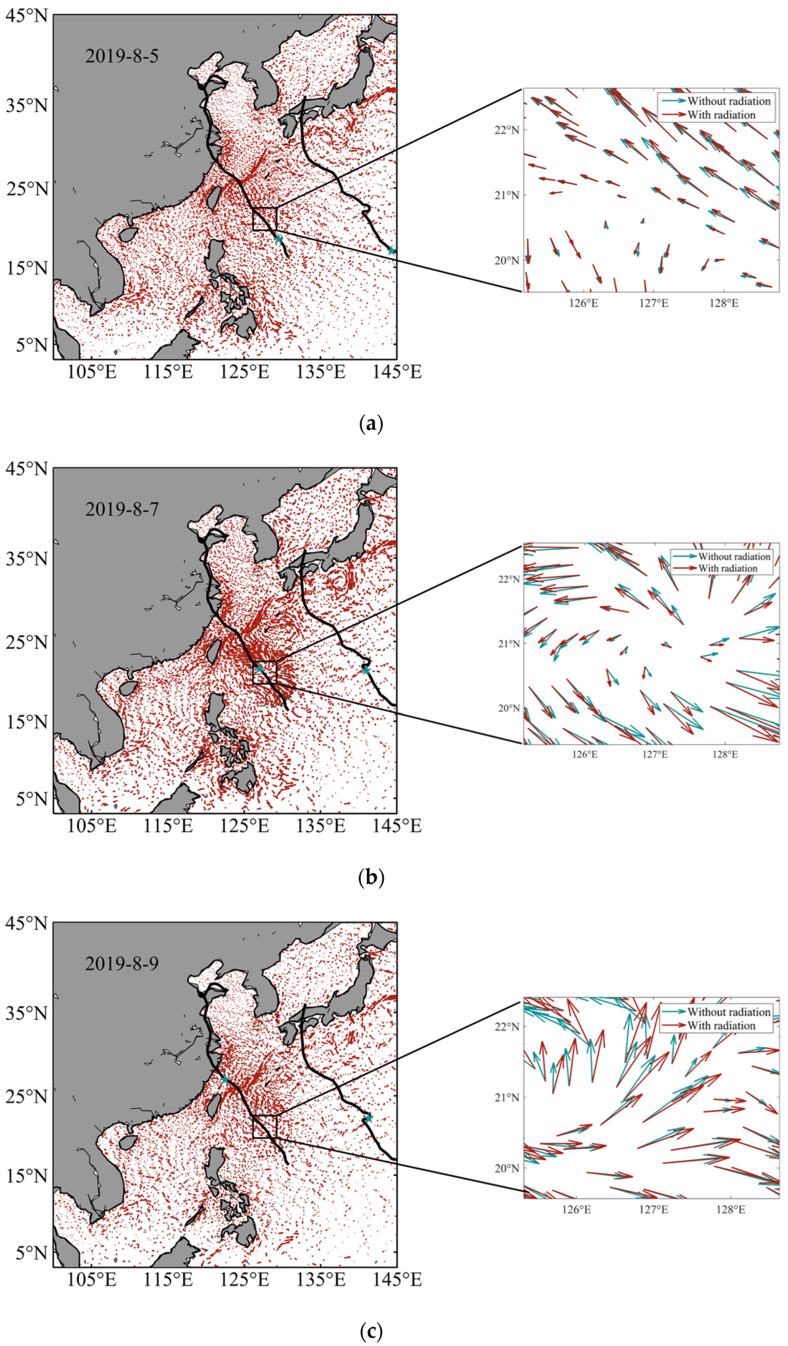
Figure 10 depicts the surface current field. During the simulation period, wave-induced radiation stress brings about surface current deviation to the right. For a more intuitive comparison, we plotted surface current vector diagrams with and without radiation stress in a single figure (Figure 10). In Figure 10, the total current field is shown on the left, with the zoomed area located along the typhoon path, and the enlarged view is shown on the right. Figure 10a–c depicts the current field with and without considering wave-induced radiation stress before, during, and after Typhoon L’s passage. Typhoon L did not pass through the zoomed area on 5 August, and the current direction of the surface current field shifted slightly to the right. Typhoon L passed through the zoomed area leading to the change of current field direction on 7 August. The majority of areas showed apparent rightward deviation, with a few left deviations in the direction of the typhoon. Typhoon L had already passed through the zoomed area on 9 August. There was an obvious deviation to the right on the side near the typhoon, and the deviation amplitude was even greater than when it passed through the area on 5 August. On the side far from the typhoon, the direction deflection was not obvious.
Furthermore, the deflection amplitude of the surface current field on 9 August was greater than that on 5 August, possibly due to the influence of Typhoon R on the right. On 9 August, the airflow of R entered the L wind field from the east through rotation, which strengthened the surface current and further changed the horizontal current field. It is suggested that wave radiation stress enhances the surface current and causes certain rightward deviation.
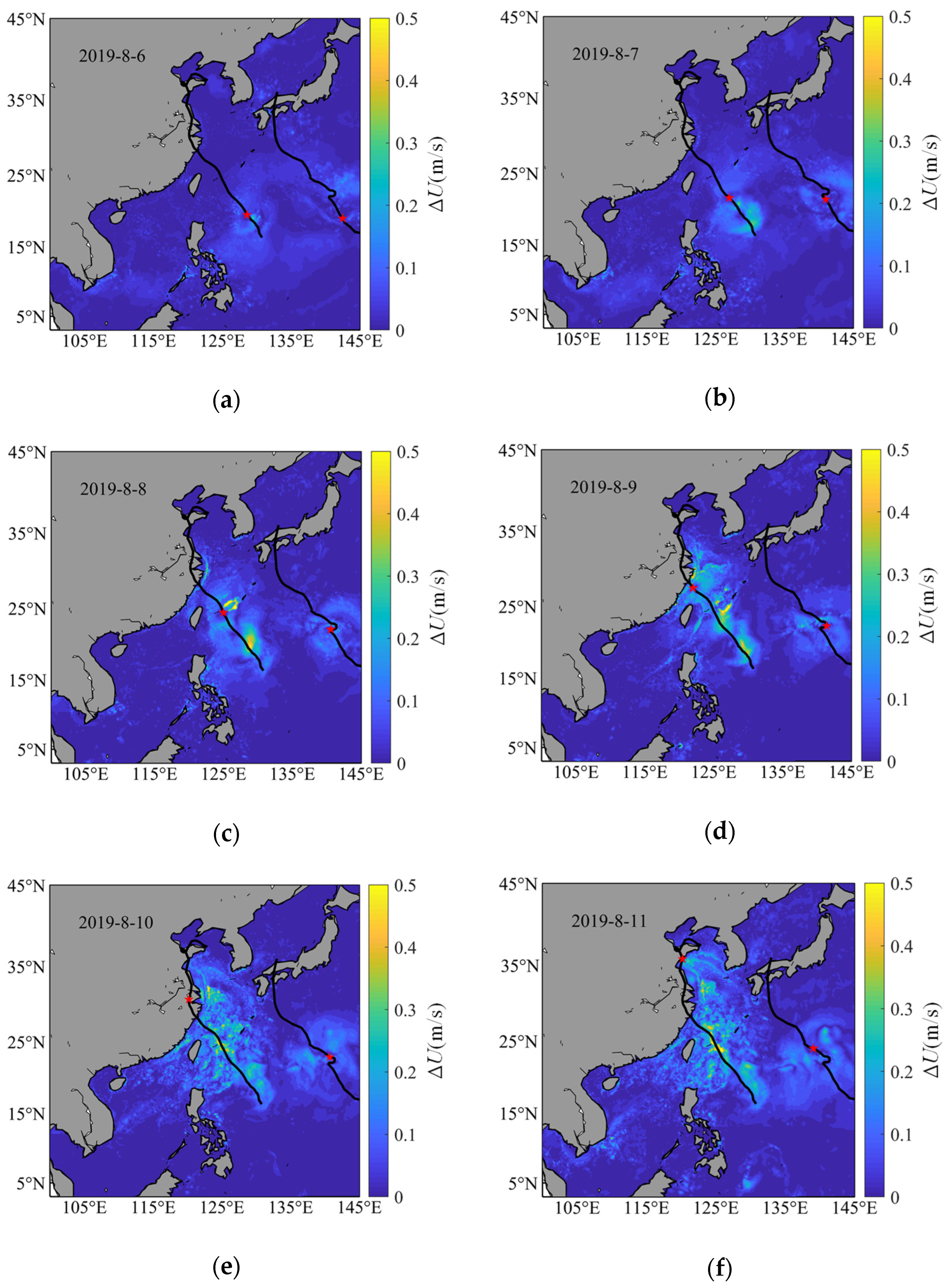
With a view to compare the influence of radiation stress on the surface current field during typhoons more intuitively, the surface current field simulated by FVCOM is subtracted from FVCOM-SWAVE. The surface current field exhibits a significant cyclonic structure under wave action (Figure 10). The change of the current field on the right side of the typhoon is greater than that on the left side (Figure 11). This shift in the surface current field also corresponds to the SWH distribution (Figure 2).
Typhoon waves began to make a difference in the current field on 6 August 2019. The surface current field showed a cyclonic change of around 0.25 m/s, with the change on the right side of the path being 0.1 m/s larger than the change on the left side (Figure 11a). In the early stages of typhoon development, it was thought to be primarily influenced by both waves and wind stress. The current field peaked at about 0.45 m/s as the intensity of L peaked on the night of 8 August, with another substantial current change area developing on the right side of the path likewise (Figure 11c).
Compared with L, the changes in the surface current field caused by R were not obvious. Some cyclonic changes began to appear on 7 August at about 0.14 m/s, with the current on the right side of the path changing more than the current on the left (Figure 11b). Subsequently, the changed area gradually grew, peaking at 0.21 m/s on 11 August (Figure 11f). Because of the comparatively slow velocity, the shift in the surface current field generated by R was not noticeable if compared to L. On 9 August, the airflow of R rotated to the L wind field from the east, which strengthened the surface current and further changed the horizontal current field (Figure 11d). As can be seen, the changes in the surface current field caused by radiation stress were continuous modifications.
4. Conclusions
The aim of this paper was to use FVCOM-SWAVE to investigate the upper-layer ocean temperature decrease in response to radiation stress. Previous studies [2,3,4,5,6] have considered sea surface cooling caused by typhoons. Here, we investigated the influence of wave-induced radiation stress on upper-layer ocean temperature (Including SST and mixed-layer temperature). This paper investigated not only the influence of radiation stress on the surface current field but also considers the influence of double typhoons.
Wave-induced radiation stress has an impact on ocean dynamics and the distribution of upper-ocean components. If the wave-induced radiation stress was taken into account, the bias in the SST data derived from the FVCOM-SWAVE simulation was reduced by around 1 °C compared to the FVCOM simulation. Meanwhile, the average mixed-layer temperature was verified by ARGO observations, with an RMSE of less than 1.63 °C and a COR of approximately 0.94. Therefore, we concluded that wave-induced radiation stress should be included in upper-layer ocean temperature simulations during typhoons because typhoon waves influence the mixing layer via radiation stress. The wave-induced radiation stress enhances the surface current and causes certain deviation to the right, causing the upper water diverges and upwelling increases, resulting in a decrease in SST.
The variations of the surface current field during typhoons were analyzed. If the surface current field with and without radiation stress is compared, it is discovered that wave radiation stress enhances the surface current and causes certain rightward deviations. Furthermore, the variation of the surface current field caused by radiation stress is obviously related to the distribution of SWH. The changes in the surface current field caused by radiation stress are continuous modifications and still exist after the typhoon passes, indicating a delayed response.
The wave-induced radiation stress affects the simulation of SST, reducing the SST simulation error. The results suggest that wave-induced radiation stress should be taken into account when simulating SST. Mixed-layer temperatures under typhoon conditions were also analyzed. Even though radiation stress initially only causes surface changes, upwelling caused by upper water body divergence indirectly affects the entire mixed layer. At the depths above the thermocline, the effect of radiation stress on the thermocline is more visible. If the influence of double typhoons is considered, the airflow of L rotates from the northwest toward R, limiting the development of SWH and reducing the cooling range.
As a result, this paper has been validated and should be recommended for predicting WNP sea conditions. In future research, we aim to investigate the Stokes drift effect using the same numerical model (FVCOM-SWAVE) under the condition of double typhoons and compare the simulation results of the Stokes drift spectrum parameterization scheme and several approximate parameterization schemes for SST.
Supplementary Materials
The following supporting information can be downloaded at: https://www.mdpi.com/article/10.3390/rs15092442/s1, Figure S1: The computational grid of the model domain, shading indicating water depth.
Author Contributions
Conceptualization, J.S.; methodology, Q.W. and J.S.; formal analysis, W.Z., J.S. and Q.W.; writing—original draft preparation, Q.W. and J.X.; writing—review and editing, H.W., J.X., K.H., W.X., J.L. and Q.W.; supervision, J.X., W.X. and J.S. All authors have read and agreed to the published version of the manuscript.
Funding
This research received no external funding.
Data Availability Statement
The typhoon best track dataset was obtained from the National Weather Service [44] (http://tcdata.typhoon.gov.cn/, accessed on 1 May 2023). The topographic data were available from NOAA National Centers (http://www.ngdc.noaa.gov/mgg/global/global.html, accessed on 1 May 2023). The wind data can be found in the ECMWF (https://www.ecmwf.int/, accessed on 1 May 2023). The daily averaged heat flux data were provided by the NCEP (https://downloads.psl.noaa.gov/Datasets/ncep.reanalysis/surface_gauss/, accessed on 1 May 2023). The initial temperature field and the salinity field were obtained from the HYCOM (https://www.hycom.org/, accessed on 1 May 2023). The Argo float profile data are available from the International ARGO Program and the national programs (http://www.argo.org.cn, accessed on 1 May 2023).
Acknowledgments
The authors thank the National Weather Service for providing the best track dataset of typhoons, NOAA National Centers for providing topographic data, ECMWF for providing the wind data, NCEP for providing the daily averaged heat flux data, and International Argo Program and the national programs for the Argo float profile data.
Conflicts of Interest
The authors declare no conflict of interest.
References
- Guan, S.D.; Li, S.Q.; Hou, Y.J.; Hu, P.; Liu, Z.; Feng, J.Q. Increasing threat of landfalling typhoons in the western North Pacific between 1974 and 2013. Int. J. Appl. Earth Obs. 2018, 68, 279–286. [Google Scholar] [CrossRef]
- Lin, I.I.; Liu, W.T.; Wu, C.C.; Wong, G.T.F.; Hu, C.; Chen, Z.; Liang, W.D.; Yang, Y.; Liu, K.K. New evidence for enhanced ocean primary production triggered by tropical cyclone. Geophys.Res. Lett. 2003, 30, 1718. [Google Scholar] [CrossRef]
- Sun, L.; Yang, Y.J.; Xian, T.; Lu, Z.M.; Fu, Y.F. Strong enhancement of chlorophyll a concentration by a weak typhoon. Mar. Ecol.Prog. Ser. 2010, 404, 39–50. [Google Scholar] [CrossRef]
- Price, J.F. Upper ocean response to a hurricane. J. Phys. Oceanogr. 1981, 11, 153–175. [Google Scholar] [CrossRef]
- D’Asaro, E.A.; Black, P.G.; Centurioni, L.R.; Chang, Y.T.; Chen, S.S.; Foster, R.C.; Graber, H.C.; Harr, P.; Hormann, V.; Lien, R.C.; et al. Impact of typhoons on the ocean in the Pacific. Bull. Amer. Meteor. Soc. 2014, 95, 1405–1418. [Google Scholar] [CrossRef]
- Price, J.F.; Sanford, T.B.; Forristall, G.Z. Forced stage response to a moving hurricane. J. Phys. Oceanogr. 1994, 24, 233–260. [Google Scholar] [CrossRef]
- D’Asaro, E.A. The ocean boundary layer below Hurricane Dennis. J. Phys. Oceanogr. 2003, 33, 561–579. [Google Scholar] [CrossRef]
- D’Asaro, E.A.; Sanford, T.B.; Niiler, P.P.; Terrill, E.J. Cold wake of hurricane Frances. Geophys. Res. Lett. 2007, 34, L15609. [Google Scholar] [CrossRef]
- Guan, S.D.; Zhao, W.; Sun, L.; Zhou, C.; Liu, Z.; Hong, X.; Zhang, Y.H.; Tian, J.W.; Hou, Y.J. Tropical cyclone-induced sea surface cooling over the Yellow Sea and Bohai Sea in the 2019 Pacific typhoon season. J. Marine Syst. 2021, 217, 103509. [Google Scholar] [CrossRef]
- Han, S.; Wang, M.; Peng, B. Response of Temperature to Successive Typhoons in the South China Sea. J. Mar. Sci. Eng. 2022, 10, 1157. [Google Scholar] [CrossRef]
- Jacob, S.D.; Shay, L.K.; Mariano, A.J.; Black, P.G. The 3D oceanic mixed layer response to Hurricane Gilbert. J. Phys. Oceanogr. 2000, 30, 1407–1429. [Google Scholar] [CrossRef]
- Huang, P.S.; Sanford, T.B.; Imberger, J. Heat and turbulent kinetic energy budgets for surface layer cooling induced by the passage of Hurricane Frances (2004). J. Geophys. Res. Oceans. 2009, 114, C12023. [Google Scholar] [CrossRef]
- Mei, W.; Pasquero, C. Spatial and temporal characterization of sea surface temperature response to tropical cyclones. J. Clim. 2013, 26, 3745–3765. [Google Scholar] [CrossRef]
- Kantha, I.H.; Clayson, C.A. An improved mixed layer model for geophysical applications. J. Geophys. Res. 1994, 99, 25235–25266. [Google Scholar] [CrossRef]
- Martin, P.J. Simulation of the mixed layer at OWS November and Papa with several models. J. Geophys. Res. 1985, 90, 581–597. [Google Scholar] [CrossRef]
- Kemp, P.H.; Simons, R.R. The interaction between waves and a turbulent current: Waves propagating with the current. J. Fluid Mech. 1982, 116, 73–89. [Google Scholar] [CrossRef]
- Mellor, G.L.; Donelan, M.A.; Oey, L.-Y. A Surface Wave Model for Coupling with Numerical Ocean Circulation Models. J. Atmos. Ocean Technol. 2008, 25, 1785–1807. [Google Scholar] [CrossRef]
- Longuet-Higgins, M.S.; Stewart, R.W. Radiation stresses in water waves: A physical discussion with applications. J. Deep-Sea Res. 1964, 11, 529–562. [Google Scholar] [CrossRef]
- James, I.D. Nonlinear waves in the nearshore region: Shoaling and set-up. Estuar. Coast. Mar. Sci. 1974, 2, 207–334. [Google Scholar] [CrossRef]
- Feddersen, F. Effect of wave directional spread on the radiation stress: Comparing theory and observations. Coast. Eng. 2004, 51, 473–481. [Google Scholar] [CrossRef]
- Zheng, Y.H.; Shen, Y.M.; Qiu, D.H. Calculation of wave radiation stress in combination with parabolic mild slope equation. China Ocean Eng. 2000, 14, 495–502. [Google Scholar]
- Li, L.; Xu, J.; Ren, Y.; Wang, X.H.; Xia, Y. Effects of wave-current interactions on sediment dynamics in Hangzhou Bay during Typhoon Mitag. Front. Earth Sci. 2023, 10, 88. [Google Scholar] [CrossRef]
- Dai, D.; Qiao, F.; Sulisz, W.; Han, L.; Babanin, A. An experiment on the nonbreaking surface-wave-induced vertical mixing. J. Phys. Oceanogr. 2010, 40, 2180–2188. [Google Scholar] [CrossRef]
- Sun, Z.; Shao, W.; Yu, W.; Li, J. A study of wave-induced effects on sea surface temperature simulations during typhoon events. J. Mar. Sci. Eng. 2021, 9, 622. [Google Scholar] [CrossRef]
- Qiao, F.; Yuan, Y.; Yang, Y.; Zheng, Q.; Xia, C.; Ma, J. Wave-induced mixing in the upper ocean: Distribution and application to a global ocean circulation model. Geophys. Res. Lett. 2004, 31, 622. [Google Scholar] [CrossRef]
- Sun, Y.; Perrie, W.; Toulany, B. Simulation of wave-current interactions under hurricane conditions using an unstructured-grid model: Impacts on ocean waves. J.Geophys.Res. 2018, 123, 3739–3760. [Google Scholar] [CrossRef]
- Han, G.; Ma, Z.; deYoung, B.; Foreman, M.; Chen, N. Simulation of three-dimensional circulation and hydrography over the Grand Banks of Newfoundland. Ocean. Model. 2011, 40, 199–210. [Google Scholar] [CrossRef]
- Rego, J.L.; Li, C. On the Receding of Storm Surge along Louisiana’s Low-Lying Coast. J. Coast Res. 2009, 2, 1045–1049. [Google Scholar]
- Chen, C.; Beardsley, R.C.; Cowles, G. An Unstructured Grid, Finite-Volume Community Ocean Model: FVCOM User Manual; Sea Grant College Program, Massachusetts Institute of Technology: Cambridge, MA, USA, 2011. [Google Scholar]
- Chen, C.S.; Beardsley, R.C.; Cowles, G. An unstructured grid, finite-volume coastal ocean model (FVCOM) system. Adv. Comput. Oceanogr. 2006, 19, 78–89. [Google Scholar] [CrossRef]
- Chen, C.; Huang, H.; Beardsley, R.C.; Liu, H.; Xu, Q.; Cowles, G. A finite volume numerical approach for coastal ocean circulation studies: Comparisons with finite difference models. J. Geophys. Res. 2007, 112, C03018. [Google Scholar] [CrossRef]
- Huang, H.; Chen, C.; Cowles, G.W.; Winant, C.D.; Beardsley, R.C.; Hedstrom, K.S.; Haidvogel, D.B. FVCOM validation experiments: Comparisons with ROMS for three idealized barotropic test problems. J. Phys. Oceanogr. 2008, 113, C07042. [Google Scholar] [CrossRef]
- Chen, C.; Liu, H.; Beardsley, R.C. An unstructured grid, finite-volume, three-dimensional, primitive equations ocean model: Application to coastal ocean and estuaries. J. Atmos. Ocean Technol. 2003, 20, 159–186. [Google Scholar] [CrossRef]
- Qi, J.; Chen, C.; Beardsley, R.C.; Perrie, W.; Cowles, G.W.; Lai, Z. An unstructured-grid finite-volume surface wave model (FVCOM-SWAVE): Implementation, validations and applications. Ocean Model. 2009, 28, 153–166. [Google Scholar] [CrossRef]
- Booij, N.; Ris, R.C.; Holthuijsen, L.H. A third generation wave model for coastal regions: 1. Model description and validation. J. Geophys. Res. 1999, 104, 7649–7666. [Google Scholar] [CrossRef]
- SWAN Group. SWAN User Manual-SWAN Cycle III Version 40.91, Chap. 4; Delft University of Technology: Delft, The Netherlands, 2012; pp. 55–56. [Google Scholar]
- Eldeberky, Y. Nonlinear Transformations of Wave Spectra in the Nearshore Zone. Ph.D. Thesis, Faculty of Civil Engineering, Delft University of Technology, Delft, The Netherlands, 1996; p. 203. [Google Scholar]
- Sorourian, S.; Huang, H.; Li, C.; Justic, D.; Payandeh, A.R. Wave dynamics near Barataria Bay tidal inlets during spring-summer time. Ocean Model. 2020, 147, 101553. [Google Scholar] [CrossRef]
- Wu, L.; Chen, C.; Guo, P.; Shi, M.; Qi, J.; Ge, J. A FVCOM-based unstructured grid wave, current, sediment transport model, I. Model description and validation. J. Ocean Univ. China 2011, 10, 1–8. [Google Scholar] [CrossRef]
- Zhang, Y.; Liu, Y.; Guan, S.; Wang, Q.; Zhao, W.; Tian, J. Sudden Track Turning of Typhoon Prapiroon (2012) Enhanced the Upper Ocean Response. Remote Sens. 2023, 15, 302. [Google Scholar] [CrossRef]
- Liu, J.; Shi, J.; Zhang, W. Numerical simulation of the wave-induced Stokes drift effect on sea surface temperature in the North Pacific. Oceanol. Hydrobiol. Stud. 2019, 48, 381–403. [Google Scholar] [CrossRef]
- D’Asaro, E.; Black, P.; Centurioni, L.; Harr, P.; Jayne, S.; Lin, I.; Lee, C.; Morzel, J.; Mrvaljevic, R.; Niiler, P.; et al. Typhoon-ocean interaction in the western North Pacific: Part 1. Oceanography 2011, 24, 24–31. [Google Scholar] [CrossRef]
- Hasselmann, K. Wave-driven inertial oscillations. Geophys. Astrophys. Fluid Dyn. 1970, 1, 463–502. [Google Scholar] [CrossRef]
- Ying, M.; Zhang, W.; Yu, H.; Lu, X.; Feng, J.; Fan, Y.; Zhu, Y.; Chen, D. An Overview of the China Meteorological Administration Tropical Cyclone Database. J. Atmos. Ocean. Technol. 2014, 31, 287–301. [Google Scholar] [CrossRef]
Figure 1.
Map of the study area in the western North Pacific (WNP): (a) with color indicating water depth; (b) the track of Jason-3 altimeter; (c) the red star indicates the locations of WNP Argo buoys; and (d) Typhoon tracks in the study area; Green and red lines are the moving tracks of Typhoon L and Typhoon R, respectively.

Figure 2.
Spatial distribution of significant wave height (SWH) when the typhoons passed through the WNP (a–f) (The black arrow shows wind direction, and the red star indicates the typhoon location).
Figure 2.
Spatial distribution of significant wave height (SWH) when the typhoons passed through the WNP (a–f) (The black arrow shows wind direction, and the red star indicates the typhoon location).

Figure 3.
Spatial distribution of surface velocity when the typhoons passed through the WNP (a–d) (the red star indicates the typhoon location).
Figure 3.
Spatial distribution of surface velocity when the typhoons passed through the WNP (a–d) (the red star indicates the typhoon location).

Figure 4.
Temperature differences when the typhoons passed through the WNP (a–f) (the red star indicates the typhoon location).
Figure 4.
Temperature differences when the typhoons passed through the WNP (a–f) (the red star indicates the typhoon location).

Figure 5.
Comparison of simulated SWH results and Jason-3 satellite data (a–d).

Figure 6.
Differences between sea surface temperature (SST) values simulated without the radiation stress and Sea Surface Temperature (OISST) data when the typhoons passed through the WNP (a–d) (the red star indicates the typhoon location).
Figure 6.
Differences between sea surface temperature (SST) values simulated without the radiation stress and Sea Surface Temperature (OISST) data when the typhoons passed through the WNP (a–d) (the red star indicates the typhoon location).

Figure 7.
Spatial distribution of SST difference due to radiation stress when the typhoons passed through the WNP (a–f) (the red star indicates the typhoon location).
Figure 7.
Spatial distribution of SST difference due to radiation stress when the typhoons passed through the WNP (a–f) (the red star indicates the typhoon location).

Figure 8.
Differences between SST values simulated with the radiation stress and OISST data when the typhoons passed through the WNP (a–d) (the red star indicates the typhoon location).
Figure 8.
Differences between SST values simulated with the radiation stress and OISST data when the typhoons passed through the WNP (a–d) (the red star indicates the typhoon location).

Figure 9.
Comparison of simulated and buoy-measured temperature profiles (a–e) (Following the buoy position in Figure 1c).
Figure 9.
Comparison of simulated and buoy-measured temperature profiles (a–e) (Following the buoy position in Figure 1c).

Figure 10.
Surface current vector field before, during, and after typhoons (a–c) (The green star indicates the typhoon’s location).
Figure 10.
Surface current vector field before, during, and after typhoons (a–c) (The green star indicates the typhoon’s location).

Figure 11.
Spatial distribution of surface current variation with and without radiation stress when the typhoons passed through the WNP (a–f) (the red star indicates the typhoon location).
Figure 11.
Spatial distribution of surface current variation with and without radiation stress when the typhoons passed through the WNP (a–f) (the red star indicates the typhoon location).


Table 1.
Comparison of simulated values and satellite data.
| Track | Satellite Peak (m) | Simulated Peak (m) | PE | MAE | RMSE (m) | COR |
|---|---|---|---|---|---|---|
| a | 2.738 | 2.358 | 0.380 | 0.363 | 0.328 | 0.843 |
| b | 6.348 | 6.306 | 0.004 | 0.218 | 0.534 | 0.969 |
| c | 6.916 | 5.790 | 1.126 | 0.212 | 0.499 | 0.974 |
| d | 3.870 | 3.314 | 0.556 | 0.184 | 0.238 | 0.986 |
Table 2.
Comparison of simulated subsurface temperature and buoy data.
| Buoy | With Radiation Stress | Without Radiation Stress | ||||||
|---|---|---|---|---|---|---|---|---|
| MAPE (°C) | COR | RMSE (°C) | SS | MAPE (°C) | COR | RMSE (°C) | SS | |
| A1 | 0.16 | 0.95 | 1.03 | 0.87 | 0.19 | 0.92 | 1.17 | 0.85 |
| A2 | 0.02 | 0.97 | 0.83 | 0.9 | 0.04 | 0.95 | 0.97 | 0.87 |
| B1 | 0.12 | 0.98 | 0.76 | 0.89 | 0.24 | 0.96 | 0.87 | 0.86 |
| B2 | 0.14 | 0.88 | 1.63 | 0.85 | 0.21 | 0.86 | 1.83 | 0.83 |
| C1 | 0.03 | 0.98 | 0.5 | 0.91 | 0.05 | 0.98 | 0.74 | 0.88 |
| C2 | 0.18 | 0.89 | 1.53 | 0.84 | 0.2 | 0.87 | 1.78 | 0.80 |
| C3 | 0.14 | 0.97 | 0.96 | 0.91 | 0.33 | 0.95 | 1.23 | 0.89 |
| D1 | 0.03 | 0.9 | 1.63 | 0.83 | 0.03 | 0.88 | 1.89 | 0.79 |
| E1 | 0.05 | 0.95 | 1.23 | 0.83 | 0.07 | 0.95 | 1.46 | 0.80 |
| Average | 0.94 | 1.12 | 0.87 | 0.15 | 0.92 | 1.33 | 0.84 | |
Disclaimer/Publisher’s Note: The statements, opinions and data contained in all publications are solely those of the individual author(s) and contributor(s) and not of MDPI and/or the editor(s). MDPI and/or the editor(s) disclaim responsibility for any injury to people or property resulting from any ideas, methods, instructions or products referred to in the content. |
© 2023 by the authors. Licensee MDPI, Basel, Switzerland. This article is an open access article distributed under the terms and conditions of the Creative Commons Attribution (CC BY) license (https://creativecommons.org/licenses/by/4.0/).
Share and Cite
MDPI and ACS Style
Wang, Q.; Shi, J.; Xia, J.; Han, K.; Xiao, W.; Zhang, W.; Wang, H.; Lv, J. Influence of Wave-Induced Radiation Stress on Upper-Layer Ocean Temperature during Typhoons. Remote Sens. 2023, 15, 2442. https://doi.org/10.3390/rs15092442
AMA Style
Wang Q, Shi J, Xia J, Han K, Xiao W, Zhang W, Wang H, Lv J. Influence of Wave-Induced Radiation Stress on Upper-Layer Ocean Temperature during Typhoons. Remote Sensing. 2023; 15(9):2442. https://doi.org/10.3390/rs15092442
Chicago/Turabian StyleWang, Qianhui, Jian Shi, Jingmin Xia, Kaifeng Han, Wenbin Xiao, Wenjing Zhang, Haodi Wang, and Jialei Lv. 2023. "Influence of Wave-Induced Radiation Stress on Upper-Layer Ocean Temperature during Typhoons" Remote Sensing 15, no. 9: 2442. https://doi.org/10.3390/rs15092442
Note that from the first issue of 2016, this journal uses article numbers instead of page numbers. See further details here.